Báo cáo hóa học: " Novel Multistatic Adaptive Microwave Imaging Methods for Early Breast Cancer Detection" potx
Bạn đang xem bản rút gọn của tài liệu. Xem và tải ngay bản đầy đủ của tài liệu tại đây (2.4 MB, 13 trang )
Hindawi Publishing Corporation
EURASIP Journal on Applied Signal Processing
Volume 2006, Article ID 91961, Pages 1–13
DOI 10.1155/ASP/2006/91961
Novel Multistatic Adaptive Microwave Imaging Methods
for Early Breast Cancer Detection
Yao Xie,
1
Bin Guo,
1
Jian Li,
1
and Petre Stoica
2
1
Department of Electrical and Computer Engineering, University of Florida, P.O. Box 116200, Gainesville, FL 32611-6200, USA
2
Systems and Control Division, Department of Information Technology, Uppsala University, P.O. Box 337,
75105 Uppsala, Sweden
Received 19 October 2005; Accepted 21 December 2005
Multistatic adaptive microwave imaging (MAMI) methods are presented and compared for early breast cancer detection. Due to
the significant contrast between the dielectric properties of normal and malignant breast tissues, developing microwave imaging
techniques for early breast cancer detection has attracted much interest lately. MAMI is one of the microwave imaging modalities
and employs multiple antennas that take tur ns to transmit ultra-wideband (UWB) pulses while all antennas are used to receive
the reflected signals. MAMI can be considered as a special case of the multi-input multi-output (MIMO) radar with the multiple
transmitted waveforms being either UWB pulses or zeros. Since the UWB pulses transmitted by different antennas are displaced
in time, the multiple transmitted waveforms are orthogonal to each other. The challenge to microwave imaging is to improve
resolution and suppress strong interferences caused by the breast skin, nipple, and so forth. The MAMI methods we investigate
herein utilize the data-adaptive robust Capon beamformer (RCB) to achieve high resolution and interference suppression. We will
demonstrate the effectiveness of our proposed methods for breast cancer detection via numerical examples with data simulated
using the finite-difference time-domain method based on a 3D realistic breast model.
Copyright © 2006 Hindawi Publishing Corporation. All rights reserved.
1. INTRODUCTION
Breast cancer takes a tremendous toll on our society. One in
eight women in the US will get breast cancer in h er lifetime
[1]. Each year more than 200 000 new cases of invasive breast
cancer are diagnosed and more than 40 000 women die from
the disease in the US alone [1]. Early diagnosis is currently
the best hope of surviving breast cancer.
Currently, X-ray mammography is the standard routine
breast cancer screening tool. However, the effectiveness of X-
ray mammography has been questioned by certain sources
in recent years and is somewhat currently under debate due
to its inherent limitations in resolving both low- and high-
contrast lesions and masses in radiologically dense glandu-
lar breast tissues. Breast tissues of younger women typically
present a higher ratio of dense to fatty tissues, limiting the
effectiveness of X-ray mammography. Hence mammogra-
phy presents its major limitation in the sector of the popu-
lation of highest public health interest and criticality. Some
techniques such as magnetic resonance imaging (MRI) and
Positron emission tomography (PET) have led to an increase
in the identification of small abnormalities in the human
breast, but the widespread use of MRI and PET for routine
breast cancer screening is unlikely due to their high costs.
Ultra-wideband (UWB) confocal microwave imaging
(CMI) is one of the most promising and attractive new
screening technologies currently under development: it is
nonionizing (safe), noninvasive (comfortable), sensitive (to
tumors), specific (to cancers), and low-cost [2]. Its physical
basis lies in the significant contrast in the dielectric proper-
ties between normal and malignant breast tissues [3–7]. In
CMI, UWB pulses are transmitted f rom antennas at differ-
ent locations near the breast surface and the backscattered
responses from the breast are recorded, from which the im-
age of the backscattered energy distribution is reconstructed
coherently.
The data acquisition approaches and the associated signal
processing methods affect the CMI imaging quality. There
are three major data acquisition schemes: monostatic [8],
bistatic [9, 10], and multistatic [11]. For monostatic CMI,
the transmitter is also used as a receiver and is moved across
the breast to form a synthetic aperture. For bistatic CMI,
one transmitting and one receiving antenna are used as a
pair and moved across the breast to form a synthetic aper-
ture. For multistatic CMI, a real aperture array (see Figure 1)
is used for data collection. Each antenna in the array takes
turns to transmit a probing pulse, and all antennas (in some
cases, all except the transmitting antenna) are used to receive
2 EURASIP Journal on Applied Signal Processing
Tumor
Antenna array
x
y
z
Figure 1: Antenna array configuration.
the backscattered signals. Multistatic CMI can be consid-
ered as a special case of the wideband multi-input multi-
output (MIMO) radar [12–14] with the multiple transmit-
ted waveforms being either UWB pulses or zeros. Since the
UWB pulses transmitted by different antennas are displaced
in time, the multiple transmitted waveforms are orthogonal
to each other. The monostatic and bistatic schemes exploit
the transmitter spatial diversity, and the multistatic scheme
takes advantage of the transmitter-and-receiver spatial diver-
sity. The multistatic approach can give better imaging results
than its mono- or bistatic counterparts when the synthetic
aperture formed by the latter two approaches is similar to
the real aperture array used by the former. An intuitive ex-
planation would be that the multistatic approach utilizes the
receiver diversity as well, by simultaneously recording mul-
tiple received signals that propagate via different routes and
hence accrues more information about the tumor.
The challenge to CMI imaging is to devise signal pro-
cessing algorithms to improve resolution and suppress strong
interferences caused by the breast skin, nipple, and so
forth. Signal processing algorithms can be classified as data-
dependent (data-adaptive) and data-independent methods.
For mono- and bistatic ultra-wideband CMI, the simple
data-independent delay-and-sum (DAS) [8, 11], the data-
independent microwave imaging space-time (MIST) beam-
forming [15], the data-adaptive robust Capon beamforming
(RCB) [9, 10], as well as the data-adaptive amplitude and
phase estimation (APES) [9, 10] methods have been con-
sidered for image formation. For multistatic ultra-wideband
CMI, the DAS- [11]andRCB-basedadaptive[16] meth-
ods have been considered. The data-adaptive methods can
have better resolution and much better interference suppres-
sion capability and can significantly outperform their data-
independent counterparts.
In this paper, we consider multistatic adaptive microwave
imaging (MAMI) methods to form images of the backscat-
tered energy for early breast cancer detection. For a location
of interest (or focal point) r within the breast, the complete
recorded m ultistatic data can be represented by a cube, as
shown in Figure 2.In[16], we proposed a MAMI approach,
iM
Transm itte r
index
t
0
N − 1
Time
index
Receiver-
index slicing
MAMI-1
MAMI-2
Receiver
index
M
Figure 2: Multistatic CMI data cube model. In Stage I, MAMI-1
slices the data cube for each time index, whereas MAMI-2 slices the
data cube for each transmitter index. Then RCB is applied to each
data slice to obtain multiple waveform estimates.
referred to MAMI-1 herein, which is a two-stage time-
domain signal processing algorithm for multistatic CMI. In
Stage I, MAMI-1 slices the data cube corresponding to each
time index, and processes the data slice by the robust Capon
beamformer (RCB) [17–19] to obtain backscattered wave-
form estimates at each time instant. Based on these estimates,
in Stage II a scalar waveform is retrieved via RCB, the en-
ergy of which is used as an estimate of the backscattered en-
ergy for the focal point. MAMI-1 has been shown to have
better perfor mance than other existing methods. An alterna-
tive way of slicing the data cube in Stage I before applying
RCB is to select a slice corresponding to each transmitting
antenna index (see Figure 2). The so-obtained approach is
referred to as MAMI-2 herein. We will show that MAMI-
2 tends to yield better images than MAMI-1 for high input
signal-to-interference-noise ratio (SINR), but worse images
at low SINR. We will also show that combining MAMI-1 and
MAMI-2 yields good performance in all cases of SINR. We
refer to the combined method as MAMI-C herein.
We will demonstrate the performance of the MAMI
methods using data simulated with the finite difference time
domain (FDTD) method. The simulated breast models con-
sidered in the literature include a two-dimensional (2D)
model based on a breast MRI scan [8, 15], simple three-
dimensional (3D) and planar models [20], and the more re-
alistic 3D model [9, 10, 21]. Our simulations are based on
the 3D hemispherical breast model. The tumor response for
the realistic 3D model is much smaller than that for the 2D
(or 3D cylindrical) model due to tumor being assumed in-
finitely long in the latter model. The MAMI methods can de-
tect tumors as small as 4 mm in diameter based on the realis-
tic 3D model. Based on 2D models, the MAMI methods can
detect tumors as small as 1.5 mm in diameter. We have only
Yao Xie et al. 3
included the realistic 3D-model-based examples herein since
the conclusions drawn from 2D based models are similar.
The following notation will be used: (
·)
T
denotes the
transpose, R
m×n
stands for the Euclidean space of dimen-
sion m
× n, B 0 means that B is positive semidefinite, bold
lowercase symbols represent vectors, and bold capital letters
represent matrices.
2. DATA MODEL
We consider a multistatic imaging system, where K antennas
are arranged on a hemisphere relatively close to the breast
skin, at know n locations. The configuration of the array is
shown in Figure 1. The antennas are arranged on P layers
with Q antennas per layer, where K
= PQ. Each antenna
takes turns to transmit an UWB probing pulse while all of
the antennas are used to record the backscattered signals. Let
x
i, j
(t), i = 1, , K, j = 1, , K, t = 0, , N − 1, denote the
backscattered signal generated by the probing pulse sent by
the ith transmitting antenna and received by the jth receiving
antenna, where t denotes the time sample. The 3
× 1vectorr
denotes the focal point (i.e., an imaging location within the
breast). In our algorithms, the location r is varied to cover all
grid points of the breast model.
Our goal is to form a 3D image of the backscattered en-
ergy E(r) on a grid of points within the breast, with the scope
of detecting the tumor. The backscattered energy is estimated
from the complete received data
{x
i, j
(t)} for each location r
of interest.
Before image f ormation, we preprocess the received sig-
nals
{x
i, j
(t)} to remove, as much as possible, backscat-
tered signals other than the tumor response, to align all the
recorded signals from r by time-shifting, and to compensate
for the propagation loss of the signal amplitude. (See [16]for
details.) The preprocessed signals y
i, j
(t) obtained from x
i, j
(t)
can be described as
y
i, j
(t) = s
i, j
(t)+e
i, j
(t), i, j = 1, , K, t = 0, , N − 1,
(1)
where s
i, j
(t) represents the tumor response and e
i, j
(t)repre-
sents the residual term. The residual term e
i, j
(t) includes the
thermal noise and the interference due to undesired reflec-
tions from the breast skin, nipple, and so forth. To cast (1)in
a form suitable for the application of RCB [17], we approxi-
mate the data model (1) by making different assumptions. In
the follow ing we use t (t
= 0, , N − 1) to denote a generic
given time index, and i (i
= 1, , K)todenoteageneric
given transmitter index.
MAMI-1 approximates the data model (1)as
y
i
(t) = a(t)s
i
(t)+e
i
(t), (2)
where y
i
(t) = [y
i,1
(t), , y
i,K
(t)]
T
and e
i
(t) = [e
i,1
(t), ,
e
i,K
(t)]
T
. The scalar s
i
(t) denotes the backscattered signal
(from the focal point at location r) corresponding to the
probing signal from the ith transmitting antenna. The vector
a(t)in(2) is referred to as the array steering vector. Note that
a(t) is approximately equal to 1
K×1
since al l the signals have
been aligned temporally and their attenuations compensated
for in the preprocessing step.
There are three assumptions made to write the model in
(2). First, the steering vector is assumed to vary with t,but
be nearly constant with respect to i (the index of the trans-
mitting antenna). Second, we assume that the backscattered
signal waveform depends only on i but not on j (the index of
the receiving antenna). The truth, however, is that the steer-
ing vector is not exactly known and it changes slightly with
both t and i due to array calibration errors and other factors.
The signal waveform can also vary slightly with both i and
j, due to the (relatively insignificant) frequency-dependent
lossy medium within the breast. The two aforementioned
assumptions simplify the problem slightly. They cause little
performance degradations when used with our robust adap-
tive algorithms. Third, we assume that the residual term is
uncorrelated with the signal.
MAMI-2 approximates the data model (1)differently as
follows:
y
i
(t) = a
i
s
i
(t)+e
i
(t), (3)
where a
i
denotes the steering vector, which is again approxi-
mately 1
K×1
. The second and third assumptions used to ob-
tain (2) are also made to obtain (3). However, MAMI-2 as-
sumes that the steering vector varies with i, but is constant
with respect to t.
In practice, the steering vectors a(t)anda
i
may be im-
precise, in the sense that their elements may differ slightly
from 1. This uncertainty in the steering vector motivates us
to consider using RCB for waveform estimation. Because the
steering vectors in (2)and(3) are both approximately 1
K×1
,
we assume that the true steering vector a(t)ora
i
lies in uncer-
tainty spheres, the centers of which are the assumed steering
vector
¯
a
= 1
K×1
. (For the more general case of ellipsoidal un-
certainty sets, see [19] and the references therein.) The only
knowledge we assume about a(t)anda
i
is, respectively, that
a(t) −
¯
a
2
≤
1
,
a
i
−
¯
a
2
≤
2
,
(4)
where
1
and
2
are used to describe the amount of uncer-
tainty in a(t)anda
i
,respectively.
The choice of the uncertaint y size parameters,
1
and
2
,
as well as of their counterparts in Stage II of MAMI-1 and
MAMI-2 (see below), is determined by several factors such
as the sample size N and the array calibration errors [17, 18].
First, they should be made as small as possible. Otherwise the
ability of RCB to suppress an interference that is close to the
signal of interest will be lost. Second, The smaller the N or
the larger the steering vector errors, the larger should they
be chosen. T hird, to avoid t rivial solution to the optimiza-
tion problem of RCB, they should be less than the square of
4 EURASIP Journal on Applied Signal Processing
the norm of the assumed steering vector [17, 18]. Such qual-
itative guidelines are usually sufficient for the choice of the
uncertainty size parameters, since the performance of RCB
does not depend very critically on them (as long as they take
on “reasonable values”) [19]. In our numerical examples, we
choose certain reasonable initial values for them and then
make some adjustments empirically based on imaging quali-
ties (i.e., making them smaller when the current resulted im-
ages have low resolution or lots of clutter, or making them
larger when the target in the current resulted images appears
to be suppressed too).
3. MAMI-1 AND MAMI-2
In Stage I, both MAMI-1 and MAMI-2 obtain K signal wave-
form estimates via RCB. In Stage I of MAMI-2, for the ith
probing pulse, the true steering vector a
i
can be estimated
via the covariance fitting approach of RCB:
max
σ
2
i
,a
i
σ
2
i
subject to
R
Y
i
− σ
2
i
a
i
a
T
i
0,
a
i
−
¯
a
2
≤
2
,
(5)
where σ
2
i
is the power of the signal of interest, and
R
Y
i
=
1
N
Y
i
Y
T
i
(6)
is the sample covariance matrix with
Y
i
=
y
i
(0), y
i
(1), , y
i
(N − 1)
, Y
i
∈ R
K×N
. (7)
By using the Lagrange multiplier method, the solution to this
optimization problem is given by [17]
a
i
=
¯
a
−
I + ν
R
Y
i
−1
¯
a,(8)
where ν
≥ 0 is the corresponding Lagrange multiplier that
can be solved efficiently from the following equation (e.g.,
using the Newton method):
I + ν
R
Y
i
−1
¯
a
2
= ,(9)
since the left-hand side of (9) is monotonically decreasing in
ν (see [17] for more details). After determining the multiplier
ν,
a
i
is determined by (8). To eliminate a scaling ambiguity
(see [17]), we scale
a
i
to make a
i
2
= M. Then we can apply
the following weight vector to the received signals (see [17]
for details):
w
2,i
=
a
i
K
1/2
·
R
Y
i
+(1/ν)I
−1
¯
a
¯
a
T
R
Y
i
+(1/ν)I
−1
R
Y
i
R
Y
i
+(1/ν)I
−1
¯
a
(10)
to obtain the corresponding signal waveform estimate. Note
that (10) has a diagonal loading form, which can be used
even when the sample covariance matrix is rank-deficient.
The beamformer output can be written as the vector
s
i
=
w
T
2,i
Y
i
T
, s
i
∈ R
N×1
, (11)
which is the waveform estimate of the backscattered signal
(from the fixed location r) for the ith probing signal. Repeat-
ing the above process for i
= 1 through i = K,weobtain
the complete set of K waveform estimates
S
2
= [s
1
, ,s
K
]
T
,
S
2
∈ R
K×N
.
Similarly, in Stage I of MAMI-1, we obtain a set of wave-
form estimates
S
1
= [s(0), ,s(N − 1)],
S
1
∈ R
K×N
(see
[16] for details).
Note that Stage I of both MAMI-1 and MAMI-2 yields
K waveform estimates of the backscattered signals (one
for each transmitting antenna). Let
{s
1
(t)}
t=0, ,N −1
,and
{s
2
(t)}
t=0, ,N −1
denote the columns of the matrices
S
1
and
S
2
, respectively. Since all probing signals have the same wave-
form, we assume that the true backscattered signal wave-
forms are (nearly) identical. This means that, for example,
for MAMI-2, the elements of the vector
s
2
(t) are all approx-
imately equal to an unknown (scalar) signal s(t). So in Stage
II, we can employ RCB to recover a scalar waveform
s(t)
from
{s
1
(t)} or {s
2
(t)} (see [16] for more details on Stage
II of MAMI-1; Stage II of MAMI-2 is similar). Finally, the
backscattered energy E(r)iscomputedas
E(r)
=
N−1
t=0
s
2
(t). (12)
It is well known that the errors in sample covariance ma-
trices (e.g., the
R
Y
i
above) and the steering vectors cause per-
formance degradations in adaptive beamforming [22, 23].
Note that, on one hand, MAMI-2 uses more snapshots
(namely, N) than MAMI-1 (namely, K) to estimate the sam-
ple covariance matrix. Therefore, the sample covariance ma-
trix of MAMI-2 is more precise than that of MAMI-1. On
the other hand, MAMI-1 employs RCB N times, whereas
MAMI-2 uses RCB K times (recall that N>K), so there
is more “room” for robustness in MAMI-1 than in MAMI-2,
which means that MAMI-1 should be more robust to steer-
ing vector errors. In summary, MAMI-2 uses a more pre-
cise sample covariance matrix, whereas MAMI-1 is more ro-
bust against steering vector mismatch. Therefore, according
to what was said above, at high input SINR (when the sample
covariancematrixerrorsaremoreimportant)wecanexpect
MAMI-2 to perform better than MAMI-1, and vice versa at
low input SINR (when the errors in the steering vector are
critical).
4. MAMI-C
The previous intuitive discussions on MAMI-1 and MAMI-2
and the numerical examples presented later on imply that
Yao Xie et al. 5
MAMI-2 has better performance at high SINR, while MAMI-
1 usually outperforms MAMI-2 at low SINR. This fact mo-
tivates us to consider combining MAMI-1 and MAMI-2 to
achieve good performance in all cases of SINR. In the com-
bined method, which is referred to as MAMI-C, we use
the two sets of K waveform estimates yielded by Stage I of
MAMI-1 and Stage I of MAMI-2 simultaneously in Stage II
(note that MAMI-1 and MAMI-2 have a similar Stage II). In
this way the combined method increases the number of “fic-
titious” ar ray elements from K to 2K.
The combined set of estimated waveforms is denoted by
S
C
= [
S
T
1
S
T
2
]
T
,
S
C
∈ R
2K×N
, where the subscript (·)
C
stands
for MAMI-C. Let the 2K
×1vectors{s(t)}
t=0, ,N −1
denote the
columns of
S
C
. Stage II of MAMI-C consists of recovering a
scalar waveform from
{s(t)}.
The vector
s(t) is treated as a snapshot from a 2K-
element (fictitious) “array”:
s(t) = a
C
s(t)+e
C
(t), t = 0, , N − 1, (13)
where a
C
is assumed to belong to an uncertainty set centered
at
a = 1
2K×1
,ande
C
(t) represents the estimation error. Us-
ing RCB, we estimate a
C
and then obtain the adaptive weight
vector via an expression similar to (10):
w
C
=
a
C
K
1/2
·
R
C
+(1/μ)I
−1
a
a
T
R
C
+(1/μ)I
−1
R
C
R
C
+(1/μ)I
−1
a
,
(14)
where μ is the corresponding Lag range multiplier (see [17]
for more details), and
R
C
is the following sample covariance
matrix:
R
C
=
1
N
N−1
t=0
s(t)s
T
(t). (15)
The beamformer output gives an estimate of the signal of
interest:
s(t) = w
T
C
s(t). (16)
Finally, the backscattered energy at location r is computed
using (12).
Remark 1. It is natural to come up with a third way of slic-
ing the data cube in Stage I before applying RCB: to select
a slice corresponding to each receiving antenna index (see
Figure 2). Our numerical examples show that the perfor-
mance of this method is similar to that of MAMI-2. More-
over, we can use the waveform estimates from this approach
together with those estimated in Stage I of MAMI-1 and
Stage I of MAMI-2 to estimate a scalar waveform. However,
numerical examples show that such a combination provides
no significant improvement over MAMI-C, but the compu-
tational complexities increase due to the increased data di-
mension in Stage II. Therefore, we will not consider this op-
tion any further hereafter.
5. NUMERICAL EXAMPLES
We consider a 3D breast model as in [16]inournumeri-
cal examples. The model includes randomly distr ibuted fatty
breast tissue, glandular tissue, 2 mm-thick breast skin, as well
as the nipple and chest wall. To reduce the reflections from
the breast skin, the breast model is immersed in a lossless
liquid with permittivity similar to that of the breast fatty tis-
sue [24]. The breast model is a hemisphere with 10 cm in
diameter. A tumor that is 6 mm (or 4 mm) in diameter is lo-
cated 2.7 cm under the skin (at x
= 70 mm, y = 90 mm,
z
= 60 mm). Two cross-sections of the 3D model are shown
in Figure 3.
We assume that the dielectric properties (per mittivity
and conductivity) of the breast tissues are Gaussian random
variables with a mean equal to their nominal values and a
variance equal to 0.1 times their mean values. This variation
represents an upper bound on reported breast tissue variabil-
ities [4, 5]. The nominal values are chosen to be the typical
values reported in the literature [3–7], as shown in Table 1 .
Since UWB pulses are used as probing signals, the dispersive
properties of the fatty breast tissue and those of the tumor are
also considered in the model. The frequency dependencies
of the permittivity ε(ω) and conductivity σ(ω)aremodelled
according to a single-pole Debye model [8]. The randomly
distributed breast tissues with variable dielectric properties
represent the physical nonhomogeneity of the human breast.
As shown in Figure 1 , the antenna array consists of K
=
72 elements that are arranged on a hemisphere, which is 1 cm
away from the breast skin, on P
= 6 layers in the z-axis di-
mension. The layers of antennas are arranged along the z-axis
between 5.0 cm and 7.5 cm, with 0.5 cm spacing. Within each
layer, Q
= 12 antennas are placed on a cross-sectional circle
with uniform spacing. The UWB signal used is a Gaussian
pulse given by
G(t)
= exp
−
t − τ
0
τ
2
, (17)
where τ
0
= 25 μs, τ = 10 μs, and the pulse width is roughly
120 ps. Each antenna of the array takes turns to transmit the
Gaussian probing pulse, and all 72 antennas are used to re-
ceive the backscattered signals.
FDTD [25, 26] is used to obtain the simulated data. The
grid cell size used is 1 mm
× 1mm× 1 mm and the time step
is 1.667 ps. The model is terminated according to perfectly
matched layer absorbing boundary conditions [27]. The Z-
transform [28] is used to implement the FDTD method
whenever materials with frequency-dependent properties are
6 EURASIP Journal on Applied Signal Processing
20 40 60 80 100 120 140 160 180
x (mm)
Model: x
− y plane at z = 6cm
20
40
60
80
100
120
140
160
180
y (mm)
Glandular
tissue
Fat tissue
Tumor
Skin
Immersion
liquid
(a)
20 40 60 80 100 120 140 160 180
x (mm)
Model: x
− z plane at y = 9cm
20
40
60
80
100
120
z (mm)
Glandular
tissue
Fat tissue
Tumor
Skin
Immersion
liquid
Chest wall
(b)
Figure 3: Cross-sections of a 3D hemispherical breast model at (a) z = 60 mm and (b) y = 90 mm.
involved. Finally, the time window in the preprocessing step
consists of 150 samples, which means that N
= 150 for each
of the preprocessed signals.
The performance comparisons of MAMI-1 with other
existing methods can be found in [16]. In the following,
we focus on comparing MAMI-1 with the other two MAMI
methods.
In the follow ing examples, we add white Gaussian noise
with zero-mean and different variance values σ
2
0
to the re-
ceived signals. We define SNR (signal-to-noise ratio) as
SNR
= 10 log
10
×
1/K
2
K
i=1
K
j=1
(1/N)
N−1
t=0
ˇ
x
2
i, j
(t)
σ
2
0
dB,
(18)
and SINR as
SINR
= 10 log
10
×
1/K
2
K
i
=1
K
j
=1
(1/N)
N−1
t
=0
ˇ
x
2
i, j
(t)
1/K
2
K
i=1
K
j=1
(1/N)
N−1
t=0
ˇ
I
2
i, j
(t)
+σ
2
0
dB.
(19)
The
ˇ
x
i, j
(t)in(19) is the received signal due to the tumor only,
and
ˇ
I
i, j
(t) is due to the interference from breast skin, nipple,
and so forth (without tumor response), both of which are
not available in practice. To compute SNR and SINR, we per-
formed the simulation twice, with and without the tumor, re-
garded the second set of received signals as interference only,
Table 1: Nominal dielectric properties of breast tissues.
Tissues
Dielectric properties
Permittivity (F/m) Conductivity (S/m)
Immersion liquid 90
Chest wall
50 7
Skin
36 4
Fatty breast tissue
90.4
Nipple
45 5
Glandular tissue
11–15 0.4–0.5
Tumor
50 4
and used the difference between the two sets of received sig-
nals to approximate
ˇ
x
i, j
(t). All the images are displayed on
a logarithmic scale with a dynamic range of 40 dB (note that
here the dynamic range used is larger than the 20 dB dynamic
range in [16]).
Figures 4 and 5 show the CMI images of a 6 mm-diameter
tumor, at low and high thermal noise levels, respectively.
At the low noise level (SNR
= 12.1 dB, SINR =−1.4dB),
the images produced by MAMI-2 have much more focused
tumor responses than those of MAMI-1. The images of
MAMI-C have similar qualities to those of MAMI-2. In
Figure 5, at the high noise level (SNR
=−13.8 dB, SINR =
−
14.1 dB), MAMI-1 yields better images than MAMI-2, and
that MAMI-C is slightly better than MAMI-1. This exam-
ple demonstrates that MAMI-C inherits the merits of both
MAMI-1 and MAMI-2.
Figures 6 and 7 show the images of a 4 mm-diameter tu-
mor with different thermal noise levels. The backscattered
microwave energy, which is proportional to the square of the
tumor diameter, is much less in this case than in the previous
Yao Xie et al. 7
20 40 60 80 100 120 140 160 180
x (mm)
Image: x
− y plane at z = 6cm
20
40
60
80
100
120
140
160
180
y (mm)
−40
−35
−30
−25
−20
−15
−10
−5
0
(a)
20 40 60 80 100 120 140 160 180
x (mm)
Image: x
− z plane at y = 9cm
20
40
60
80
100
120
z (mm)
−40
−35
−30
−25
−20
−15
−10
−5
0
(b)
20 40 60 80 100 120 140 160 180
x (mm)
Image: x
− y plane at z = 6cm
20
40
60
80
100
120
140
160
180
y (mm)
−40
−35
−30
−25
−20
−15
−10
−5
0
(c)
20 40 60 80 100 120 140 160 180
x (mm)
Image: x
− z plane at y = 9cm
20
40
60
80
100
120
z (mm)
−40
−35
−30
−25
−20
−15
−10
−5
0
(d)
20 40 60 80 100 120 140 160 180
x (mm)
Image: x
− y plane at z = 6cm
20
40
60
80
100
120
140
160
180
y (mm)
−40
−35
−30
−25
−20
−15
−10
−5
0
(e)
20 40 60 80 100 120 140 160 180
x (mm)
Image: x
− z plane at y = 9cm
20
40
60
80
100
120
z (mm)
−40
−35
−30
−25
−20
−15
−10
−5
0
(f)
Figure 4: The cross-section images of the 6 mm-diameter tumor, at low noise level (SNR = 12.1 dB, SINR =−1.4 dB). (a) and (b) MAMI-C;
(c) and (d) MAMI-2 with
2
= 7; (e) and (f) MAMI-1 with
1
= 3. (In all of our examples, the given
2
and
1
are used for both stages.)
example. That is, if the thermal noise level is kept the same as
in the 6 mm-diameter tumor case, both the SNR and SINR
will be much lower in the 4 mm-diameter case, which pre-
sents a challenge to any image formation algorithm. In Figure
6, at a low noise level (SNR
= 1.5 dB, SINR =−12.5dB),
MAMI-2 and MAMI-C yield images of comparable quali-
ties and they outperform MAMI-1. Figure 7 shows the im-
ages produced via the MAMI methods at a high noise level
(SNR
=−24.5 dB, SINR =−24.8 dB). Once again, MAMI-
C yields the best images.
8 EURASIP Journal on Applied Signal Processing
20 40 60 80 100 120 140 160 180
x (mm)
Image: x
− y plane at z = 6cm
20
40
60
80
100
120
140
160
180
y (mm)
−40
−35
−30
−25
−20
−15
−10
−5
0
(a)
20 40 60 80 100 120 140 160 180
x (mm)
Image: x
− z plane at y = 9cm
20
40
60
80
100
120
z (mm)
−40
−35
−30
−25
−20
−15
−10
−5
0
(b)
20 40 60 80 100 120 140 160 180
x (mm)
Image: x
− y plane at z = 6cm
20
40
60
80
100
120
140
160
180
y (mm)
−40
−35
−30
−25
−20
−15
−10
−5
0
(c)
20 40 60 80 100 120 140 160 180
x (mm)
Image: x
− z plane at y = 9cm
20
40
60
80
100
120
z (mm)
−40
−35
−30
−25
−20
−15
−10
−5
0
(d)
20 40 60 80 100 120 140 160 180
x (mm)
Image: x
− y plane at z = 6cm
20
40
60
80
100
120
140
160
180
y (mm)
−40
−35
−30
−25
−20
−15
−10
−5
0
(e)
20 40 60 80 100 120 140 160 180
x (mm)
Image: x
− z plane at y = 9cm
20
40
60
80
100
120
z (mm)
−40
−35
−30
−25
−20
−15
−10
−5
0
(f)
Figure 5: The cross-section images of the 6 mm-diameter tumor, at high noise level (SNR =−13.8 dB, SINR =−14.1 dB). (a) and (b)
MAMI-C; (c) and (d) MAMI-2 with
2
= 7; (e) and (f) MAMI-1 with
1
= 3.
Finally, Figure 8 presents the 3D images of the 6 mm-
as well as the 4 mm-diameter tumor. The 3D images, al-
though not as clear visual ly as the cross-sectional images, il-
lustrate the reconstructed backscattered energy outside the
two cross-sectional planes. Here we only show the 3D images
for the low-noise-level c ases. In these figures the true tumor
locations are marked with small “+”s. In Figures 8(a) and
8(d), which correspond to the images produced by MAMI-C,
Yao Xie et al. 9
20 40 60 80 100 120 140 160 180
x (mm)
Image: x
− y plane at z = 6cm
20
40
60
80
100
120
140
160
180
y (mm)
−40
−35
−30
−25
−20
−15
−10
−5
0
(a)
20 40 60 80 100 120 140 160 180
x (mm)
Image: x
− z plane at y = 9cm
20
40
60
80
100
120
z (mm)
−40
−35
−30
−25
−20
−15
−10
−5
0
(b)
20 40 60 80 100 120 140 160 180
x (mm)
Image: x
− y plane at z = 6cm
20
40
60
80
100
120
140
160
180
y (mm)
−40
−35
−30
−25
−20
−15
−10
−5
0
(c)
20 40 60 80 100 120 140 160 180
x (mm)
Image: x
− z plane at y = 9cm
20
40
60
80
100
120
z (mm)
−40
−35
−30
−25
−20
−15
−10
−5
0
(d)
20 40 60 80 100 120 140 160 180
x (mm)
Image: x
− y plane at z = 6cm
20
40
60
80
100
120
140
160
180
y (mm)
−40
−35
−30
−25
−20
−15
−10
−5
0
(e)
20 40 60 80 100 120 140 160 180
x (mm)
Image: x
− z plane at y = 9cm
20
40
60
80
100
120
z (mm)
−40
−35
−30
−25
−20
−15
−10
−5
0
(f)
Figure 6: The images of the 4 mm-diameter tumor, at low noise level (SNR = 1.5 dB, SINR =−12.5 dB). (a) and (b) MAMI-C; (c) and (d)
MAMI-2 with
S
= 8.5; (e) and (f) MAMI-1 with
M
= 5.
and in 8(b) and 8(e), which correspond to the images pro-
duced by MAMI-2, besides the tumor responses, no clutter is
clearly visible. Figures 8(c) and 8(f) show the MAMI-1 im-
ages; particularly in the latter image, clutter abounds within
the breast volume.
6. CONCLUSIONS
We have presented and compared several multistatic adaptive
microwave imaging (MAMI) methods for early breast can-
cer detection. The MAMI methods utilize the data-adaptive
10 EURASIP Journal on Applied Signal Processing
20 40 60 80 100 120 140 160 180
x (mm)
Image: x
− y plane at z = 6cm
20
40
60
80
100
120
140
160
180
y (mm)
−40
−35
−30
−25
−20
−15
−10
−5
0
(a)
20 40 60 80 100 120 140 160 180
x (mm)
Image: x
− z plane at y = 9cm
20
40
60
80
100
120
z (mm)
−40
−35
−30
−25
−20
−15
−10
−5
0
(b)
20 40 60 80 100 120 140 160 180
x (mm)
Image: x
− y plane at z = 6cm
20
40
60
80
100
120
140
160
180
y (mm)
−40
−35
−30
−25
−20
−15
−10
−5
0
(c)
20 40 60 80 100 120 140 160 180
x (mm)
Image: x
− z plane at y = 9cm
20
40
60
80
100
120
z (mm)
−40
−35
−30
−25
−20
−15
−10
−5
0
(d)
20 40 60 80 100 120 140 160 180
x (mm)
Image: x
− y plane at z = 6cm
20
40
60
80
100
120
140
160
180
y (mm)
−40
−35
−30
−25
−20
−15
−10
−5
0
(e)
20 40 60 80 100 120 140 160 180
x (mm)
Image: x
− z plane at y = 9cm
20
40
60
80
100
120
z (mm)
−40
−35
−30
−25
−20
−15
−10
−5
0
(f)
Figure 7: The images of the 4 mm-diameter tumor, at high noise level (SNR =−24.5 dB, SINR =−24.8 dB). (a) and (b) MAMI-C; (c) and
(d) MAMI-2 with
2
= 8.5; (e) and (f) MAMI-1 with
1
= 5.
robust Capon beamformer (RCB) to achieve high resolution
and interference suppression. We have demonstrated the ef-
fectiveness of the MAMI methods for early breast cancer de-
tection via numerical examples with data simulated using the
finite difference time domain method based on a 3D realis-
tic breast model. We have shown that the MAMI-C method
can detect tumors as small as 4 mm in diameter based on the
realistically simulated 3D breast model.
Yao Xie et al. 11
180
140
100
60
20
x (mm)
20
40
60
80
100
120
z (mm)
50
100
150
y (mm)
(a)
180
140
100
60
20
x (mm)
20
40
60
80
100
120
z (mm)
50
100
150
y (mm)
(b)
180
140
100
60
20
x (mm)
20
40
60
80
100
120
z (mm)
50
100
150
y (mm)
(c)
180
140
100
60
20
x (mm)
20
40
60
80
100
120
z (mm)
50
100
150
y (mm)
(d)
180
140
100
60
20
x (mm)
20
40
60
80
100
120
z (mm)
50
100
150
y (mm)
(e)
180
140
100
60
20
x (mm)
20
40
60
80
100
120
z (mm)
50
100
150
y (mm)
(f)
Figure 8: The 3D images of the 6 mm-diameter tumor, at low noise level (SNR = 12.1 dB, SINR =−1.4 dB), obtained via (a) MAMI-C, (c)
MAMI-2, (e) MAMI-1. Also, the 3D images of the 4 mm-diameter tumor, at low noise level (SNR
= 1.5dB, SINR =−12.5 dB), obtained
via (b) MAMI-C, (d) MAMI-2, (f) MAMI-1. The shaded hemisphere is the contour of the breast, and the dotted shades within the breast
correspond to high backscattered energy. The small “+” marks the true location of the tumor.
ACKNOWLEDGMENT
This work was supported in part by the National Institutes of
Health (NIH) Grant no. 1R41CA107903-1 and the Swedish
Science Council (VR).
REFERENCES
[1] S.J.Nass,I.C.Henderson,andJ.C.Lashof,Mammography
and Beyond: Developing Techniques for the Early Detection of
Breast Cancer, Institute of Medicine, National Academy Press,
Washington, DC, USA, 2001.
[2] E.C.Fear,S.C.Hagness,P.M.Meaney,M.Okoniewski,and
M. A. Stuchly, “Enhancing breast tumor detection with near-
field imaging,” IEEE Microwave Magazine,vol.3,no.1,pp.48–
56, 2002.
[3] C. Gabriel, R. W. Lau, and S. Gabriel, “The dielectric prop-
erties of biological tissues: II. Measurements in the frequency
range10Hzto20GHz,”Physics in Medicine and Biology,
vol. 41, no. 11, pp. 2251–2269, 1996.
[4] S. S. Chaudhary, R. K. Mishra, A. Swarup, and J. M. Thomas,
“Dielectric properties of normal and malignant human breast
tissues at radiowave and microwave frequencies,” Indian Jour-
nal of Biochemistry and Biophysics, vol. 21, pp. 76–79, 1984.
12 EURASIP Journal on Applied Signal Processing
[5] W. T. Joines, Y. Zhang, C. Li, and R. L. Jirtel, “The measured
electrical properties of normal and malignant human tissues
from 50 to 900 MHz,” Medical Physics, vol. 21, no. 4, pp. 547–
550, 1994.
[6] A. J. Surowiec, S. S. Stuchly, J. R. Barr, and A. Swarup, “Di-
electric properties of breast carcinoma and the surrounding
tissues,” IEEE Transactions on Biomedical Engineering, vol. 35,
no. 4, pp. 257–263, 1988.
[7] A. Swarup, S. S. Stuchly, and A. J. Surowiec, “Dielectric prop-
erties of mouse MCA1 fibrosarcoma at different stages of de-
velopment,” Bioelectromagnetics, vol. 12, no. 1, pp. 1–8, 1991.
[8] X. Li and S. C. Hagness, “A confocal microwave imaging algo-
rithm for breast cancer detection,” IEEE Microwave and Wire-
less Components Letters, vol. 11, no. 3, pp. 130–132, 2001.
[9] B. Guo, Y. Wang, J. Li, P. Stoica, and R. Wu, “Microwave imag-
ing via adaptive beamforming methods for breast cancer de-
tection,” in Proceedings of Progress in Electromagnetics Research
Symposium (PIERS ’05), Hangzhou, China, August 2005.
[10] B. Guo, Y. Wang, J. Li, P. Stoica, and R. Wu, “Microwave imag-
ing via adaptive beamforming methods for breast cancer de-
tection,” Journal of Electromagnetic Waves and Applications,
vol. 20, no. 1, pp. 53–63, 2006.
[11] R. Nilavalan, A. Gbedemah, I. J. Craddock, X. Li, and S. C.
Hagness, “Numerical investigation of breast tumour detection
using multi-static radar,” IEE Electronics Letters, vol. 39, no. 25,
pp. 1787–1789, 2003.
[12] E. Fishler, A. Haimovich, R. Blum, D. Chizhik, L. Cimini, and
R. Valenzuela, “MIMO radar: an idea whose time has come,”
in Proceedings of IEEE Radar Conference, pp. 71–78, Philadel-
phia, Pa, USA, April 2004.
[13] E. Fishler, A. Haimovich, R. Blum, D. Chizhik, L. Cimini, and
R. Valenzuela, “Spatial diversity in radars—models and detec-
tion performance,” to appear in IEEE Transactions on Signal
Processing.
[14] L. Xu, J. Li, and P. Stoica, “Radar Imaging via Adaptive MIMO
Techniques,” in Proceedings of 14th European Signal Processing
Conference (EUSIPCO ’06), Florence, Italy, September 2006,
.ufl.edu/xuluzhou/EUSIPCO2006.pdf.
[15] E. J. Bond, X. Li, S. C. Hagness, and B. D. Van Veen, “Mi-
crowave imaging via space-time beamforming for early de-
tection of breast cancer,” IEEE Transactions on Antennas and
Propagation, vol. 51, no. 8, pp. 1690–1705, 2003.
[16] Y. Xie, B. Guo, L. Xu, J. Li, and P. Stoica, “Multi-static adap-
tive microwave imaging for early breast cancer detection,” in
Proceedings of 39th ASILOMAR Conference on Signals, Systems
and Computers, Pacific Grove, Calif, USA, October 2005.
[17] J. Li, P. Stoica, and Z. Wang, “On robust Capon beamforming
and diagonal loading,” IEEE Transactions on Signal Processing,
vol. 51, no. 7, pp. 1702–1715, 2003.
[18] P. Stoica, Z. Wang, and J. Li, “Robust Capon beamforming,”
IEEE Signal Processing Letters, vol. 10, no. 6, pp. 172–175, 2003.
[19] J. Li and P. Stoica, Eds., Robust Adaptive Beamforming,John
Wiley & Sons, New York, NY, USA, 2005.
[20] E. C. Fear, X. Li, S. C. Hagness, and M. A. Stuchly, “Confocal
microwave imaging for breast cancer detection: localization of
tumors in three dimensions,” IEEE Transactions on Biomedical
Engineering, vol. 49, no. 8, pp. 812–822, 2002.
[21] E. C. Fear and M. Okoniewski, “Confocal microwave imag-
ing for breast cancer detection: Application to hemispheri-
cal breast model,” in Proceedings of IEEE MTT-S International
Microwave Symposium Digest, vol. 3, pp. 1759–1762, Seattle,
Wash, USA, June 2002.
[22] R. A. Monzingo and T. W. Miller, Introduction to Adaptive Ar-
rays, John Wiley & Sons, New York, NY, USA, 1980.
[23] D. D. Feldman and L. J. Griffiths, “A projection approach for
robust adaptive beamforming,” IEEE Transactions on Signal
Processing
, vol. 42, no. 4, pp. 867–876, 1994.
[24] P. M. Meaney, “Importance of using a reduced contrast cou-
pling medium in 2D microwave breast imaging,” Journal of
Electromagnetic Waves and Applications, vol. 17, no. 2, pp. 333–
355, 2003.
[25] D. M. Sullivan, Electromagnetic Simulation Using FDTD
Method, Wiley/IEEE Press, New York, NY, USA, 1st edition,
2000.
[26]A.TafloveandS.C.Hagness,Computational Electrodynam-
ics: The Finite-Difference Time-Domain Method,ArtechHouse,
Boston, Mass, USA, 3rd edition, 2005.
[27] S. D. Gedney, “An anisotropic perfectly matched layer-
absorbing medium for the truncation of FDTD lattices,” IEEE
Transactions on Antennas and Propagation, vol. 44, no. 12, pp.
1630–1639, 1996.
[28] D. M. Sullivan, “Z-transform theory and the FDTD method,”
IEEE Transactions on Antennas and Propagation, vol. 44, no. 1,
pp. 28–34, 1996.
Ya o Xi e re ceived the B.S. degree in electrical
engineering and information science from
the University of Science and Technology of
China (USTC), Hefei, China, in 2004. She
is currently pursuing the Ph.D. deg ree with
the Department of Electrical and Computer
Engineering at the University of Florida,
Gainesville. She is a Member of Tau Beta Pi
and Etta Kappa Nu. She was the first-place
winner in the Student Best Paper Contest
at the 2005 Annual Asilomar Conference on Signals, Systems, and
Computers, for her work on breast cancer detection. Her research
interests include signal processing, medical imaging, and array sig-
nal processing.
Bin Guo received the B.E. and M.S. de-
grees in electrical engineering from Xian
Jiaotong University, Xian, China, in 1997
and 2000, respectively. From April 2002 to
July 2003, he was an Associate Research Sci-
entist with the Temasek Laboratories, Na-
tional University of Singapore, Singapore.
Since August 2003, he has been a Research
Assistant with the Department of Electrical
and Computer Engineering, University of
Florida, Gainesville, where he is pursuing the Ph.D. degree in elec-
trical engineering. His current research interests include biomedi-
cal applications of signal processing, microwave imaging, and com-
putational electromagnetics.
Jian Li received the M.S. and Ph.D. degrees
in electrical engineering from the Ohio
State University, Columbus, in 1987 and
1991, respectively. From July 1991 to June
1993, she was an Assistant Professor with
the Department of Electrical Engineering,
University of Kentucky, Lexington. Since
August 1993, she has been with the De-
partment of Electr ical and Computer E ngi-
neering, University of Florida, Gainesville,
where she is currently a Professor. Her current research interests
include spectral estimation, statistical and array signal processing,
Yao Xie et al. 13
and their applications. Dr. Li is a Fellow of IEEE and a Fellow of
IEE. She received the 1994 National Science Foundation Young In-
vestigator Award and the 1996 Office of Naval Research Young In-
vestigator Award. She has been a Member of the Editorial Board
of Signal Processing, a publication of the European Association for
Signal Processing (EURASIP), since 2005. She is presently a Mem-
ber of two of the IEEE Signal Processing Society technical commit-
tees: the Signal Processing Theory and Methods (SPTM) Technical
Committee and the Sensor Array and Multichannel (SAM) Techni-
cal Committee.
Petre Stoica received the M.S. and Ph.D. de-
grees in automatic control from the Poly-
technic Institute of Bucharest, Bucharest,
Romania, in 1972 and 1979, respectively.
He is currently a Professor of system mod-
eling at Uppsala University, Uppsala, Swe-
den. Other details about him are available
at />∼ps/ps.html.