Báo cáo hóa học: " Using Intermicrophone Correlation to Detect Speech in Spatially Separated Noise" pdf
Bạn đang xem bản rút gọn của tài liệu. Xem và tải ngay bản đầy đủ của tài liệu tại đây (1.34 MB, 14 trang )
Hindawi Publishing Corporation
EURASIP Journal on Applied Signal Processing
Volume 2006, Article ID 93920, Pages 1–14
DOI 10.1155/ASP/2006/93920
Using Intermicrophone Correlation to Detect Speech in
Spatially Separated Noise
Ashish Koul
1
and Julie E. Greenberg
2
1
Broadband Video Compression Group, Broadcom Corporation, Andover, MA 01810, USA
2
Massachusetts Institute of Technology, 77 Massachusetts Avenue, Room E25-518, Cambridge, MA 02139-4307, USA
Received 29 April 2004; Revised 20 April 2005; Accepted 25 April 2005
This paper describes a system for determining intervals of “high” and “low” signal-to-noise ratios when the desired signal and
interfering noise arise from distinct spatial regions. The correlation coefficient between two microphone signals serves as the
decision variable in a hypothesis test. The system has three parameters: center frequency and bandwidth of the bandpass filter
that prefilters the microphone signals, and threshold for the decision variable. Conditional probability density functions of the
intermicrophone correlation coefficient are derived for a simple signal scenario. This theoretical analysis provides insight into
optimal selection of system parameters. Results of simulations using white Gaussian noise sources are in close agreement with
the theoretical results. Results of more realistic simulations using speech sources follow the same general trends and illustrate
the performance achievable in practical situations. The system is suitable for use with two microphones in mild-to-moderate
reverberation as a component of noise-reduction algorithms that require detecting intervals when a desired signal is weak or
absent.
Copyright © 2006 A. Koul and J. E. Greenberg. This is an open access article distributed under the Creative Commons Attribution
License, which permits unrestricted use, distribution, and reproduction in any medium, provided the original work is properly
cited.
1. INTRODUCTION
Conventional hearing aids do not selectively attenuate back-
ground noise, and their inability to do so is a common com-
plaint of hearing-aid users [1–4]. Researchers have proposed
a variety of speech-enhancement and noise-reduction algo-
rithms to address this problem. Many of these algorithms
require identification of intervals when the desired speech
signal is weak or absent, so that particular noise characteris-
tics can be estimated accurately [5–7]. Systems that perform
this function are referred to by a number of terms, includ-
ing voice activity detectors, speech detectors, pause detec-
tors, and double-talk detectors. Speech pause detectors are
not limited to use in hearing-aid algorithms. They are used in
a number of applications including speech recognition [8, 9],
mobile telecommunications [10, 11], echo cancellation [12],
and speech coding [13].
In some cases, noise-reduction algorithms are initially
developed and evaluated using information about the timing
of speech pauses derived from the clean signal, which is pos-
sible in computer simulations but not in a practical device.
Marzinzik and Kollmeier [11] point out that speech pause
detectors “are a very sensitive and often limiting part of sys-
tems for the reduction of additive noise in speech.”
Many of the previously proposed methods for speech
pause detection are intended for use with single-microphone
noise-reduction algorithms, where it is assumed that the de-
sired signal is speech and the noise is not speech. In these ap-
plications, the distinction between signal and noise depends
on the presence or absence of signal characteristics particu-
lar to speech, such as pitch [14, 15] or formant frequencies
[16]. Other approaches rely on assumptions about the rela-
tive energy in frames of speech and noise [8, 17]. A summary
of single-microphone pause detectors is found in [11].
Other methods of speech pause detection are possible
when more than one microphone signal are available. Using
signals from multiple microphones, information about the
signal-to-noise ratio (SNR) can be discerned by comparing
the signals received at different microphones. The distinction
between desired signal and unwanted noise is based on the
direction of arrival of the sound sources, so these approaches
also operate correctly when the noise is a competing talker
with characteristics similar to those of the desired speech sig-
nal.
Researchers working on a variety of applications have
proposed speech pause detectors using two or more micro-
phone signals. Examples include a three-microphone sys-
tem to improve the noise estimates for a spectral subtraction
2 EURASIP Journal on Applied Signal Processing
algorithm used as a front end for a speech recognition sys-
tem [18]; a joint system for noise-reduction and speech cod-
ing [19]; a voice activity detector based on the coherence be-
tween two microphones to improve the performance of noise
reduction algorithms for mobile telecommunications [20].
This third system requires a substantial distance between mi-
crophones, as it is only effective when the noise signal is rel-
atively incoherent between the two microphones. A related
body of work is the use of single- and double-talk detectors
to control the update of adaptive filters in echo cancellers.
Although there is only one microphone in this application,
a second signal is obtained from the loudspeaker. A compre-
hensive summary of these approaches is found in [12].
In developing adaptive algorithms for microphone-array
hearing aids and cochlear implants, researchers have found
that it is necessary to limit the update of the adaptive filter
weights to intervals when the desired signal is weak or ab-
sent. Several methods have been proposed to detect such in-
tervals based on the correlation between microphones and
the ra tio of intermediate signal powers [7, 21, 22]. Green-
berg and Zurek [7] propose a simple method using the in-
termicrophone correlation coefficient to detect intervals of
low SNR that substantially improves noise-reduction perfor-
mance of an adaptive microphone-array hearing aid. This
method is applicable whenever two microphone signals are
available and the signal and noise are distinguished by spa-
tial, not temporal or spectral, characteristics. Despite its
demonstrated effectiveness, this method was developed in
an ad hoc manner. The purpose of this work is to per-
form a rigorous analysis of the intermicrophone correlation
coefficient of multiple sound sources in anechoic and rever-
berant environments, to formalize the selection of parame-
ter settings when using the intermicrophone correlation co-
efficient to estimate the range of SNR, and to evaluate the
performance that can be obtained when optimal settings are
used.
2. PROPOSED SYSTEM
Figure 1 shows the signal scenario used in this work. All
sources and microphones are assumed to lie in the same
plane, with the microphones in free space. Sources with an-
gles of incidence between
−θ
0
and θ
0
are considered to be
desired signals, while sources arriving from θ
0
to 90
◦
and
−θ
0
to −90
◦
are interfering noise. Sound can arrive from
any angle in a 360
◦
range, but due to the symmetry inher-
ent in a two-microphone broadside array, sources arriving at
incident angles in the range 180
◦
± θ
0
will also be treated
as desired signals. Moreover, due to the symmetry in the
definition of desired signal and noise, we restrict the fol-
lowing analysis to the range 0–90
◦
without loss of general-
ity.
Figure 2 shows the previously proposed system that uses
the correlation coefficient between the two microphone sig-
nals to distinguish between intervals of high and low SNRs
[7]. The microphone signals are digitized and then passed
through bandpass filters with center frequency f
0
and band-
width B. The bandpass filtered signals x
1
[n]andx
2
[n]are
0
◦
Desired
signal
θ
0
Interfering
noise
Interfering
noise
90
◦
Microphone 2 Microphone 1
Figure 1: Signal scenario indicating the ranges of incident angles
for the desired signal and interfering noise sources.
divided into N-point long segments. For each pair of seg-
ments, the corresponding intermicrophone correlation coef-
ficient r is computed as
r
=
N
n
=1
x
1
[n]x
2
[n]
N
n
=1
x
2
1
[n]
N
n
=1
x
2
2
[n]
. (1)
Finally, r is compared to a fixed threshold r
0
to determine the
predicted SNR range for each segment.
Because the desired signal arrives at array broadside from
angles near straight-ahead, it will be highly correlated in the
two microphone signals and will contribute positive values
to r, provided that the source is located inside the critical
distance in a reverberant environment. The interfering noise
arrives from off-axis directions and should contribute nega-
tive values to r.Thiseffect is enhanced by the bandpass fil-
ter which limits the frequency range so that signals arriv-
ing from the range of noise angles will be out of phase and
produce minimum correlation values. Thus, the purp ose of
the bandpass filter is to enhance the ability of the intermi-
crophone correlation measure to distinguish between desired
signal and interfering noise.
This approach is attractive for applications such as digital
hearing aids, where computing resources are limited. If nec-
essary, the correlation coefficient can be estimated efficiently
using the sign of the bandpass filtered signals [7].
The proposed system has three independent parameters:
the center frequency ( f
0
) of the bandpass filter, the band-
width (B) of the bandpass filter, and the threshold (r
0
). An-
other important parameter of the proposed system is the in-
termicrophone spacing (d). The intermicrophone spacing is
not treated as a free parameter, rather it is incorporated into
the analysis by normalizing two of the independent parame-
ters (center frequency and bandwidth) as discussed in detail
in Section 4.1.
In this work, the proposed system is analyzed to deter-
mine optimal settings of the three independent parameters.
First, Section 3 describes a simple signal model and derives
the associated probability density functions and hypothesis
A. Koul and J. E. Greenberg 3
Microphone 1
A/D
y
1
[n]
Bandpass
filter
f
0
,B
x
1
[n]
Finite-time
cross-
correlation
Microphone 2
A/D
y
2
[n]
Bandpass
filter
f
0
,B
x
2
[n]
r
Yes
High SNR
>r
0
?
Low SNR
No
Figure 2: Block diagram of the system to estimate the intermicrophone correlation coefficient for determining range of SNR.
tests for the intermicrophone correlation. In Section 4, the
analysis of Section 3 is used to examine the effects of the three
parameters. In Section 4.1, theoretical results from the ane-
choic scenario are used to identify candidates for the optimal
value of the center frequency f
0
.InSection 4.2, theoretical re-
sults from the reverberant scenario are used to optimize the
threshold r
0
. For practical reasons described in Section 4.1,
the bandwidth parameter B cannot be optimized based on
the theoretical analysis; instead, it is determined from the
simulations performed in Section 5.
3. ANALYSIS
3.1. Preliminaries
3.1.1. Assumptions
The following assumptions are made to allow a tractable
analysis.
(i) There is one desired signal source and one interfering
noise source in the environment.
(ii) The desired signal arrives at the microphone array
from an incident angle in the range 0
◦
to θ
0
, and the
interfering noise arrives from an incident angle in the
range θ
0
to 90
◦
. For both the desired signal and the in-
terfering noise, the probability of the source arriving
at any incident angle is uniformly distributed over the
corresponding range of angles.
(iii) Sound sources are continuous, zero-mean, white
Gaussian noise processes. Desired signal and interfer-
ing noise sources have variances σ
2
s
and σ
2
i
,respec-
tively. The signal-to-noise ratio is defined as SNR
=
10 log
10
(W), where W =σ
2
s
/σ
2
i
.
(iv) Reverberation can be modelled as a spherically diffuse
sound field. This is an admittedly simplified model
of reverberation which is only applicable for relatively
small rooms [23]. Reverberant energy is characterized
by the direct-to-reverberant ratio DRR
= 10 log
10
(β),
where β is the ratio of energy in the direct wave to en-
ergy in the reverberant sound. The value of β is equal
for both signal and noise sources, implying that both
sources are roughly the same distance from the micro-
phones.
(v) The filters applied to the incoming signals are ideal
bandpass filters with center frequency f
0
and band-
width B.
3.1.2. Signal model
While the system shown in Figure 2 processes the digitized
signals, for the analysis, we consider the signals x
1
(t)and
x
2
(t), continuous-time reconstructions of the bandpass fil-
tered signals x
1
[n]andx
2
[n]. For a two-microphone array in
free space, these two signals can be modelled as
x
1
(t) = s(t)+i(t),
x
2
(t) = s
t − τ
s
+ i
t − τ
i
,
(2)
where s(t) is the desired signal after bandpass filtering, i(t)
is the interfering noise after bandpass filtering, and τ
s
and
τ
i
represent the time delays between microphones for the
desired signal and interfering noise, respectively. Assuming
plane wave propagation, τ
s
and τ
i
can be expressed as
τ
s
=
d
c
sin
θ
s
, τ
i
=
d
c
sin
θ
i
,(3)
where d is the distance separating the microphones, c is the
speed of sound, and θ
s
and θ
i
are the incident angles of the
respective sources.
The theoretical correlation coefficient ρ of the two signals
is
ρ
=
E
x
1
(t)x
2
(t)
E
x
2
1
(t)
E
x
2
2
(t)
,(4)
where E
{·} denotes expected value. Under ideal conditions
of stationary signals and infinite data, ρ would be the deci-
sion variable used in the system of Figure 2.However,inthis
application, we use the intermicrophone correlation coeffi-
cient r,definedin(1) to estimate ρ from discrete samples of
the two signals over a finite time period.
3.1.3. Fisher Z-transformation
Consider the case of two random variables a and b drawn
from a bivariate Gaussian distribution. We wish to obtain an
estimate r of the theoretical correlation coefficient ρ using N
sample pairs drawn from the joint distribution of a and b.
In general, the probability distribution of the estimator r is
difficult to work with directly, because its shape depends on
the value of ρ.
The Fisher Z-transformation is defined as
z
= tanh
−1
(r) =
1
2
ln
1+r
1 − r
. (5)
4 EURASIP Journal on Applied Signal Processing
This yields the new random variable z which has an approx-
imately Gaussian distribution with mean
z = (1/2) ln((1 +
ρ)/(1
− ρ)) and variance σ
2
z
= 1/(N − 3) [24]. This derived
variable z has a simple distribution w hose shape does not de-
pend on the unknown value of ρ.
Due to the assumption that the signal and noise sources
are Gaussian random processes, the microphone signals are
jointly Gaussian random processes. Even after bandpass fil-
tering, the input variables x
1
(t)andx
2
(t)definedin(2)are
jointly Gaussian, and the Fisher Z-transformation may be
applied.
3.2. Intermicrophone correlation for one source
in an anechoic environment
We begin by deriving the probability density function (pdf)
of r for a single source with incident angle θ. After A/D con-
version and bandpass filtering, the signals x
1
[n]andx
2
[n]are
rectangular bands of noise. The true intermicrophone corre-
lation is [25]
ρ
θ
=
cos (kd sin θ)sin
(πBd/c)sinθ
(πBd/c)sinθ
,(6)
where k is the wavenumber,
k
=
2πf
0
c
. (7)
Using the Fisher Z-transformation, the conditional pdf
of z, given a source at incident angle θ,is
f
z|θ
(z | θ) =
1
σ
z
√
2π
exp
−
z − z(θ)
2
2σ
2
z
(8)
with
z(θ) =
1
2
ln
1+ρ
θ
1 − ρ
θ
,
σ
2
z
=
1
N − 3
.
(9)
Using the assumption that θ is uniformly distributed over
a specific r ange of angles, the joint pdf for z and θ is
f
z,θ
(z, θ) =
1
θ
2
− θ
1
f
z|θ
(z | θ), (10)
where θ
2
=θ
0
and θ
1
=0 for a signal source and θ
2
=90
◦
and
θ
1
=θ
0
for a noise source. To obtain the marginal density of
z, the joint density in (10) is integrated over the appropriate
range of θ, that is,
f
z
(z) =
1
θ
2
− θ
1
σ
z
√
2π
θ
2
θ
1
exp
−
z − z(θ)
2
2σ
2
z
dθ.
(11)
With this expression for the pdf of z,wecanusethedefini-
tion of the Fisher Z-transformation to derive the pdf of the
intermicrophone correlation coefficient r. Since r
= tanh(z)
is a monotonic transformation of the random variable z, the
pdf of r can be obtained using [26]
f
r
(r) = f
z
(z)
dz
dr
. (12)
Substituting dz/dr
= 1/(1 − r
2
) and the definition of z pro-
duces the pdf of r for a single source:
f
r
(r) =
1
1 − r
2
θ
2
− θ
1
σ
z
√
2π
×
θ
2
θ
1
exp
−
tanh
−1
(r) − z(θ)
2
2σ
2
z
dθ.
(13)
3.3. Intermicrophone correlation for two independent
sources in an anechoic environment
Next, we consider the intermicrophone correlation coeffi-
cient for one signal source and one noise source in an ane-
choic environment, denoted by r
a
. Substituting discrete-time
versions of (2) into (1) y ields
r
a
=
n
s[n]+i[n]
s
n − τ
s
+ i
n − τ
i
n
s[n]+i[n]
2
n
s
n − τ
s
+ i
n − τ
i
2
.
(14)
The corresponding expression for the desired signal compo-
nent alone is
r
s
=
n
s[n]s
n − τ
s
n
s
2
[n]
n
s
2
n − τ
s
, (15)
and for the noise component alone is
r
i
=
n
i[n]i
n − τ
i
n
i
2
[n]
n
i
2
n − τ
i
. (16)
We now make the following assumptions.
(1) The s
× i cross terms in (14) are negligible when com-
pared with the s
× s and i × i terms to which they add.
(2) The effect of time delay on the energy can be ignored
such that
n
s
2
[n] ≈
n
s
2
n − τ
s
,
n
i
2
[n] ≈
n
i
2
n − τ
i
.
(17)
(3) The SNR defined in Section 3.1.1 can be estimated
from the sample data as
W
=
n
s
2
[n]
n
i
2
[n]
. (18)
Using the first two assumptions, (14)becomes
r
a
=
n
s[n]s
n − τ
s
+
n
i[n]i
n − τ
i
n
s
2
[n]+
n
i
2
[n]
. (19)
A. Koul and J. E. Greenberg 5
Substituting (15)and(16), dividing all terms by
n
i
2
[n],
and then substituting (18), we obtain
r
a
=
Wr
s
+ r
i
W +1
=
W
W +1
r
s
+
1
W +1
r
i
. (20)
Equation (20) expresses the intermicrophone correlation as
a linear combination of the correlations for signal and noise
separately. The pdfs of both r
s
and r
i
can be obtained from
(13).
For a known SNR, the pdf for r
a
, a linear combination of
r
s
and r
i
, is obtained by
f
r
a
|W
(r
a
| W) =
W +1
W
f
r
s
W +1
W
r
s
∗
(W +1)f
r
i
(W +1)r
i
,
(21)
where
∗ denotes convolution [26]. Equation (21) is the pdf
of the intermicrophone correlation estimate for anechoic en-
vironments r
a
conditioned on a particular value of SNR.
3.4. Reverberation
Until now, we have only considered the direct wave of the
sound sources. We now consider the addition of reverber-
ation. As described in Section 3.1.1, the reverberant sound
component is modelled as a spherically diffuse sound field
that is statistically independent of the direct signal and noise
components. In addition, it has energy that is characterized
by the direct-to-reverberant ratio β.
Analogous to (15)and(16), we define the intermicro-
phone correlation for the direct components r
a
given by (20)
and for the reverberation r
r
. Applying arguments similar to
those used in the previous section produces an expression for
the intermicrophone correlation in the case of reverberation:
r
=
βr
a
+ r
r
β +1
=
β
β +1
r
a
+
1
β +1
r
r
. (22)
Once again, the total correlation is a linear combination of
its components, and for a known direct-to-reverberant ratio,
the pdf for r, a linear combination of r
a
and r
r
, is obtained by
convolution [26]:
f
r|β,W
(r | β, W) =
β +1
β
f
r
a
|W
β +1
β
r
a
| W
∗
(β +1)f
r
r
(β +1)r
r
.
(23)
Equation (23) is the pdf of the intermicrophone correlation
estimate r conditioned on particular values of DRR and SNR.
It requires convolution of the direct component pdf, given by
(21), and the reverberant component pdf, derived below.
Under the existing assumptions, the pdf for the reverber-
ant component is based on the intermicrophone correlation
coefficient for bandlimited Gaussian white noise processes,
approximated by [27]
ρ
r
=
sin(πBd/c)
πBd/c
sin(kd)
kd
. (24)
In the following, (24) is used as the true intermicrophone
correlation for reverberant sound ρ
r
.
The intermicrophone correlation for reverberant sound
basedonsampledatar
r
is an estimate of ρ
r
. Applying the
Fisher Z-transformation,
z
= tanh
−1
r
r
=
1
2
ln
1+r
r
1 − r
r
. (25)
The random variable z has an approximately Gaussian dis-
tribution,
f
z
(z) =
1
σ
z
√
2π
exp
−
[z − z]
2
2σ
2
z
(26)
with
z =
1
2
ln
1+ρ
r
1 − ρ
r
,
σ
2
z
=
1
N − 3
.
(27)
Applying (12)to(26) produces the pdf of intermicrophone
correlation for the reverberant component,
f
r
r
(r) =
1
1 − r
2
σ
z
√
2π
× exp
−
tanh
−1
r
r
− z
2
2σ
2
z
.
(28)
This pdf for the reverberant sound field is combined with the
pdf for the direct sounds given by (21) according to (23)to
obtain the pdf for the total intermicrophone correlation for
signal and noise with reverberation.
3.5. Hypothesis testing
The goal of the system shown in Figure 2 is to distinguish be-
tween two situations: “low” SNR and “high” SNR, denoted
by H
0
and H
1
, respectively. Although the preceding analy-
sis was performed under the assumption that the sources
were white Gaussian noise processes, the system is intended
to work with speech sources, detecting intervals of high and
low SNRs which occur due to the natural fluctuations in
speech. We define H
0
to be 10 log(W) < 0dB and H
1
to be
10 log(W) > 0 dB. The choice of 0 dB as the cutoff point is
motivated by the application of designing robust adaptive al-
gorithms for microphone-array hearing aids, an application
where the degrading effects of strong target signals typically
occur when the SNR exceeds 0 dB [7].
The preceding analysis treated the SNR, W, as a known
constant, but for the purpose of formulating a hypothesis
test, it is now regarded as a random variable. Thus, it be-
comes necessary to know an approximate probability distri-
bution for W. We assume that the SNR i s uniformly dis-
tributed between
−20 dB and +20 dB, so the variable U =
10 log(W) is uniformly distributed between −20 and 20. Un-
der this assumption, the two hypotheses H
0
and H
1
both have
equal prior probability. In this case, the decision rule that
minimizes the probability of error [28] is to select the hy-
pothesis corresponding to the larger value of the conditional
6 EURASIP Journal on Applied Signal Processing
pdf for each value of r, that is, we conclude that H
1
is true
when f
r|H
1
,β
(r | H
1
, β) >f
r|H
0
,β
(r | H
0
, β) and we conclude
that H
0
is true when f
r|H
0
,β
(r | H
0
, β) >f
r|H
1
,β
(r | H
1
, β).
To derive the conditional pdf of r under either hypothe-
ses, the pdf given by substituting (21)and(28) into (23)is
integrated over the appropriate range:
f
r|H
0
,β
r | H
0
, β
=
0
−20
f
r|W,β
(r | W, β) dU,
f
r|H
1
,β
r | H
1
, β
=
20
0
f
r|W,β
(r | W, β) dU.
(29)
Evaluating these expressions requires substituting W
=10
U/10
.
Performance is measured by computing the probability
of correct detections, that is, saying H
1
when H
1
is true,
P
D
=
1
r
0
f
r|H
1
,β
r | H
1
, β
dr, (30)
and false alarms, that is, saying H
1
when H
0
is true,
P
F
=
1
r
0
f
r|H
0
,β
r | H
0
, β
dr, (31)
where r
0
is the threshold defined in Section 2 . We also define
the probability of missed detections
P
M
= 1 − P
D
, (32)
and the overall probability of error
P
E
=
1
2
P
F
+
1
2
P
M
, (33)
again assuming that H
0
and H
1
have equal prior probabili-
ties.
4. ANALYTIC RESULTS
All calculations were performed in Matlab
(R)
on a PC with
a Pentium III processor. Probability density functions were
computed from (21), (23), and (28) using the Matlab
(R)
function quad. Throughout this analysis, the boundary be-
tween desired signals and interfering noise is set to θ
0
=15
◦
.
4.1. Effects of frequency and bandwidth
As described in Section 2 , the three parameters to be selected
are the center frequency ( f
0
) of the bandpass filter, the band-
width (B) of the bandpass filter, and the threshold (r
0
). With-
out loss of generality, we use two alternate variables in place
of the center frequency and bandwidth, specifically kd in
place of center frequency and fra ctional bandwidth in place
of absolute bandwidth. Using (7), the quantity kd is related
to center frequency according to
kd
=
2πf
0
d
c
. (34)
This alternate variable kd permits quantifying the center fre-
quency parameter in a way that simultaneously incorporates
both center frequency and intermicrophone distance, and
we will refer to it as relative center frequency.Thefractional
bandwidth B
is defined as
B
=
B
f
0
. (35)
Using (34)and(35)with(6) reveals that for a source arriving
from angle θ, the true intermicrophone correlation can be
expressed exclusively in terms of these two parameters, that
is,
ρ
θ
=
cos (kd sin θ)sin
(kdB
/2) sin θ
(kdB
/2) sin θ
. (36)
We begin to determine the optimal value of the relative
center frequency kd by examining the pdfs of the intermi-
crophone correlation in an anechoic environment. Figure 3
shows pdfs of r
a
, computed by evaluating (21) for three val-
uesofSNRandthreevaluesofkd with fractional bandwidth
B
= 0.22. As expected, when the microphone inputs con-
sist of signal alone (right column of Figure 3), r
a
is concen-
trated near +1; when the inputs consist of noise alone (left
column of Figure 3), r
a
takes on substantially lower values.
When the microphone inputs consist of signal and noise with
SNR
=0dB(centercolumnofFigure 3), r
a
takes on interme-
diate values distributed according to the convolution of the
two extreme cases of signal alone and noise alone. Other val-
ues of SNR produce pdfs that vary along a continuum be-
tween the cases shown in each row of Figure 3.
Using Figure 3 to consider the effect of kd reveals that
for any choice of the relative center frequency, for the signal
alone, the pdf is heavily concentrated near r
a
= 1, although
lower values of kd produce more tightly concentrated pdfs.
For the noise alone, the pattern is less evident. For kd
= π,
the pdf is heavily concentrated near r
a
=−1. This is expected
since noise sources originating from 90
◦
are exactly out of
phase when kd
= π, and therefore have a true correlation
of
−1. When the value of kd deviates from this ideal situ-
ation, the noise-alone pdfs are not necessarily concentrated
near r
a
=−1.
Because the ultimate goal is to use r as a decision vari-
able in a hypothesis test, the system will perform better when
the pdfs are such that they occupy different regions of the x-
axis under the two extreme conditions, with minimal over-
lap of the pdfs between the cases of signal alone and noise
alone. Therefore, at first glance, it might appear that select-
ing the relative center frequency of kd
= π is the optimal
choice for this parameter. However, careful examination of
Figure 3 reveals that the noise-alone pdf for kd
= π spans a
very large range, with a tail in the positive r
a
direction reach-
ing values close to r
= +1. Since overlap of the signal-alone
and noise-alone pdfs will adversely affect the per formance of
the hypothesis test, this long tail is an undesirable feature.
Examining the noise-alone pdf for kd
= 4π/3,whichisless
concentrated about r
a
=−1 but has less overlap with the
corresponding signal-alone pdf, indicates that this parame-
ter setting should not be eliminated as a candidate.
This suggests using the moments of the pdfs about the
corresponding extreme values as appropriate metrics to se-
lect the relative center frequency par ameter kd. The moment
A. Koul and J. E. Greenberg 7
15
10
5
0
−10 1
r
15
10
5
0
−10 1
r
15
10
5
0
−10 1
r
15
10
5
0
−10 1
r
15
10
5
0
−10 1
r
15
10
5
0
−10 1
r
15
10
5
0
−10 1
r
15
10
5
0
−10 1
r
15
10
5
0
−10 1
r
Figure 3: Probability density functions of the estimated intermicrophone correlation coefficient for two sources in an anechoic environment,
f
r
a
|W
(r
a
| W), computed from (21),forthreeSNRs(−∞, 0, and +∞dB) and for three values of relative center frequency (kd = 2π/3, π,4π/3),
with fractional bandwidth B
=0.22 and θ
0
=15
◦
. The first row represents kd =2/3π, the second row represents kd =π, and the third row
represents kd
=4/3π. The first column represents noise alone, the second column represents SNR =0 dB, and the third column represents
signal alone.
of the signal-alone pdf about +1 and the moment of the
noise-alone pdf about
−1 will quantify how concentrated
each pdf is about the desired extreme value, while penaliz-
ing long tails deviating from that value. Low values of the
moment are desirable, indicating more concentrated pdfs.
Figure 4 shows the second moments of the signal- and
noise-alone pdfs as a function of kd for several values of frac-
tional bandwidth. The lines in Figure 4(a) are monotonic, in-
dicating that reducing kd always causes the signal-alone pdf
to be more concentrated about +1. Figure 4(b) shows that
the moment of the noise-alone pdf has a local minimum for
kd
≈ 1.3π, with a slight variation due to bandwidth. The mo-
ments of the noise-alone pdf are an order of magnitude larger
than those of the signal-alone pdfs, so in terms of optimizing
the overall performance, relatively greater weight should be
given to the noise-alone pdfs.
Based on Figure 4, the rest of this work considers two
choices of relative center frequency kd
=π and kd =(4/3)π.
The value of kd
=(4/3)π is chosen because it is near the mini-
mum of the noise-alone pdf for the lower values of fractional
bandwidth. The value kd
=π is selected since for this value,
the moment for the noise-alone pdf is still within the rela-
tively broad region about its minimum, while being consid-
erable lower for the signal-alone pdf.
Figure 4 also shows that for the idealized scenario of
white Gaussian noise sources, increasing the bandwidth pa-
rameter B
slightly increases the moments. This will have a
small but detrimental effect on the performance. However,
in a practical system, where the desired signal is speech, a rel-
atively wide bandwidth is required to capture enough energy
from the speech signal to minimize adverse affects due to rel-
ative energy fluctuations in different frequency regions. The
current theoretical analysis is necessarily based on idealized
signals, while the final system will operate on speech sources.
Therefore, the selection of the bandwidth parameter wil l be
evaluated via simulations in Section 5.
4.2. Effects of reverberation and threshold selection
Figure 5 shows the pdfs of the intermicrophone correlation
r for signal and noise computed by evaluating (23) for three
values of SNR and three levels of reverberation. Because the
8 EURASIP Journal on Applied Signal Processing
0.16
0.14
0.12
0.1
0.08
0.06
0.04
0.02
0
1/22/35/617/64/33/2
kd/π
B
= 0.22
B
= 0.33
B
= 0.67
B
= 1
(a)
1.6
1.4
1.2
1
0.8
0.6
0.4
0.2
0
1/22/35/617/64/33/2
kd/π
B
= 0.22
B
= 0.33
B
= 0.67
B
= 1
(b)
Figure 4: Second moments of pdfs as a function of relative center
frequency kd, with θ
0
= 15
◦
. The multiple curves are for different
values of fractional bandwidth B
. (a) Moment of signal-alone pdf
about +1. (b) Moment of noise-alone pdf about
−1.
system is dependent on the directional infor mation con-
tained in the direct wave of the signals, it is not expected to
perform well in strong reverberation. Accordingly, we restrict
the le vel of reverberation to β
≥ 1, corresponding to DRRs
greater than 0 dB. Comparing the top row of Figure 5 (ane-
choic) to the middle and bottom rows reveals that the effect
of reverberation is to shift the center-of-mass of the pdfs away
fromtheextremevaluesof
±1andtowardsmoremoderate
values of r. This increases the overlap between the signal-
alone and noise-alone pdfs, thereby increasing the probabil-
ity of error of the hypothesis test.
In the previous section, candidate values of kd were de-
termined based on the pdfs for the anechoic case. Figure 5
illustrates that the signal-alone and noise-alone pdfs are af-
fected equally by the simple model of reverberation used in
this work, indicating that the analysis of the effect of kd in
the anechoic case also applies to reverberation.
The next step is to determine the optimal range for the
threshold r
0
. Because the effect of reverberation is to bring
the signal-alone and noise-alone pdfs closer together, we
must include reverberation as we consider the threshold se-
lection. Furthermore, until now we have based our analy-
sis on the conceptually simple signal- and noise-alone pdfs
shown in the right and left columns of Figures 3 and 5.How-
ever, in this application, we a re not attempting to distinguish
between signal-alone from noise-alone cases; we wish to se-
lect a threshold that will minimize the probability of error
when classifying combinations of signal and noise at vari-
ous SNRs. Therefore, to select the threshold, we consider the
signal scenario described in conjunction with the hypothesis
tests in Section 3.5.
Figure 6 shows the conditional pdfs for the hypothesis
test as given by (29) for three levels of reverberation. Given
equal prior probabilities for the two hypotheses, the opti-
mum choice of the threshold r
0
is the value at w hich the pdfs
corresponding to H
0
and H
1
intersect. However, as seen in
Figure 6, the value of r at which this intersection occurs is not
constant; it varies with the level of reverberation. A practical
system must use one threshold to operate robustly across all
levels of reverberation. The threshold cannot be selected to
account for the level of reverberation, which is an unknown
environmental variable.
Figure 7 shows the probability of error given by (33)as
a function of the threshold r
0
for two values of kd.Forkd =
π, any choice of threshold in the range 0–0.2 minimizes the
probability of error, regardless of the level of reverberation.
For kd
= (4/3)π, the minimum probability of error varies
somewhat with threshold, but using r
0
= 0providesnear-
optimal performance for all levels of reverberation.
5. SIMULATIONS
This section presents the results of computer simulations
of the SNR-detection system shown in Figure 2. These sim-
ulations were performed in Matlab
(R)
. The sound sources
were sampled at 10 kHz. The bandpass filters were 81-point
FIR filters designed using the Parks-McClellan method. The
filtered signals were broken into frames of 100 samples
(10 ms), which is appropriate for tracking power fluctuations
in speech. For each frame, the sample correlation coefficient
is computed according to (1). This value is compared to the
threshold. If it exceeds the threshold, then the system declares
H
1
(high SNR), otherwise it declares H
0
(low SNR).
The desired signal and interference sources were first
convolved with their respective source-to-microphone im-
pulse responses and then added together. These impulse re-
sponses were generated numerically using the image method
[29, 30]. The simulated room was 5.2
×3.4 × 2.8 m. The mi-
crophones were centered at the coordinates (2.7, 1.4, 1.6) m
along the array axis which was a line through the coordinates
(2.7495, 1.3505, 1.600) m. Three intermicrophone distances
of d
= 7, 14, and 28 cm were used. All sources in the room
were located on a circle around the array center in the hori-
zontal plane at height of 1.7 m. The forward direction (θ
=0)
is defined to be directly broadside of the array in the direc-
tion of positive coordinates, and increasing the incident angle
refers to clockwise progression of source angle when viewed
from above. The radius of source locations and coefficient of
absorption for the walls vary with the specified level of re-
verberation. For the anechoic environment, the radius was
1.0 m and the absorption coefficient of all surfaces was 1.0.
For DRR
= 3dB (β = 2), the radius was 1.07 m and the ab-
sorption coefficient w as 0.6. For DRR
= 0dB (β = 1), the
A. Koul and J. E. Greenberg 9
15
10
5
0
−10 1
r
15
10
5
0
−10 1
r
15
10
5
0
−10 1
r
4
2
0
−10 1
r
4
2
0
−10 1
r
4
2
0
−10 1
r
4
2
0
−10 1
r
4
2
0
−10 1
r
4
2
0
−10 1
r
Figure 5: Probability densit y functions of the estimated intermicrophone correlation coefficient for two sources in varying levels of rever-
beration f
r|β,W
(r | β, W)computedfrom(23), for three SNRs (−∞,0,and+∞dB) and three levels of reverberation (DRR=0, 3, and +∞dB
represents by the three rows), with relative center frequency of kd
= π, fractional bandwidth B
= 0.22, and θ
0
= 15
◦
. The first column
represents noise alone, the second column represents SNR
=0 dB, and the third column represents signal alone.
radius was 1.62 m and the absor ption coefficient was again
0.6.
The desired signal source ang le varied between 0
◦
and
12
◦
and the interfering noise source angle varied between
18
◦
and 90
◦
,bothin4
◦
increments. For each of the result-
ing 76 combinations of signal and noise source angles, the
system generated predictions of high and low SNRs for each
10-millisecond frame. These results were then compared to
the true SNRs for each frame to determine the detection and
false alarm rates.
5.1. Simulations with white Gaussian noise
Simulations were performed using desired signal and inter-
fering noise sources consisting of 28000-sample long seg-
ments of white Gaussian noise. The variance of the interfer-
ing noise source was constant at a value of one. The desired
signal source consisted of a series of 2000-sample intervals
each with a constant variance; the variance increased in steps
of 3 dB between intervals such that the SNR ranged from
−19.5 dB to 19.5 dB. This input is structured so that the SNR
is less than 0 dB for the first 14000 samples, and the SNR is
greater than 0 dB for the last 14000 samples. Thus, the first
half of the signal was used to determine the false alarm rate
P
F
, and the second half was used to determine the detection
rate P
D
.ThevaluesofP
D
and P
F
were averaged over all com-
binations of source angles for desired signals and interfering
noise.
All of the simulations with white noise used an intermi-
crophone spacing of d
=14 cm together with two sets of sys-
tem parameters. In the first set, kd
= π and r
0
= 0.1. With
d
=14 cm, this results in a center frequency of f
0
=1238 Hz.
In the second parameter set, kd
= (4/3)π and r
0
= 0, re-
sulting in a value of f
0
= 1650 Hz. For both parameter sets,
the fractional bandwidth B
varied between 0.1 and 1.5, cor-
responding to actual bandwidths of 124 Hz to 1856 Hz for
the first parameter set and 165 Hz to 2475 Hz for the second
set.
Figure 8 shows the results of these simulations, display-
ing the detection, error, and false alarm rates as functions of
fractional bandwidth for the two values of kd and three lev-
els of reverberation. This figure also includes the probabilities
10 EURASIP Journal on Applied Signal Processing
4
3
2
1
0
−1 −0.8 −0.6 −0.4 −0.20 0.20.40.60.81
r
H
1
H
0
(a)
4
3
2
1
0
−1 −0.8 −0.6 −0.4 −0.20 0.20.40.60.81
r
H
1
H
0
(b)
4
3
2
1
0
−1 −0.8 −0.6 −0.4 −0.20 0.20.40.60.81
r
H
1
H
0
(c)
Figure 6: Conditional probability density functions of the esti-
mated intermicrophone correlation coefficient for the two hypothe-
ses f
r|H
0
,β
(r | H
0
, β)and f
r|H
1
,β
(r | H
1
, β), computed as in (29) with
relative center frequency of kd
=π, fractional bandwidth B
=0.22,
and θ
0
= 15
◦
for three levels of reverberation (a) DRR = +∞,(b)
DRR
=3dB,(c)DRR=0dB.
of detection, false alar m, and error as predicted by the anal-
ysis in Section 4. The agreement between the analytic and
simulation results is quite good, especially for the anechoic
condition. Minor but systematic deviations are apparent in
the false alarm and error rates for the reverberant condi-
tions, which is not surprising considering the oversimpli-
fied model of reverberation as a spherically diffuse sound
field that was used in the analysis, but not in the simula-
tions.
Overall, the best performance is obtained with low-to-
moderate values of the fractional bandwidth. As predicted by
Figure 4, large values of the fractional bandwidth increase the
overlap between the pdfs, thereby increasing the error rate.
However, the noise simulation results indicate that perfor-
mance is relatively constant for a relatively wide range of frac-
tional bandwidths. While both values of kd perform compa-
rably, there is a sligh t benefit in using kd
=(4/3)π.
0.5
0.4
0.3
0.2
0.1
0
P
E
−1 −0.8 −0.6 −0.4 −0.20 0.20.40.60.81
Threshold r
0
DRR = ∞ dB
DRR
= 3dB
DRR
= 0dB
(a)
0.5
0.4
0.3
0.2
0.1
0
P
E
−1 −0.8 −0.6 −0.4 −0.20 0.20.40.60.81
Threshold r
0
DRR = ∞ dB
DRR
= 3dB
DRR
= 0dB
(b)
Figure 7: Probability of error P
E
as a function of threshold r
0
for
two values of relative center frequency (kd
=(a) π,(b)4π/3) and
three levels of reverberation (DRR
= 0, 3, and +∞dB), with frac-
tional bandwidth B
=0.22 and θ
0
=15
◦
.
5.2. Simulations with speech
More realistic simulations were performed using speech as
the desired signal and babble as the noise signal. The speech
source was 7-second long, formed by concatenating two sen-
tences [31] spoken by a single male talker. The noise source
consisted of 12-talker SPIN babble [32] trimmed to the same
length as the speech material and normalized to have the
same total power. The “tr ue” SNR was calculated for each
10-millisecond frame by taking the ratio of the total power
in the speech segment to the total power in the babble seg-
ment. The “true” SNRs were compared to the system outputs
to determine the detection and false alar m rates, which were
averaged over all combinations of signal and noise angles.
The speech simulations investigated three intermicro-
phone spacings d
=7, 14, and 28 cm, all with kd=(4/3)π and
r
0
=0.
1
This resulted in center frequencies of f
0
=3300, 1650,
and 825 Hz for d
= 7, 14, and 28 cm, respectively. The frac-
tional bandwidth varied between 0.1 and 1.5. For d
= 7cm,
1
Speech simulations were also performed with kd = π and r
0
= 0.1.
However, since the effect of kd on performance was comparable for both
speech and noise simulations, those results are not presented here.
A. Koul and J. E. Greenberg 11
1
0.8
0.6
0.4
0.2
0
00.511.5
B
1
0.8
0.6
0.4
0.2
0
00.511.5
B
1
0.8
0.6
0.4
0.2
0
00.511.5
B
1
0.8
0.6
0.4
0.2
0
00.511.5
B
1
0.8
0.6
0.4
0.2
0
00.511.5
B
1
0.8
0.6
0.4
0.2
0
00.511.5
B
Figure 8: System performance as a function of fractional bandwidth B
for three levels of reverberation (DRR=0, 3, and +∞dB) and two
values of relative center frequency (kd
=π,4π/3). The plots show detection rates (circle), false alarm rates (diamond), and error rates (square)
from the s imulations with white noise along with the theoretical probabilities of detection (dot), false alarm (x), and error (+) predicted by
the analysis in Section 4. The first row represents DRR
=∞, the second row represents DRR=3 dB, and the third row represents DRR=0dB.
The first column represents kd
=π and the second column represents kd=4/3π.
the larger fractional bandwidths (B
=1.0 and 1.5) were not
simulated because they corresponded to frequency ranges
that exceeded the signals’ 5 kHz bandwidth.
Figure 9 shows the results of these simulations, display-
ing the detection, error, and false alarm rates as a function
of fractional bandwidth for three values of d and three levels
of reverberation. Comparing the columns in Figure 9 con-
firms that the overall performance is relatively unaffected
by microphone spacing when comparing systems based on
the normalized parameters kd and B
. The exception is the
smaller microphone spacing (d
= 7 cm), where small frac-
tional bandwidths produce relatively more detections and
false alarms, leading to comparable overall error rates.
Comparing the middle column of Figure 9 to the right-
hand column of Figure 8 reveals that for the same parameter
settings, the use of speech signals leads to substantial reduc-
tions in system performance, as evidenced by higher error
and f alse alarm rates and lower detection rates. The discrep-
ancies between Figures 8 and 9 are explained by the obser-
vation that in the case of the speech signals, the SNRs are
not uniformly distributed in the range
−20 dB to 20 dB, as
was assumed in the analysis. This assumption was true for
the noise simulation. In the case of speech, values of the
short-time SNR tend to be concentrated at less extreme val-
ues, where the system does not perform as well. In fact, the
majorit y of errors made by the system occur when the SNR
is close to 0 dB, and therefore in transition between the two
hypotheses. This is illustrated in Figure 10, which shows the
true short-term SNRs for a 3-second speech segment and the
values of intermicrophone correlation computed according
to (1), along with the locations of misses and false alarms.
Another major difference between Figures 8 and 9 is the
more pronounced effect of bandwidth on speech when com-
pared with noise sources. For the noise signals, the energy
was uniformly distributed across the bandwidth, but this is
not the case for speech signals. As discussed in Section 4,
selection of the bandwidth represents a tradeoff between
the theoretical considerations, which dictate smaller band-
widths, and practical considerations, which require that the
system captures sufficient energy from the nonstationary
speech signal to minimize adverse affects of the relative
energy fluctuations in different frequency regions. The simu-
lation results in Figure 9 suggest that for speech signals, fr ac-
tional bandwidths in the range 0.67 to 1.0 yield the best per-
formance.
6. SUMMARY AND CONCLUSIONS
This paper describes a system for determining intervals of
“high” and “low” signal-to-noise ratios when the signal and
12 EURASIP Journal on Applied Signal Processing
1
0.8
0.6
0.4
0.2
0
00.511.5
B
1
0.8
0.6
0.4
0.2
0
00.511.5
B
1
0.8
0.6
0.4
0.2
0
00.511.5
B
1
0.8
0.6
0.4
0.2
0
00.511.5
B
1
0.8
0.6
0.4
0.2
0
00.511.5
B
1
0.8
0.6
0.4
0.2
0
00.511.5
B
1
0.8
0.6
0.4
0.2
0
00.511.5
B
1
0.8
0.6
0.4
0.2
0
00.511.5
B
1
0.8
0.6
0.4
0.2
0
00.511.5
B
Figure 9: System perfor mance as a function of fractional bandwidth B
for three levels of reverberation (DRR=0, 3, and +∞dB) and three
intermicrophone spacings (d
=7, 14,28 cm), with relative center frequency (kd =4π/3). T he plots show detection rates (circle), false alarm
rates (diamond), and error rates (square) from the simulations with speech. The first row represents DRR
=∞, the second row represents
DRR
=3 dB, and the third represents DRR =0 dB. The first column represents d =7 cm, the second column represents d =14 cm, and the
third column represents d
=28 cm.
noise arise from distinct spatial regions. It uses the correla-
tion coefficient between two microphone signals as the de-
cision variable in a hypothesis test. The system has three
parameters: the center frequency of the bandpass filter, the
bandwidth of the bandpass filter, and the threshold for the
decision variable. We performed a theoretical analysis based
on a signal scenario that includes two spatially separated
sound sources and a simple model of reverberation. By deriv-
ing conditional probability density functions of the intermi-
crophone correlation coefficient under both hypotheses, we
gained insight into optimal selection of the system param-
eters. Results of simulations using white Gaussian noise for
the sound sources were in close agreement with the theoret-
ical results. More realistic simulations using speech sources
followed the same general trends and illustrated the per-
formance that can be obtained in pra ctical situations with
the parameters determined by the analysis, specifically, kd
=
(4/3)π, B
=0.67 − 1.0, and r
0
=0.
The contributions of this work are twofold. First, it pro-
vides an example of how speech detection systems can be
analyzed and optimized. Rigorous comparison of the many
speech detection systems proposed in the literature is often
hampered by the differing conditions under which they are
evaluated. If theoretical analyses similar to the one per-
formed here were available, they would greatly facilitate the
comparison of different speech detection systems. Second,
for the particular speech detection system considered here,
the analysis provides simple and widely applicable guidelines
for the selection of parameters.
The system considered in this work is only applicable in
situations when two microphone signals are available. It is
further limited in that it is only expected to work in mild-
to-moderate reverberation. The current study was restricted
to a signal model consisting of a broadside array configura-
tion, microphones in free space, a single interfering noise
source, and simple models of reverberation. Future work
should (1) consider endfire array configurations; (2) inves-
tigate the effect of mounting the microphones near the head
for the hearing-aid application; (3) assess the performance of
the system in the presence of multiple interferers; (4) quan-
tify the degradation in performance with increasing levels
of reverberation; and (5) evaluate the system with recorded
(rather than simulated) sound signals. A study addressing
these issues will more completely establish the potential of
A. Koul and J. E. Greenberg 13
20
10
0
−10
−20
−30
SNR (dB)
00.511.52 2.53
Time (s)
Missed detections
False alarms
(a)
1
0.5
0
−0.5
−1
r
00.511.52 2.53
Time (s)
(b)
Figure 10: Simulation results for a desired speech source at 8
◦
and
interfering babble at 86
◦
azimuth, combined to produce a long-
term SNR of 0 dB. The sources were in an anechoic environment
with 14 cm microphone spacing. (a) Short-time SNR as a function
of time for a 3-second segment of speech. (b) Estimated intermi-
crophone correlation coefficient r for the same speech and babble
segment as in (a), computed for kd
= 4/3π and B
= 0.22. Using a
threshold of r
0
=0, the symbols in (a) indicate frames, where there
were missed detections (“+”) and false alarms (“x”).
the proposed system for use in speech-enhancement and
noise-reduction algorithms that require identification of in-
tervals when the desired signal is weak or absent.
ACKNOWLEDGMENTS
The authors are grateful to Pat Zurek, who suggested the use
of the Fisher Z-transformation and outlined portions of the
derivation presented in Section 3, and to three anonymous
reviewers, who provided valuable feedback on an earlier ver-
sion of this paper. This work was supported by the National
Institute of Deafness and Other Communicative Disorders
under Grant 1-R01-DC00117.
REFERENCES
[1] R. Plomp, “Auditory handicap of hearing impairment and the
limited benefit of hearing aids,” Journal of the Acoustical Society
of America, vol. 63, no. 2, pp. 533–549, 1978.
[2] T. C. Smedley and R. L. Schow, “Frustrations with hearing
aid use: candid reports from the elderly,” The Hearing Journal,
vol. 43, no. 6, pp. 21–27, 1990.
[3] S. Kochkin, “MarkeTrak V: consumer satisfaction revisited,”
The Hearing Journal, vol. 53, no. 1, pp. 38–55, 2000.
[4] S. Kochkin, “MarkeTrak V: ‘why my hearing aids are in the
drawer’: the consumers’ perspective,” The Hearing Journal,
vol. 53, no. 2, pp. 34–42, 2000.
[5] D. Van Compernolle, “Hearing aids using binaural processing
principles,” Acta Oto-Laryngologica: Supplement, vol. 469, pp.
76–84, 1990.
[6] M. Kompis and N. Dillier, “Noise reduction for hearing aids:
Combining directional microphones with an adaptive beam-
former,” Journal of the Acoustical Society of America, vol. 96,
no. 3, pp. 1910–1913, 1994.
[7] J. E. Greenberg and P. M. Zurek, “Evaluation of an adaptive
beamforming method for hearing aids,” Journal of the Acousti-
cal Society of America, vol. 91, no. 3, pp. 1662–1676, 1992.
[8] D. Van Compernolle, W. Ma, F. Xie, and M. Van Diest, “Speech
recognition in noisy environments with the aid of microphone
arrays,” Speech Communication, vol. 9, no. 5-6, pp. 433–442,
1990.
[9] H. Kobatake, K. Tawa, and A. Ishida, “Speech/nonspeech
discrimination for speech recognition system under real life
noise environments,” in Proc IEEE International Conference on
Acoustics, Speech, and Signal Processing (ICASSP ’89), vol. 1,
pp. 365–368, Glasgow, Scotland, UK, May 1989.
[10] D. K. Freeman, G. Cosier, C. B. Southcott, and I. Boyd, “The
voice activity detector for the Pan-European digital cellular
mobile telephone service,” in Proceedings of IEEE International
Conference on Acoustics, Speech, and Signal Processing (ICASSP
’89), vol. 1, pp. 369–372, Glasgow, Scotland, UK, May 1989.
[11] M. Marzinzik and B. Kollmeier, “Speech pause detection for
noise spectrum estimation by tracking power envelope dy-
namics,” IEEE Transactions on Speech and Audio Processing,
vol. 10, no. 2, pp. 109–118, 2002.
[12] C. Breining, P. Dreiscitel, E. Hansler, et al., “Acoustic echo
control. An application of very-high-order adaptive fi lters,”
IEEE Signal Processing Magazine, vol. 16, no. 4, pp. 42–69,
1999.
[13] J. Stegmann and G. Schroder, “Robust voice-activity detection
based on the wavelet transform,” in Proceedings of IEEE Work-
shop on Speech Coding For Telecommunicat ions Proceeding,pp.
99–100, Pocono Manor, Pa, USA, September 1997.
[14] R. Tucker, “Voice activity detection using a periodicity mea-
sure,” IEE Proceedings. I: Communications, Speech, and Vision,
vol. 139, no. 4, pp. 377–380, 1992.
[15] J. Pencak and D. Nelson, “The NP speech activit y detection
algorithm,” in Proceedings of IEEE International Conference on
Acoustics, Speech, and Signal Processing (ICASSP ’95), vol. 1,
pp. 381–384, Detroit, Mich, USA, May 1995.
[16] J. D. Hoyt and H. Wechsler, “Detection of human speech in
structured noise,” in Proceedings of IEEE International Confer-
ence on Acoustics, Speech, and Signal Processing (ICASSP ’94),
vol. 2, pp. 237–240, Adelaide, Australia, April 1994.
[17] J. T. Sims, “A speech-to-noise ratio measurement algorithm,”
Journal of the Acoustical Society of America, vol. 78, no. 5, pp.
1671–1674, 1985.
[18] M. Akagi and T. Kago, “Noise reduction using a small-scale
microphone array in multi noise source environment,” in Pro-
ceedings of IEEE International Conference on Acoustics, Speech,
and Signal Processing (ICASSP ’02), vol. 1, pp. 909–912, Or-
lando, Fla, USA, May 2002.
[19] M. W. Hoffman, Z. Li, and D. Khataniar, “GSC-based spa-
tial voice activit y detection for enhanced speech coding in the
presence of competing speech,” IEEE Transactions Speech Au-
dio Processing
, vol. 9, no. 2, pp. 175–178, 2001.
14 EURASIP Journal on Applied Signal Processing
[20] R. Le Bouquin-Jeann
`
es and G. Faucon, “Study of a voice ac-
tivity detector and its influence on a noise reduction system,”
Speech Communication, vol. 16, no. 3, pp. 245–254, 1995.
[21] M. Kompis, N. Dillier, J. Francois, J. Tinembart, and R.
Hausler, “New target-signal-detection schemes for multi-
microphone noise-reduction systems for hearing aids,” in Pro-
ceedings of 19th Annual Internat ional Conference of the IEEE
Engineering in Medicine and Biology Society (EMBS ’97), vol. 5,
pp. 1990–1993, Chicago, Ill, USA, October–November 1997.
[22] R. J. M. van Hoesel and G. M. Clark, “Evaluation of a
portable two-microphone adaptive beamforming speech pro-
cessor with cochlear implant patients,” Journal of the Acoustical
Society of America, vol. 97, no. 4, pp. 2498–2503, 1995.
[23] P. Janecek, “A model for the sound energy distribution in work
spaces based on the combination of direct and diffuse sound
fields,” Acustica, vol. 74, pp. 149–156, 1991.
[24] M. G. Bulmer, Principles of Statistics,Dover,NewYork,NY,
USA, 1979.
[25] W. M. Hartmann, Signals, Sound, and Sensation, Springer,
New York, NY, USA, 1998.
[26] H. P. Hsu, Probability, Random Variables, and Random Pro-
cesses, McGraw-Hill, New York, NY, USA, 1997.
[27] H. N
´
elisse and J. Nicolas, “Characterization of a diffuse field in
areverberantroom,”Journal of the Acoustical Society of Amer-
ica, vol. 101, no. 6, pp. 3517–3524, 1997.
[28] H. L. Van Trees, Detection, Estimation, and Modulation Theory,
Part I, John Wiley & Sons, New York, NY, USA, 1968.
[29] J. B. Allen and D. A. Berkley, “Image method for efficiently
simulating small-room acoustics,” Journal of the Acoustical So-
ciety of America, vol. 65, no. 4, pp. 943–950, 1979.
[30] P. M. Peterson, “Simulating the response of multiple micro-
phones to a single acoustic source in a reverberant room,”
Journal of the Acoustical Society of America, vol. 80, no. 5, pp.
1527–1529, 1986.
[31] IEEE, “IEEE recommended practice for speech quality mea-
surements,” Tech. Rep. IEEE 297, Institute of Electrical and
Electronics Engineers, Washington, DC, USA, 1969.
[32] D. N. Kalikow, K. N. Stevens, and L. L. Elliot, “Development of
a test of speech intellig ibility in noise using sentence materials
with controlled word predictability,” Journal of the Acoustical
Society of America, vol. 61, no. 5, pp. 1337–1351, 1977.
Ashish Koul received the B.S. and M.Eng.
degrees in electrical engineering and com-
puter science from the Massachusetts Insti-
tute of Technology in 2001 and 2003, re-
spectively. While at MIT, he served as a Re-
search Assistant in the Sensory Communi-
cations Group within the Research Labora-
tory of Electronics, where he was involved
in applications of digital signal processing
in hearing-aid design. Currently, he is em-
ployed as an Engineer working on research and development in the
Broadband Video Compression Group at the Broadcom Corpor a-
tion in Andover, Mass.
Julie E. Greenberg is a Principal Research
Scientist in the Research Laboratory of Elec-
tronics at the Massachusetts Institute of
Technology (MIT). She also serves as the
Director of Education and Academic Affairs
for the Harvard-MIT Division of Health
Sciences and Technology (HST). She re-
ceived a B.S.E. degree in computer engi-
neering from the University of Michigan,
Ann Arbor (1985), an S.M. in elect rical en-
gineering from MIT (1989), and a Ph.D. degree in medical engi-
neering from HST (1994). Her research interests include sign al pro-
cessing for hearing aids and cochlear implants, as well as the use of
technology in bioengineering education. She is a Member of IEEE,
ASEE, and BMES.