Báo cáo hóa học: " Unsupervised Performance Evaluation of Image Segmentation" pptx

Hindawi Publishing Corporation
EURASIP Journal on Applied Signal Processing
Volume 2006, Article ID 96306, Pages 1–12
DOI 10.1155/ASP/2006/96306
Unsupervised Performance Evaluation of Image Segmentation
Sebastien Chabrier, Bruno Emile, Christophe Rosenberger, and Helene Laurent
Laboratoire Vision et Robotique, UPRES EA 2078, ENSI de Bourges, Universit
´
ed’Orl
´
eans, 10 boulevard Lahitolle,
18020 Bourges cedex, France
Received 1 March 2005; Revised 5 January 2006; Accepted 21 January 2006
We present in this paper a study of unsupervised evaluation criteria that enable the quantification of the quality of an image
segmentation result. These evaluation criteria compute some statistics for each region or class in a segmentation result. Such an
evaluation criterion can be useful for different applications: the comparison of segmentation results, the automatic choice of the
best fitted parameters of a segmentation method for a given image, or the definition of new segmentation methods by optimization.
We first present the state of art of unsupervised evaluation, and then, we compare six unsupervised evaluation criteria. For this
comparative study, we use a database composed of 8400 synthetic gray-level images segmented in four different ways. Vinet’s
measure (correct classification rate) is used as an objective criterion to compare the behavior of the different criteria. Finally, we
present the experimental results on the segmentation evaluation of a few gray-level natural images.
Copyright © 2006 Hindawi Publishing Corporation. All rights reserved.
1. INTRODUCTION
Segmentation is an important stage in image processing since
the quality of any ensuing image interpretation depends on
it. Several approaches have been put forward in the literature
[1, 2], The region approach for image segmentation con-
sists in determining the regions containing neighborhood
pixels that have similar properties (gray-level, texture, ).
The contour approach detects the boundaries of these re-
gions. We have decided to focus on the first approach, namely

the region-based image segmentation, because the corre-
sponding segmentation methods give better results in the
textured case (the most difficult one). Classification methods
can be used afterwards. In this case, a class can be composed
of different regions of the segmentation result.
However, it is difficult to evaluate the efficiency and
to make an objective comparison of different segmentation
methods. This more general problem has been addressed for
the evaluation of a segmentation result a nd the results are
available in the literature [3]. There are two main approaches.
On the one hand, there are supervised evaluation crite-
ria based on the computation of a dissimilarity measure be-
tween a segmentation result and a ground truth. These cri-
teria a re widely used in medical applications [4]. Baddeley’s
distance [5], Vinet’s measure [6] ( correct classification rate),
or Hausdorff ’s measure [7] are examples of super vised eval-
uation criteria. For the comparison of these criteria, it is pos-
sible to use synthetic images whose ground truth is directly
available. An alternative solution is to use the segmentation
results manually made by experts on natural images. This
strategy is more realistic if we consider the type of images, but
the question of the different experts objectivity then arises.
This problem can be solved by merging the segmentation re-
sults obtained by the different experts [8] and by taking into
account their subjectivity.
On the other hand, there are unsupervised evaluation cri-
teria that enable the quantification of the quality of a seg-
mentation result without any a priori knowledge. These cri-
teria generally compute statistical measures such as the gray-
level standard devi ation or the disparity of each region or

class in the segmentation result. Currently, no evaluation cri-
terion appears to be satisfactory in all cases. In this paper, we
present and test different unsupervised evaluation criteria.
They will allow us to compare various segmentation results,
to make the choice of the segmentation parameters easier, or
to define new segmentation methods by optimizing an eval-
uation criterion. A segmentation result is defined by a level
of precision. When using a classification method, we believe
that the best way to define the level of precision of a segmen-
tation result is the number of its classes. We use the unsuper-
vised evaluation criteria for the comparison of the segmen-
tation results of an image that have the same precision level.
In Section 2, we present the state of the art of unsu-
pervised evaluation criteria and highlight the most relevant
ones. In Section 3, we compare the chosen criteria in order
to evaluate their respective advantages and drawbacks. The
comparison of these unsupervised criteria is first carried out
in a supervised framework on synthetic images. In this case,
2 EURASIP Journal on Applied Signal Processing
the g round truth is obviously well known and the best eval-
uation criterion will be the one that maximizes the similar ity
of comparison with Vinet’s measure. We then illustrate the
ability of these evaluation criteria to compare various seg-
mentation results (w ith the same level of precision) of real
images in Section 4. We conclude and give the perspectives
of this study in Section 5.
2. UNSUPERVISED EVALUATION
Without any a priori knowledge, most of evaluation crite-
ria compute some statistics on each region or class in the
segmentation result. The majority of these quality measure-

ments are established in agreement with the human percep-
tion. There are two main approaches in image segmentation:
region segmentation and boundary detection. As we chose
to more specifically consider region-based image segmenta-
tion methods, which give better results for textured cases, the
corresponding evaluation criteria will be detailed in the next
paragraph.
2.1. Evaluation of region segmentation
One of the most intuitive criterion being able to quantify
the quality of a segmentation result is the intraregion uni-
formity. Weszka and Rosenfeld [9] proposed such a criter ion
with thresholding that measures the effect of noise to evalu-
ate some thresholded images. Based on the same idea of in-
traregion uniformity, Levine and Nazif [10] also defined a
criterion that calculates the uniformity of a region character-
istic based on the variance of this characteristic:
LEV 1(I
R
) = 1 −
1
Card(I)
N
R

k=1

s∈R
k

g

I
(s) −

t∈R
k
g
I
(t)

2

max
s∈R
k

g
I
(s)

−
min
s∈R
k

g
I
(s)

2
,(1)

where
(i) I
R
corresponds to the segmentation result of the im-
age I in a set of regions R
={R
1
, , R
N
R
} having N
R
regions,
(ii) Card(I) corresponds to the number of pixels of the im-
age I,
(iii) g
I
(s) corresponds to the gray-level intensit y of the pixel
s of the image I and can be generalized to any other
characteristic (color, texture, ).
A standardized uniformity measure was proposed by Sez-
gin and Sankur [11]. Based on the same principle, the mea-
surement of homogeneity of Cochran [12]givesaconfi-
dence measure on the homogeneity of a region. However, this
method requires a threshold selection that is often arbitrarily
done, limiting thus the proposed method. Another criterion
to measure the intraregion uniformity was developed by Pal
and Pal [13]. It is based on a thresholding that maximizes the
local second-order entropy of regions in the segmentation re-
sult. In the case of slightly textured images, these criteria of

intraregion uniformity prove to be effective and very simple
to use. However, the presence of textures in an image often
generates improper results due to the overinfluence of small
regions.
Complementary to the intraregion uniformity, Levine
and Nazif [10] defined a disparity measurement between two
regions to evaluate the dissimilarity of regions in a segmen-
tation result. The formula of total interregions disparity is
defined as follows:
LEV 2

I
R

=

N
R
k=1
w
R
k

N
R
j=1/R
j
∈W(R
k
)


p
R
k
\R
j



¯
g
I

R
k

−
¯
g
I

R
j



/

¯
g

I

R
k

+
¯
g
I

R
j


N
R
k=1
w
R
k
,(2)
where w
R
k
is a weight associated to R
k
that can be dependent
of its area, for example,
¯
g

k
is the average of the gray-level of
R
k
.
¯
g
I
(R
k
) c an be genera lized to a feature vector computed
on the pixels values of the region R
k
such as for LEV 1. p
R
k
\R
j
corresponds to the length of the perimeter of the region R
k
common to the perimeter of the region R
j
. This type of cri-
terion has the advantage of penalizing the oversegmentation.
Note that the intraregion uniformity can be combined
with the interregions dissimilarity by using the following for-
mula:
ROS 1

I

R

=
1+1/

C
2
N
R


N
R
i, j=1, i= j



¯
g
I

R
i

−
¯
g
I

R

j



/512 − 4/255
2
N
R


N
R
i=1
σ
2

R
i

2
,(3)
Sebastien Chabrier et al. 3
where C
2
N
R
is number of combinations of 2 regions among
N
R
.

This criterion [14] combines intra and interregions dis-
parities. intraregion disparity is computed by the normalized
standard deviation of gray levels in each region. The interre-
gions disparity computes the dissimilarity of the average gray
level of two regions in the segmentation result.
Haralick and Shapiro consider that
(i) the regions must be uniform and homogeneous,
(ii) the interior of the regions must be simple without too
many small holes,
(iii) the adjacent regions must present significantly differ-
ent values for the uniform characteristics,
(iv) boundaries should be smoothed and accurate.
The presence of numerous regions in a segmentation result
is penalized only by the term

N
R
. In the case of very noisy
images, the excess in the number of regions should be pe-
nalized. However, the error generated by each small region is
close to 0. Consequently, the global criterion is also close to 0,
which means that the segmentation result is very good in an
erroneous way. Borsotti et al. [15] identified this limitation of
Liu and Yang’s evaluation criterion [16] and modified it, so
as to more strictly penalize the segmentation results present-
ing many small regions as well as heterogeneous ones. These
modifications permit to make the criterion more sensitive to
small variations of the segmentation result:
BOR


I
R

=

N
R
10
4
× Card(I)
N
R

k=1
⎡
⎣
E
2
k
1 + log

Card

R
k

+

χ


Card

R
k

Card

R
k


2
⎤
⎦
,(4)
where χ(Card(R
k
)) corresponds to the number of regions
having the same area Card(R
k
), E
k
is defined as the sum of
the Euclidean distances between the RGB color vector of the
pixels of R
k
and the color vector attributed to the region R
k
in the segmentation result.
Zeboudj [17] proposed a measure based on the combined

principles of maximum interregions disparity and minimal
intraregion disparity measured on a pixel neighborhood.
One defines c(s, t)
=|g
I
(s) − g
I
(t)|/(L − 1) as the dispar-
ity between two pixels s and t,withL being the maximum of
the gray level. The interior disparity CI(R
i
) of the region R
i
is defined as follows:
CI

R
i

=
1
Card

R
i


s∈R
i
Max


c(s, t), t ∈ W(s) ∩ R
i

,
(5)
where Card(R
i
) corresponds to the area of the region R
i
and
W(s) to the neighbor hood of the pixels. External disparity
CE(i) of the region R
i
is defined as follows:
CE

R
i

=
1
p
i

s∈F
i
Max

c(s, t), t ∈ W(s), t/∈ R

i

,(6)
where p
i
is the length of the boundary F
i
of the region R
i
.
Lastly, the disparity of the region R
i
is defined by the mea-
surement C(R
i
) ∈ [0, 1] expressed as follows:
C(R
i
) =
⎧
⎪
⎪
⎪
⎪
⎨
⎪
⎪
⎪
⎪
⎩

1 −
CI

R
i

CE

R
i

if 0 <CI

R
i

<CE

R
i

,
CE

R
i

if CI

R

i

=
0,
0 otherwise.
(7)
Zeboudj’s criterion is defined by
ZEB

I
R

=
1
Card(I)
N
R

i=1
Card

R
i

×
C

R
i


. (8)
This criterion has the disadvantage of not correctly taking
into account strongly textured regions.
Considering the types of regions (textured or u niform) in
the segmentation result, Rosenberger presented in [14, 18]a
criterion that enables to estimate the intraregion homogene-
ity and the interregions disparity. This criterion quantifies
the quality of a segmentation result as follows:
ROS 2

I
R

=
D

I
R

+1− D

I
R

2
,(9)
where
D( I
R
) corresponds to the total interregions disparity

that quantifies the disparity of each neighbor region of the
image I. The total intrareg i on disparity denoted by D
(I
R
)
computes the homogeneity of each region of the image I:
D

I
R

=
1
N
R
N
R

i=1
Card

R
i

Card(I)
D

R
i


, (10)
where D
(R
i
) is the intraregion disparity of the region R
i
.
D(I
R
) has a similar definition.
Intraregion disparity
The intraregion disparity D
(R
i
) is computed considering the
textured or uniform type of the region R
i
. This determina-
tion is made according to some statistical computation on
the cooccurrence matrix of the gray-level intensity of the pix-
els in the region R
i
. More details about this computation can
be found in [18].
In the uniform case, the intraregion disparity is equal to
the normalized standard deviation of the region. This statis-
tic of order 2 on the dispersion of the gray levels in a region is
sufficient to characterize the intraclass disparity of a uniform
region.
4 EURASIP Journal on Applied Signal Processing

If the region is textured, the standard deviation does not
give reliable information on its homogeneity. A more com-
plex process based upon texture attributes and clustering
evaluation is used instead. A procedure detailed in [ 18]isfol-
lowed to compute the homogeneity of each textured region
in the segmentation result.
Briefly stated, a region containing two different primi-
tives must have a high intraregion disparity compared to the
same region composed of a single primitive. So, a dispersion
measure of the Haralick and Shapiro texture attributes deter-
mined into each region is computed.
Interregions disparity
The total interregions disparity
D(R
I
) that measures the dis-
parity of each region depending on the type of each region
(uniform or textured) is defined as follows:
D

R
I

=
1
N
R
N
R


i=1
Card

R
i

Card(I)
D

R
i

, (11)
where
D(R
i
) is the interregions disparity of the region R
i
.
The interclass disparity computes the average dissimilar-
ity of a region with its neighbors. The interregions disparity
of two neighboring regions is a lso computed by taking their
types into account.
(A) Regions of the same type
(i) Uniform regions. This parameter is computed as
the average of the disparity of a region with its
neighbors. The disparity of two uniform regions
R
i
and R

j
is calculated as
D

R
i
, R
j

=


¯
g
I

R
i

−
¯
g
I

R
j



NGR

, (12)
where
¯
g
I
(R
i
) is the average gray-level in the re-
gion R
i
and NGR is the number of gray-levels in
the region.
(ii) Textured regions. The disparity of two textured
regions R
i
and R
j
is defined as
D

R
i
, R
j

=
d

G
i

, G
j



G
i


+


G
j


, (13)
where G
i
is the average parameters vector de-
scribing the region R
i
(corresponds to
¯
g
I
(R
i
)in
the uniform case and to the average value of the

Haralick and Shapiro texture attributes other-
wise).
·corresponds to the quadratic norm.
We could have used a more complex distance
such as the Bhattacharya distance but we do not
want to make some hypothesis on the probabil-
ity density functions.
(B) Regions of different types
The disparity of regions of different types is set as
the maximal value 1.
Some studies showed the efficiency of this criterion even
for segmentation results of textured images [19].
Figure 1: Example of an image creation with two textured and three
slightly noisy uniform regions.
3. COMPAR ATIVE STUDY
In this section, we compare different evaluation criteria de-
voted to region-based segmentation methods, pointing out
their respective aspects of interest and limitations. The goal
is then to identify the domain of applicability of each crite-
rion.
3.1. Experimental protocol
We present here the image database, the segmentation meth-
ods, and the evaluation criteria we have used for the different
tests.
Image database
We created a database (BCU) composed of synthetic images
to compare the criteria values with a supervised criterion (for
synthetic images, the ground truth is of course available).
It includes 8400 images with 2 to 15 regions (see Figure 1).
Theseimagesareclassifiedinfivegroupsforeachnumberof

regions (see Figure 2):
(i) 100 images composed of 100% textured regions
(B0U),
(ii) 100 images composed of 75% textured regions and
25% uniform regions (B25U),
(iii) 100 images composed of 50% textured regions and
50% uniform regions (B50U),
(iv) 100 images composed of 25% textured regions and
75% uniform regions (B75U),
(v) 100 images composed of 100% uniform regions
(B100U),
(vi) 100 images composed of 100% textured regions with
the same mean gray le vel for each region (B0UN).
The textures used to create this image database were ran-
domly extracted from the Oulu’s University texture database
(u.fi).
Segmentation results
The segmentation methods we used are classification-based.
Each image of the database is segmented by the fuzzy
Sebastien Chabrier et al. 5
(a) (b) (c)
Figure 2: Example of synthetic images.
K-means method [20] with a number of classes correspond-
ing to the number of reg ions of its ground truth. The second
segmentation method is a relaxation [13]ofthissegmenta-
tion result that improves the quality of the result in almost all
the cases.
As third segmentation method, we used the EDISON one
[21] which uses the “mean shift” algorithm developed by
Georgescu and his colleagues ( />riul/research/code/EDISON/).Inordertokeepasimilarlevel

of precision (number of classes) between all the segmenta-
tion results, we classified this segmentation result using the
LBG algorithm [22]. The fourth segmentation result we con-
sider is simply the best one available: the ground truth.
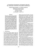
Figure 3 presents an image with 8 regions from the
database and the four corresponding segmentation results.
As we can see in this figure, these segmentation results have
different qualities.
The intrinsic qualit y of the segmentation results we used
for the comparison of evaluation criteria is not so important.
Indeed, we are looking for an unsupervised evaluation crite-
rion that has a similar behavior to a supervised one used as
reference (Vinet’s measure). A similar methodology concern-
ing performance measures for video object segmentation can
be found in [23].
Evaluation criteria
The tested unsupervised evaluation criteria for the compara-
tive study are
(i) the Borsotti criterion (BOR) [15],
(ii) the Zeboudj criterion (ZEB) [17],
(iii) the Rosenberger criteria: intra-inter (ROS 1) and adap-
tative criterion (ROS 2) [14],
(iv) the Levine and Nazif criteria: intra (LEV 1) and inter
(LEV 2) [24].
A good segmentation result maximizes the value of a cri-
terion, except for the Borsotti one that has to be minimized.
In order to facilitate the understanding of the proposed anal-
ysis, we used 1
− BOR(I
R

) as the Borsotti’s value instead of
BOR(I
R
) for each segmentation result I
R
.
The Vinet’s measure [6] that is a supervised criterion
which corresponds to the correct classification rate is used as
reference for the analysis of the synthetic images. In this case,
the ground truth is available. This criterion is often used to
compare a segmentation result I
R
with a ground truth I
R
ref
in
(a) (b)
(c) (d)
(e)
Figure 3: Example of an image with 8 regions and its segmentation
results: (a) original image, (b) fuzzy K-means, (c) fuzzy K-means +
relaxation, (d) EDISON, (e) ground tr uth.
the literature. We compute the following superposition table:
T

I
R
, I
R
ref


=

card

R
i
∩ R
ref
j

, i=1, , N
R
, j = 1, , N
R
ref

,
(14)
where card
{R
i
∩ R
ref
j
} is the number of pixels belonging to
the region R
i
in the segmentation result I
R

and to the region
R
j
in the ground truth.
With this table, we recursively search the matched classes
as illustrated in the Figure 4, for example, according to the
following method:
(1) we first select into the table the two classes that maxi-
mize card(R
i
∩ R
ref
j
),
(2) all the table elements that belong to the row and the
column of the mentioned cell are deselected,
(3) while there are elements left, we go back to the first
step.
According to the selected cells, Vinet’s measure gives a
dissimilarity measure. Let C

be the set of the selected cells,
6 EURASIP Journal on Applied Signal Processing
(a) (b) (c)
Figure 4: Computation of the Vinet measure: (a) segmentation re-
sult, (b) ground truth, (c) maximal overlapping result.
the Vinet measure is computed as follows:
VIN

I

R
, I
R
ref

=
Card(I) −

C

Card

R
i
∩ R
ref
j

Card(I)
. (15)
This criterion is often used to compute correct classifica-
tion rate of the segmentation result of a synthetic image.
3.2. Experimental results
In this section, we analyze the previously presented unsuper-
vised evaluation criteria. Their quality is evaluated by con-
sidering the comparison similarity with the Vinet measure
using their values on segmentation results.
Comparative study
We here look for the evaluation criteria having the most sim-
ilar behaviors to the Vinet one. In order to achieve this goal,

we consider the comparison results of the different segmen-
tation results for all the evaluation criteria. As we have four
segmentation results of each image, we have 6 p ossible com-
parisons. These 6 possible comparisons of four segmentation
results A, B, C, and D are A>B, A>C, A>D, B>C, B>D,
C>D. A comparison result is a value in
{0, 1}.Ifasegmen-
tation result has a higher value for the considered evaluation
criterion than another one, the comparison value is set to 1
otherwise it is set to 0. In order to define the similarity be-
tween each evaluation criterion and the Vinet measure, an
absolute difference is measured between the criterion com-
parison and the Vinet one. We define the cumulative similar-
ity of correct comparison (SCC) as follows:
SCC
=
8400

k=1
6

i=1


A(i, k) − B(i, k)


, (16)
where A(i, k) is the ith comparison result by using the Vinet
measure and B(i, k)byanevaluationcriterionfortheimage

k (1 <k<8400).
In order to quantify the efficiency of the evaluation cri-
teria, we define the similarity rate of correct comparison
Table 1: SRCC value of all the criteria with the Vinet measure for
different subsets of the image database with a fixed quantity of uni-
form and textured regions.
ZEB BOR LEV 1 LEV 2 ROS 1 ROS 2
BC100U 88.45% 65.73% 52.18% 73.72% 65.97% 50.70%
BC75U
67.31% 27.50% 40.80% 69.92% 39.98% 52.89%
BC50U
54.51% 19.21% 33.51% 71.83% 32.21% 55.80%
BC25U
38.78% 12.47% 25.71% 72.83% 25.80% 60.80%
BC0U
32.23% 11.10% 20.01% 74.61% 23.46% 64.98%
BC0UN
15.12% 11.20% 15.68% 33.62% 32.27% 61.33%
BCU 49.40% 24.53% 31.32% 66.09% 36.62% 57.75%
(SRCC), which represents the absolute similarity of compar-
ison with the Vinet measure referenced to the maximal value:
SRCC
=

1 −
SCC
SCC
max

∗

100, (17)
where SCC
max
= 6 × 8400 = 33 600 comparison results.
We can visualize in Ta ble 1 the SRCC value of all the crite-
ria with VIN. We can then note that ZEB and LEV 2 have the
strongest value of the SRCC in the case of uniform images. In
the textured case, LEV 2 is in first position followed by ROS 2
except for the B0UN group. When textured regions have the
same mean gray levels, ROS 2 provides better results.
The criteria which obtain the best values of the SRCC in
almost all cases are LEV 2, ZEB, and ROS 2. These three crite-
ria are complementary if we consider the type of the original
images. Indeed, the more the image contains textured (resp.,
uniform) regions, the more LEV 2 or ROS 2 (resp., ZEB) is
efficient.
We illustrate thereafter the behaviors of the different cri-
teria on various types of images.
Evaluation of segmentation results
We illustrate in this part, the behavior of these evaluation cri-
teria for different types of images. The Vinet measure (cor-
rect classification rate), considered as the reference, allows to
identify the best segmentation result.
Case of an uniform image. Figure 5 presents an original
image with only uniform regions and its four segmentation
results. In this case, VIN chooses the ground truth as being
the best followed by the EDISON result. As shown in Table 2,
only ZEB is able to sort these segmentation results like VIN.
Case of a mixed image. Figure 6 presents an original im-
age with unifor m and textured regions from BC50U and its

four segmentation results. According to Table 3 ,LEV2and
ROS 2 sort correctly the segmentation results except for one
comparison.
Caseofatexturedimage.Figure 7 presents an original
image with only textured regions from BC0U and its four
segmentation results. In this c ase, ROS 2 is the only criterion
that sorts correctly the segmentation results except for one
comparison (see Table 4).
Sebastien Chabrier et al. 7
Table 2: Values of the evaluation criteria computed on the segmentation results of Figure 5.
Segmentation result ZEB BOR LEV 1 LEV 2 ROS 1 ROS 2 VIN
FKM 0.6955 0.9995 0.0756 0.9835 0.5733 0.6551 0.7548
FKM + relaxation
0.7442 0.9996 0.0974 0.9904 0.5671 0.6328 0.9358
EDISON
0.8477 0.9997 0.5219 0.9833 0.5675 0.6628 0.9999
Ground truth
0.8478 0.9997 0.9833 0.5200 0.5675 0.6629 1.0000
(a) (b)
(c) (d)
(e)
Figure 5: One uniform image and its four segmentation results: (a)
original image, (b) FKM, (c) FKM + relaxation, (d) EDISON, (e)
ground truth.
Case of a textured image for regions with the same mean
gray level. Figure 8 presents an original image with only tex-
tured regions with the same mean gray-level from BC0UN
and its four seg mentation results. According to Table 5,only
ROS 2 sorts correctly the segmentation results. We can notice
that LEV 2 gives bad results in this case.

As a conclusion of this comparative study, ZEB has to
be preferred for uniform images while LEV 2 and ROS 2 are
more adapted for mixed and textured ones.
(a) (b)
(c) (d)
(e)
Figure 6: One image composed of uniform and textured regions
and its four segmentation results: (a) original image, (b) FKM, (c)
FKM + relaxation, (d) EDISON, (e) ground truth.
4. APPLICATION TO REAL IMAGES
We illustr a te here the ability of the previous evaluation crite-
ria to compare di fferent segmentation results of a single im-
age a t a same level of precision (here the number of classes).
Images chosen as illustration in this paper are an aerial and
a radar image (see Figure 9). They were segmented by three
different methods: FCM [25], PCM [20], and EDISON [21].
The first image corresponds to an aerial image composed
of uniform and textured regions (Figure 10). The majority
8 EURASIP Journal on Applied Signal Processing
Table 3: Values of the evaluation criteria computed on the segmentation results of Figure 6.
Segmentation result ZEB BOR LEV 1 LEV 2 ROS 1 ROS 2 VIN
FKM 0.6055 0.9996 0.9786 0.0388 0.5479 0.7069 0.6473
FKM + relaxation
0.4989 0.9994 0.9907 0.0368 0.5477 0.8005 0.6279
EDISON
0.6535 0.9990 0.9697 0.2747 0.5470 0.7529 0.9300
Ground truth
0.6530 0.9991 0.9718 0.3322 0.5475 0.8138 1.0000
(a) (b)
(c) (d)

(e)
Figure 7: One image composed of textured regions and its four segmentation results: (a) original image, (b) FKM, (c) FKM + relaxation,
(d) EDISON, (e) ground truth.
Table 4: Values of the evaluation criteria computed on the segmentation results of Figure 7.
Segmentation result ZEB BOR LEV 1 LEV 2 ROS 1 ROS 2 VIN
FKM 0.7145 0.9993 0.9806 0.0832 0.5465 0.5714 0.3687
FKM + relaxation
0.5528 0.9987 0.9865 0.1232 0.5446 0.7621 0.3981
EDISON
0.4076 0.9952 0.9510 0.1305 0.5324 0.8359 0.5549
Ground truth
0.3181 0.9913 0.9510 0.1018 0.5281 0.7796 1.0000
Sebastien Chabrier et al. 9
(a) (b)
(c) (d)
(e)
Figure 8: One image composed of textured regions with the same mean gray value and its four segmentation results: (a) original image, (b)
FKM, (c) FKM + relaxation, (d) EDISON, (e) ground truth.
Table 5: Values of the evaluation criteria computed on the segmentation results of Figure 8.
Segmentation result ZEB BOR LEV 1 LEV 2 ROS 1 ROS 2 VIN
FKM 0.7939 0.9998 0.9947 0.0379 0.5241 0.6696 0.2210
FKM + relaxation
0.5419 0.9994 0.9907 0.0449 0.5241 0.7003 0.2482
EDISON
0.5698 0.9990 0.9831 0.1167 0.5365 0.7733 0.2511
Ground truth
0.1979 0.9956 0.9692 0.0026 0.4956 0.7942 1.0000
of the criteria descr ibe the EDISON segmentation result as
being the best (Table 6). In our mind, this is also the case
visually.

The second image corresponds to a strongly noisy radar
image (see Figure 11). The regions can thus be regarded as
being all textured. Visually, the best segmentation result of
this image is, from our point of view, the EDISON one.
Table 7 presents it as being the best in almost all cases. ROS 2
gives to this segmentation result a much better quality score
compared to the FCM and PCM ones. On the contrary, ZEB
ranks very badly the EDISON segmentation result. More-
over, ZEB still keeps very weak values (
 0.1 whereas for
the segmentation results of the other images, the results ex-
ceeded 0.7 for the best). It confirms that ZEB is not adapted
to strongly textured images.
In order to validate these results on real images, one could
make a psychovisual study involving a significant number of
experts [8, 23].
10 EURASIP Journal on Applied Signal Processing
(a) (b)
Figure 9: Two real images: (a) radar image, (b) aerial image.
(a) (b)
(c) (d)
Figure 10: Three segmentation results of the aerial image: (a) original image, (b) FCM, (c) PCM, (d) EDISON.
5. CONCLUSION
Segmentation evaluation is essential to quantify the perfor-
mance of the existing segmentation methods. In this paper,
the majority of the existing unsupervised criteria for the
evaluation and the comparison of segmentation methods are
referred and presented. The present study tries to show the
strong points, the weak points, and the limitations of some
of these criteria.

For the comparative study, we used a large database com-
posed of 8400 synthetic images containing from 2 to 15 re-
gions. We thus have 33 600 segmentation results and con-
sequently 50 400 comparisons of segmentation results. We
could note that three criteria give better results than the
others:ZEB,LEV2,andROS2.ZEBisadaptedforuniform
Table 6: Values of the evaluation criteria computed on the segmen-
tation results of Figure 10.
Criterion FCM PCM EDISON
BOR 0.9888 0.9713 0.9945
ZEB
0.6228 0.6124 0.5428
LEV 1
0.7258 0.7112 0.9693
LEV 2
0.0901 0.0889 0.1099
ROS 1
0.5202 0.5239 0.5275
ROS 2
0.6379 0.6328 0.6973
images, while LEV 2 and ROS 2 find their applicability for
textured images.
Sebastien Chabrier et al. 11
(a) (b)
(c) (d)
Figure 11: Three segmentation results of the radar image: (a) orig-
inal image, (b) FCM, (c) PCM, (d) EDISON.
Table 7: Values of the evaluation criteria computed on the segmen-
tation results of Figure 11.
FCM PCM EDISON

BOR 0.9148 0.8207 0.9707
ZEB
0.1094 0.1172 0.0432
LEV 1
6.2846 7.5824 1.1364
LEV 2
0.1401 0.1394 0.2559
ROS 1
0.5196 0.5214 0.5419
ROS 2
0.4699 0.4677 0.9074
We illustrated the importance of these evaluation crite-
ria for the evaluation of segmentation results of real images
without any a priori knowledge. The selected criteria were
able, in our examples, to choose the segmentation result that
was visual ly perceived as being the best.
A prospect for this work is to combine the best criteria in
order to optimize their use in the various contexts. Perspec-
tives of this study concern the application of these evaluation
criteria for the choice of the segmentation method parame-
ters or the definition of new segmentation methods by opti-
mizing an evaluation criterion.
ACKNOWLEDGMENTS
The authors would like to thank the Conseil R
´
egional du
Centre and the European Union (FSE) for their financial sup-
port.
REFERENCES
[1]J.Freixenet,X.Mu

˜
noz, D. Raba, J. Marti, and X. Cufi, “Yet
another survey on image segmentation: region and boundary
information integration,” in Proceedings of the European Con-
ference on Computer Vision (ECCV ’02), pp. 408–422, Copen-
hagen, Denmark, May 2002.
[2] R. M. Haralick and L. G. Shapiro, “Image segmentation
techniques,” Computer Vision, Graphics, & Image Processing,
vol. 29, no. 1, pp. 100–132, 1985.
[3] Y. J. Zhang, “A survey on evaluation methods for image seg-
mentation,” Pattern Recognition, vol. 29, no. 8, pp. 1335–1346,
1996.
[4] N. M. Nasab, M. Analoui, and E. J. Delp, “Robust and efficient
image segmentation approaches using Markov random field
models,” Journal of Electronic Imaging, vol. 12, no. 1, pp. 50–
58, 2003.
[5] A. J. Baddeley, “An error metric for binary images,” in Robust
Computer Vision, pp. 59–78, Wichmann, Karlsruhe, Germany,
1992.
[6] L. Vinet, Segmentation et mise en correspondance de r
´
egions de
paires d’images st
´
er
´
eoscopiques, Ph.D. thesis, Universit
´
edeParis
IX Dauphine, Paris, France, 1991.

[7] D. P. Huttenlocher and W. J. Rucklidge, “Multi-resolution
technique for comparing images using the Hausdorff dis-
tance,” in Proceedings of IEEE Computer Vision and Pattern
Recognition (CVPR ’93), pp. 705–706, New York, NY, USA,
June 1993.
[8] D. Martin, C. Fowlkes, D. Tal, and J. Malik, “A database of hu-
man segmented natural images and its application to evaluat-
ing segmentation algorithms and measuring ecological statis-
tics,” in Proceedings of the IEEE International Conference on
Computer Vision (ICCV ’01), vol. 2, pp. 416–423, Vancouver,
BC, Canada, July 2001.
[9] J. S. Weszka and A. Rosenfeld, “Threshold evaluation tech-
niques,” IEEE Transactions on Systems, Man and Cybernetics,
vol. 8, no. 8, pp. 622–629, 1978.
[10] M. D. Levine and A. M. Nazif, “Dynamic measurement of
computer generated image segmentations,” IEEE Transactions
on Pattern Analysis and Machine Intelligence, vol. 7, no. 2, pp.
155–164, 1985.
[11] M. Sezgin and B. Sankur, “Survey over image thresholding
techniques and quantitative performance evaluation,” Journal
of Electronic Imaging, vol. 13, no. 1, pp. 146–168, 2004.
[12] W. G. Cochran, “Some methods for strengthening the com-
mon χ
2
tests,” Biometrics, vol. 10, pp. 417–451, 1954.
[13] N. R. Pal and S. K. Pal, “Entropic thresholding,” Signal Process-
ing, vol. 16, no. 2, pp. 97–108, 1989.
[14] C. Rosenberger, Mise en oeuvre d’un syst
`
eme adaptatif de

segmentation d’images, Ph.D. thesis, Universit
´
edeRennes1,
Rennes, France, 1999.
[15] M. Borsotti, P. Campadelli, and R. Schettini, “Quantita-
tive evaluation of color image segmentation results,” Pattern
Recognition Letters, vol. 19, no. 8, pp. 741–747, 1998.
[16] J. Liu and Y H. Yang, “Multiresolution color image segmen-
tation,” IEEE Transactions on Pattern Analysis and Machine In-
telligence, vol. 16, no. 7, pp. 689–700, 1994.
[17] R. Zeboudj, Filtrage, seuillage automatique, contraste et con-
tours: du pr
´
e-traitement
`
a l’analyse d’image, Ph.D. thesis, Uni-
versit
´
e de Saint Etienne, Saint Etienne, France, 1988.
[18]S.Chabrier,C.Rosenberger,H.Laurent,B.Emile,andP.
March
´
e, “Evaluating the segmentation result of a gray-level
12 EURASIP Journal on Applied Signal Processing
image,” in Proceedings of 12th European Signal Processing Con-
ference (EUSIPCO ’04), pp. 953–956, Vienna, Austria, Septem-
ber 2004.
[19]S.Chabrier,B.Emile,H.Laurent,C.Rosenberger,andP.
March
´

e, “Unsupervised evaluation of image segmentation ap-
plication to multi-spectral images,” in Proceedings of Interna-
tional Conference on Pattern Recognition (ICPR ’04), vol. 1, pp.
576–579, Cambridge, UK, August 2004.
[20] R. Krishnapuram and J. M. Keller, “Possibilistic c-means algo-
rithm: insights and recommendations,” IEEE Transactions on
Fuzzy Systems, vol. 4, no. 3, pp. 385–393, 1996.
[21] D. Comaniciu and P. Meer, “Mean shift: a robust approach
toward feature space analysis,” IEEE Transactions on Pattern
Analysis and Machine Intelligence, vol. 24, no. 5, pp. 603–619,
2002.
[22] H. A. Monawer, “Image vector quantization using a modified
LBG algorithm with approximated centroids,” Elect ronics Let-
ters, vol. 31, no. 3, pp. 174–175, 1995.
[23] C¸ . E. Erdem, B. Sankur, and A. M. Tekalp, “Performance mea-
sures for video object segmentation and tracking,” IEEE Trans-
actions on Image Processing, vol. 13, no. 7, pp. 937–951, 2004.
[24] A. M. Nazif and M. D. Levine, “Low level image segmentation:
an expert system,” IEEE Transactions on Pattern Analysis and
Machine Intelligence, vol. 6, no. 5, pp. 555–577, 1984.
[25] R. Krishnapuram and J. M. Keller, “Possibilistic approach to
clustering,” IEEE Transactions on Fuzzy Systems, vol. 1, no. 2,
pp. 98–110, 1993.
Sebastien Chabrier is an Assistant Profes-
sor at ENSI of Bourges (France). He ob-
tained his Ph.D. degree from the University
of Orleans in 2005. He works at the Labo-
ratory of Vision and Robotics, Bourges, in
the Signal, Image, and Vision Research Unit.
His research interests include segmentation

evaluation.
Bruno Emile is an Assistant Professor at
IUT of Chateauroux (France). He obtained
his Ph.D. degree from the University of Nice
in 1996. He works at the Laboratory of Vi-
sion and Robotics, Bourges, in the Signal,
Image, and Vision Research Unit. His re-
search interests include segmentation eval-
uation and object detection.
Christophe Rosenberger is an Assistant
Professor at ENSI of Bourges (France). He
obtained his Ph.D. degree from the Uni-
versity of Rennes I in 1999. He works
at the Laboratory of Vision and Robotics,
Bourges, in the Signal, Image, and Vision
Research Unit. His research interests in-
clude evaluation of image processing and
quality control by artificial vision.
Helene Laurent is an Assistant Professor at
ENSI of Bourges (France). She obtained her
Ph.D. degree from the University of Nantes
in 1998. She works at the Laboratory of Vi-
sion and Robotics, Bourges, in the Signal,
Image, and Vision Research Unit. Her re-
search interests include segmentation eval-
uation and pattern recognition.