Báo cáo hóa học: " Research Article Broadband Beamspace DOA Estimation: Frequency-Domain and Time-Domain Processing " potx

Hindawi Publishing Corporation
EURASIP Journal on Advances in Signal Processing
Volume 2007, Article ID 16907, 10 pages
doi:10.1155/2007/16907
Research Article
Broadband Beamspace DOA Estimation: Frequenc y-Domain
and Time-Domain Processing Approaches
Shefeng Yan
Institute of Acoustics, Chinese Academy of Sciences, 100080 Beijing, China
Received 1 November 2005; Revised 11 April 2006; Accepted 12 May 2006
Recommended by Peter Handel
Frequency-domain and time-domain processing approaches to direction-of-arrival (DOA) estimation for multiple broadband far
field signals using beamspace preprocessing structures are proposed. The technique is based on constant mainlobe response beam-
forming. A set of frequency-domain and time-domain beamformers with constant (frequency independent) mainlobe response
and controlled sidelobes is designed to cover the spatial sector of interest using optimal array pattern synthesis technique and
optimal FIR filters design technique. These techniques lead the resulting beampatterns higher mainlobe approximation accuracy
and yet lower sidelobes. For the scenario of strong out-of-sector interfering sources, our approaches can form nulls or notches in
the direction of them and yet guarantee that the mainlobe response of the beamformers is constant over the design band. Nu-
merical results show that the proposed time-domain processing DOA estimator has comparable performance with the proposed
frequency-domain processing method, and that both of them are able to resolve correlated source signals and provide better res-
olution at lower signal-to-noise ratio (SNR) and lower root-mean-square error (RMSE) of the DOA estimate compared with the
existing method. Our beamspace DOA estimators maintain good DOA estimation and spatial resolution capability in the scenario
of strong out-of-sector interfering sources.
Copyright © 2007 Hindawi Publishing Corporation. All rights reserved.
1. INTRODUCTION
Broadband direction-of-arrival (DOA) estimation has found
numerous applications to radar, sonar, wireless communica-
tions, and other areas. Incoherent signal-subspace methods
such as [1, 2] perform narrowband DOA estimation for each
frequency bin and then statistically combine the resulting es-
timates to form a broadband DOA estimate. However, co-

herent signal sources cannot be handled by this approach.
The coherent signal subspace (CSS) method was proposed
by Wang and Kaveh [3] as an alternative method to deal with
coherent signal sources. It decomposes the broadband data
into several narrowband frequency bins and finds focusing
matrices that transform the covariance matrices of each bin
into the one corresponding to the reference frequency bin.
Conventional narrowband D OA estimation methods such as
MUSIC [4] may then be directly applied to find the direc-
tions of arrival. CSS methods have been found to exhibit bet-
ter resolution at low signal-to-noise ratio (SNR) and lower
estimate variance than incoherent methods. However, the de-
sign of focusing matrices in the CSS method requires prelim-
inary DOA estimates in the neighborhood of the true direc-
tions of arrival.
Other broadband DOA estimation methods based on
the beamspace preprocessing are proposed in [5, 6]. The
beamspace preprocessing is performed by using frequency-
invariant beamformers (FIBs) that transform the ele-
mentspace into the beamspace. The beamforming matrices
perform the same operation as focusing matrices in the CSS
method, but without preliminary DOA estimates. In [5], Lee
constructs a beamforming matrix for each frequency bin
such that the resulting beampatterns are essentially identi-
cal for all frequencies by solv ing a least squares optimiza-
tion problem. However, the least squares fit is employed not
only in the mainlobe but also in the sidelobe regions, which
leads to suboptimal designs since the sidelobes only need
to be guaranteed to remain below the prescribed threshold
value. In [6], Ward et al. present a DOA estimator that per-

forms broadband focusing using time-domain processing,
in which a set of appropriately designed beam-shaping fil-
ters [7] ensure that the similar array pattern is produced for
all frequencies within the design band. The estimator need
not perform frequency decomposition. However, the FIBs
may not be achieved for arrays with arbitrary geometry and
nonuniform interelement spacing. Moreover, it is difficult to
control the mainlobe width and sidelobe level. Furthermore,
2 EURASIP Journal on Advances in Signal Processing
the robustness of the beamformers designed in [5, 6]may
decrease since the beamforming weights can be very large.
We will refer to the beamspace preprocessing approaches in
[5, 6] as frequency-domain f requency-invariant beamspace
(FD-FIBS) approach and time-domain frequency-invariant
beamspace (TD-FIBS) approach, respectively.
In this paper, new broadband DOA estimation ap-
proaches are proposed by designing a set of frequency-
domain and time-domain beamformers with constant main-
lobe response over the design band to cover the spatial sector
of interest. We will refer to the beamformer with constant
mainlobe response as constant mainlobe response beamformer
(CMRB). The frequency-domain weight vector of CMRB is
designed using optimal array pattern synthesis techniques
to ensure that the resulting beampattern is constant within
the mainlobe over the design band while guarantee the side-
lobes to be below the prescribed values. For our array pattern
synthesis problems, the least squares fit process is only per-
formed within the mainlobe, which can lead to higher main-
lobe approximation accuracy. For our time-domain beam-
former, a bank of FIR filters corresponding to the input chan-

nels are designed to provide the frequency responses that ap-
proximate the frequency-domain array weights for each sen-
sor. Both the array pattern synthesis and the FIR filter de-
sign problems are formulated as the second-order cone pro-
gramming (SOCP), which can be solved efficiently using the
well-developed interior-point methods [8, 9]. The SOCP ap-
proach has been exploited in robust array interpolation [10]
and robust beamforming [11, 12]. The proposed DOA esti-
mators are a ble to resolve correlated source signals and can
be applicable to arrays of arbitrary geometry. For the sce-
nario of strong out-of-sector interfering sources, our esti-
mators can maintain good DOA estimation and spatial res-
olution capability by forming nulls or notches in the corre-
sponding directions and yet guarantee that the mainlobe re-
sponse of the broadband beamformer is constant over the
design band.
The paper is organized as follows. A brief review of
broadband beamspace DOA estimation is presented in
Section 2.InSection 3, the frequency-domain and time-
domain CMRBs are designed using SOCP approach. In
Section 4, the frequency-domain and time-domain process-
ing methods for beamspace DOA estimation are presented.
Section 5 presents simulation results confirming the effi-
ciency of the proposed methods, and Section 6 concludes the
paper.
2. BACKGROUND
Consider an N-element array with a known arbitrary geome-
try. Assume that D<Nfar field broadband sources impinge
on the array from directions Θ
= [θ

1
, , θ
d
, , θ
D
]. The
time series received at the nth element is
x
n
(t) =
D

d=1
s
d

t − ξ
n

θ
d

+ v
n
(t), n = 1, , N,(1)
where s
d
(t) is the dth source signal, ξ
n
(θ

d
) is the propagation
delay to the nth sensor associated with the dth source, and
v
n
(t) is the additive white noise. With suitable data segmen-
tation and Fourier transform, the frequency response of the
N
× 1 complex array data snapshot vector is g iven by
x

f
j

=
A

Θ, f
j

s

f
j

+ v

f
j


,(2)
where the argument f
j
denotes the dependence of the array
data on different frequency bins, s( f
j
) = [s
1
( f
j
), , s
D
( f
j
)]
T
is the D ×1 source signal vector. Here (·)
T
denotes the trans-
pose. v( f
j
) is the N ×1 additive noise vector, and A(Θ, f
j
) =
[a(θ
1
, f
j
), , a(θ
D

, f
j
)] is the N × D source direction ma-
trix with a(θ
d
, f
j
) = [e
−i2πf
j
ξ
1
(θ
d
)
, , e
−i2πf
j
ξ
N
(θ
d
)
]
T
(d =
1, , D) being the array manifold vector. Here i =
√
−1.
In beamspace eigen-based methods, multiple beams are

formed over the spatial sector of interest by using a set
of K (D<K<N) beamforming weight vectors w
jk
=
[w
1
( f
j
, k), , w
n
( f
j
, k), , w
N
( f
j
, k)]
T
, j = 1, , J, k =
1, , K.Herew
n
( f
j
, k) is the weight of the kth beamformer
associated with the nth sensor employed at the frequency bin
f
j
. Assume that the pointing directions of the K beamform-
ers are Φ
= [φ

1
, , φ
k
, , φ
K
]. The received elementspace
data snapshot vectors are converted into a reduced dimen-
sion beamspace data snapshot vector via the matrix transfor-
mation
y

f
j

= W
H
j
x

f
j

= W
H
j
A

Θ, f
j


s

f
j

+ W
H
j
v

f
j

=
B

Θ, f
j

s

f
j

+ v
B

f
j


,
(3)
where B(Θ, f
j
) = W
H
j
A(Θ, f
j
)andv
B
( f
j
) = W
H
j
v

f
j

are
the beamspace DOA matrices and noise vectors, respectively.
Here (
·)
H
denotes the Hermitian transpose. And W
j
=
[w

j1
, w
j2
, , w
jK
] is the N × K beamforming matrices em-
ployed at the frequency bin f
j
.
Assume that we apply the constant (frequency indepen-
dent) mainlobe response b eamforming technique. Then the
response of the beamformer may be made approximately
constant within the mainlobe over the design band, that is,
p
k

θ, f
j

=
w
H
jk
a

θ, f
j

≈
p

CMR,k
(θ),
j
= 1, , J, k = 1, , K, θ ∈ Θ
M
,
(4)
where p
CMR,k
(θ) is the constant mainlobe response associ-
ated with the kth beamformer, Θ
M
is the mainlobe angular
region, in contrast to the methods in [5, 6], where the beam-
formers are designed to ensure that the resulting beampat-
tern is constant over both the mainlobe and the sidelobe re-
gions.
Because the constant response property of the beam-
formers, the beamspace DOA matrices are approximately
constant for al l frequencies, that is,
B

Θ, f
j

≈
B(Θ), j = 1, , J. (5)
Hence, the broadband source directions are completely char-
acterized by a single beamspace DOA matrix B(Θ).
Shefeng Yan 3

Assuming the source signals and the noise are uncorre-
lated, the constant mainlobe response beamspace (CMRBS)
data covariance matr ix is
R
y

f
j

=
E

y

f
j

y
H

f
j

=
B(Θ)E

s

f
j


s
H

f
j

B
H
(Θ)
+ W
H
j
E

v

f
j

v
H

f
j

W
j
= B(Θ)R
s


f
j

B
H
(Θ)+R
v

f
j

,
(6)
where R
s
( f
j
) = E{s ( f
j
)s
H
( f
j
)}is the D×D source covariance
matrix, and R
v
( f
j
) = W

H
j
E{v( f
j
)v
H
( f
j
)}W
j
is the K × K
CMRBS noise covariance matrix. The broadband CMRBS
data covariance matrix can be formed as
R
y
=
J

j=1
R
y

f
j

=
J

j=1


B(Θ)R
s

f
j

B
H
(Θ)

+
J

j=1
R
v

f
j

=
B(Θ)

J

j=1
R
s

f

j


B
H
(Θ)+R
v
,
(7)
where R
v
=

J
j
=1
R
v
( f
j
) is the broadband beamspace noise
covariance matrix.
The broadband CMRBS data covariance matrix (7)is
now in a form in which conventional eigen-based DOA es-
timators may be applied. Denote the eigen-decomposition of
matrix pencil (R
y
, R
v
) as (see also [3])

R
y
E = ΛR
v
E,(8)
where Λ is the diagonal matrix of sorted eigenvalues, E
=
[E
s
, E
v
] contains the corresponding eigenvectors with E
s
and
E
v
being the eigenvectors corresponding to the largest D
eigenvalues and to the smallest K–D eigenvalues, respec-
tively.
For the MUSIC algorithm [4], the source directions are
given by the D peak positions of the following spatial spec-
trum:
P(θ)
=
b
H
(θ)b(θ)
b
H
(θ)E

v
E
H
v
b(θ)
,(9)
where b(θ) is the transformed steering vector in beamspace.
It is defined as b(θ)
= W
H
( f )a(θ, f )forsome f = f
j
, j =
1, , J.
3. DESIGN OF CONSTANT MAINLOBE
RESPONSE BEAMFORMER
Concentrate on one of the K beamformers, for example, the
kth beamformer, and omit the k symbol temporarily for con-
venience. The other beamformers can be designed by the
same procedure.
3.1. Frequency-domain beamformer
For a reference beampattern, it is preferable to employ beam-
formers exhibiting high gain within the desired spatial sec-
tor and yet uniformly low sidelobes in order to suppress un-
wanted out-of-sector interfering sources. Let f
0
be the refer-
ence frequency, which need not be one of f
j
( j = 1, , J).

Let θ
s
∈ Θ
S
(s = 1, , S)andθ
m
∈ Θ
M
(m = 1, , M)be
a chosen grid that approximates the sidelobe region Θ
S
,and
the mainlobe region Θ
M
, respectively, using a finite number
of angles. The design of reference beampattern, say p
d
(θ, f
0
),
can be stated as
min
w
0
w
H
0
R
n
w

0
,
subject to p
d

φ
0
, f
0

=
1,


p
d

θ
s
, f
0



≤
δ, ∀θ
s
∈ Θ
S
,

(10)
where w
0
is the optimal weight vector, that is, design vari-
able, and p
d
(θ, f
0
) = w
H
0
a(θ, f
0
), R
n
is the noise covariance
matrix at the reference frequency f
0
which becomes an iden-
tity matrix for the special case of spatially white noise, φ
0
is
the pointing direction of the beamformer, and δ is the pre-
scribed sidelobe value.
The optimal weight vector employed at the frequency bin
f
j
,sayw
j0
, can be obtained by solving the following least

squares optimization problem:
min
w
j0

M

m=1


p
d

θ
m
, f
o

−
p

θ
m
, f
j



2


, θ
m
∈ Θ
M
,
subject to


p

θ
s
, f
j



≤
δ
s
, ∀θ
s
∈ Θ
S
,
w
j0


≤

Δ,
(11)
where p(θ, f
j
) = w
H
j0
a(θ, f
j
) is the so-obtained beampattern
at the frequency bin f
j
, δ
s
(s = 1, , S) are the desired side-
lobe values which can be prescribed to satisfy various re-
quirements. It can even be prescribed to provide nulls or
notches to suppress strong out-of-sector interferences. The
constraint
w
j0
≤Δ limits the white-noise gain to improve
the beamformer robustness against random errors in array
characteristics [13].
The optimization problems (10)and(11)canbeformu-
lated as the SOCP problem, which can be efficiently solved
using the well-established interior point algorithms, for ex-
ample, by SeDuMi MATLAB toolbox [8]. A review of the ap-
plications of SOCP can be found in [9].
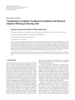
3.2. Time-domain beamformer

Time-domain broadband beamformers can be implemented
by placing a tapped delay line or FIR filter at the output of
each sensor [14–16]. Each sensor feeds an FIR filter and the
filter outputs are summed to produce the beam output time
series. In a time-domain CMRB, the sensor filters perform
the role of beam shaping and ensure that the beam shape is
constant as a function of frequency within the mainlobe.
Assume that the FIR filter associated with the nth sensor
is h
n
= [h
n
(1), , h
n
(l), , h
n
(L)]
T
.HereL is the length of
4 EURASIP Journal on Advances in Signal Processing
Sensors Delays
FIR
filter h
1
FIR
filter h
N
Output
.
.

.
.
.
.
.
.
.
.
.
.
Optimal design of FIR filters
1
N

τ
1
(φ
0
) T
s
τ
N
(φ
0
) T
s
Figure 1: FIR broadband beamformer structure.
the filter and h
n
is a real vector. Its corresponding frequency

response at frequency f
j
is H
n
( f
j
), and should equal approxi-
mately the array weight w
n
( f
j
)employedatfrequency f
j
.The
key problem of the time-domain broadband beamformer is
how to design the FIR filters.
The inherent group delay (unit in taps) of an FIR filter of
length L is nearly ( L
− 1)/2. The group delay of the desired
FIR filter is not exactly equal to (L
− 1)/2 in general, and
can b e decomposed into an integer part plus a decimal part.
We assume that the needed presteering delay (unit in taps)
that aligns the desired signal arrived from φ
0
(the pointing
direction of the beamformer) for channel n is ζ
n
(φ
0

). The
array weight can be thus rewritten as [17]
w
n

f
j

= e
−i2πf
j
int[ζ
n
(φ
0
)−(L−1)/2]T
s
· w
n

f
j

e
i2πf
j
int[ζ
n
(φ
0

)−(L−1)/2]T
s
,
(12)
where T
s
is the sampling interval and int[·]denotesround
towards nearest integer. The first part of (12) can be imple-
mented by a tapped delay-line delay of τ
n
(φ
0
) = int[ζ
n
(φ
0
) −
(L −1)/2] taps (when it is minus, a plus integral number can
be added for all channels), and the second part by an FIR
filter. Thus, the desired frequency response of an FIR filter
associated with the nth sensor can be expressed as
H
n,d

f
j

= w
n


f
j

e
i2πf
j
τ
n
(φ
0
)T
s
,
j
= 1, 2, , J, n = 1, 2, , N,
(13)
The structure of FIR broadband beamformer with pointing
direction φ
0
is shown in Figure 1.
The complex frequency response corresponding to the
impulse response h
n
is given by
H( f )
=
L

l=1
h

n
(l)e
−i(l−1)2πf/f
s
= e
T
( f )h
n
, (14)
where e( f )
= [1, e
−i2πf/f
s
, , e
−i(L−1)2πf/f
s
]
T
and f
s
is the
sampling frequency.
Let F
p
be the stopband, which is discretized using a finite
number of frequencies f
p
∈ F
P
(p = 1, 2, , P). The design

problem of FIR filter associated with the nth sensor is then
stated as
min
h
n

J

j=1


H
n,d

f
j

−
e
T

f
j

h
n


2


,
subject to


e
T

f
p

h
n


≤
ε, ∀f
p
∈ F
P
,
(15)
where ε is the prescribed stopband attenuation.
The optimization problems ( 15 ) can also be formulated
as a second-order cone programming problem. An SOCP-
based solving procedure for an FIR filter design can be found
in our earlier paper [18].
4. CONSTANT MAINLOBE RESPONSE BEAMSPACE
DOA ESTIMATION
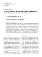
4.1. Frequency-domain processing
The frequency-domain processing structure for DOA estima-

tion is shown in Figure 2(a). Assume we a pply CMRBs to the
received array data in frequency domain. The K-dimensional
time series of the K conjunctive beamformer outputs at the
frequency bin f
j
is given by
y

f
j
, q

=
W
H
j
x

f
j
, q

, (16)
where q is the snapshot index. The K
× K beamspace data
covariance matrix of the K beamformer outputs at the fre-
quency bin f
j
can be estimated from the data vector y( f
j

, q)
over a finite series of snapshots q
= 1, 2, , Q,

R
y
( f
j
) =
1
Q
Q

q=1

y

f
j
, q

y
H

f
j
, q

, (17)
The broadband beamspace data covariance matrix is then

constructed by coherently combining the sample covariance
matrices

R
y
=
J

j=1

R
y

f
j

. (18)
Assuming the element space noise covariance matrix,
that is, E
{v( f
j
)v
H
( f
j
)}, is known, then the broadband
beamspace noise covariance matrix can be formed as
R
v
=

J

j=1

W
H
j
E

v

f
j

v
H

f
j

W
j

. (19)
In the specific case in which the noise is spatially white
and uncorrelated from sensor to sensor, the beamspace noise
covariance matr ix is
R
v
=

σ
2
J
J

j=1

W
H

f
j

W

f
j

, (20)
where σ
2
is the noise power. If W is not unitary, then the
noise will get colored after multiplication with W.
Shefeng Yan 5
x
1
(t)
x
2
(t)

x
N
(t)
BufferBufferBuffer
FFTFFTFFT
x( f
1
)
x( f
2
)
x( f
J
)
x( f
1
)
x( f
2
)
x( f
J
)
x( f
1
)
x( f
2
)
x( f

J
)
w
11
w
21
w
J1
w
12
w
22
w
J2
w
1K
w
2K
w
JK
y( f
1
)

R
y
( f
1
)


R
y
( f
2
)

R
y
( f
J
)

R
y
R
v
.
.
.
.
.
.
.
.
.
.
.
.
.
.

.
.
.
.
.
.
.
.
.
.
Narrowband DOA estimator (e.g., MUSIC)
(a)
Delays Filters
x
1
(t)
x
2
(t)
x
N
(t)
y
1
(t)
y
K
(t)




τ
1
(φ
1
) T
s
τ
2
(φ
1
) T
s
τ
N
(φ
1
) T
s
τ
1
(φ
2
) T
s
τ
2
(φ
2
) T

s
τ
N
(φ
2
) T
s
τ
1
(φ
K
) T
s
τ
2
(φ
K
) T
s
τ
N
(φ
K
) T
s
h
11
h
21
h

N1
h
12
h
22
h
N2
h
1K
h
2K
h
NK

R
y
R
v
.
.
.
.
.
.
.
.
.
.
.
.

.
.
.
Narrowband DOA estimator (e.g., MUSIC)
(b)
Figure 2: Broadband DOA estimation using CMRBs. (a) Frequency-domain processing structure. (b) Time-domain processing structure.
4.2. Time-domain processing
The time-domain processing structure for DOA estima-
tion is shown in Figure 2(b).Leth
nk
= [h
nk
(1), , h
nk
(l) ,
h
nk
(L)]
T
be the filter associated with the nth sensor employed
at the kth beamformer. The time series of the kth beam-
former output is given by
y
k
(t) =
N

n=1
L


l=1
h
nk
(l)x
n

t − (l − 1) − τ
n
(φ
k
)

, (21)
where t is the time index.
The K-dimensional time series of the K conjunctive
beamformeroutputsisgivenby
y(t)
=

y
T
1
(t), , y
T
k
(t), , y
T
K
(t)


T
, (22)
where
y
k
(t) is the discrete-time analytic signal of y
k
(t), which
can be obtained via a Hilbert transform. Note that since fo-
cusing is performed by a set of FIR filters in the time do-
main, it is unnecessary to perform frequency decomposition
in order to form the beamspace data covariance matrix. The
broadband beamspace data covariance matrix can be formed
from the K-dimensional beamformer outputs over a finite
time period t
= 1, 2, , T.

R
y
=
1
T
T

t=1

y(t)y
H
(t)


. (23)
From (13), we see that the virtual beamforming weights
employed at frequency f associated with the nth sensor and
the kth beamformer is
w
n
( f ,k) = H
nk
( f )e
−i2πfτ
n
(φ
k
)T
s
, (24)
where H
nk
( f ) = e
T
( f )h
nk
is the resulting frequency response
of the FIR filters associated with the nth sensor and the kth
beamformer.
The broadband beamspace noise covariance matrix can
now be formed as
R
v
=


f
U
f
L

W
H
( f )E

v( f )v
H
( f )


W( f )df , (25)
where

W( f ) =
⎡
⎢
⎢
⎢
⎣

w
1
( f ,1) ··· w
1
( f ,K)

.
.
.
.
.
.
.
.
.
w
N
( f ,1) ··· w
N
( f ,K)
⎤
⎥
⎥
⎥
⎦
(26)
is the virtual N
× K beamforming matrix and [ f
L
, f
U
]is
the design band. The integral operation can be represented
approximately in a sum form by discretizing the frequency
band.
In the specific case in which the noise is spatially white

and uncorrelated from sensor to sensor, the broadband
beamspace noise covariance matrix is
R
v
=
σ
2
f
U
− f
L

f
U
f
L

W
H
( f )

W( f )df. (27)
4.3. Summary of DOA estimation algorithms
We will refer to the proposed frequency-domain and time-
domain constant mainlobe response beamspace processing
DOA estimators as the FD-CMRBS approach and the TD-
CMRBS approach, respectively.
An outline of the FD-CMRBS broadband DOA estimator
is given as follows.
6 EURASIP Journal on Advances in Signal Processing

(1) Design K reference beamformers (10) and then K CM-
RBs (11) that cover the spatial region of interest.
(2) Calculate the broadband beamspace noise covariance
matrix R
v
(19)or(20).
(3) Calculate the K-dimensional beamformer outputs at
each frequency bin (16), and estimate the broadband
beamspace data covariance matrix

R
y
(18) from the
beamformer outputs over a finite snapshot period.
(4) Estimate the DOA of the sources from

R
y
and R
v
us-
ing a conventional narrowband DOA estimator such as
MUSIC (9).
For the FD-CMRBS DOA estimator, the beamform-
ing matrix can be calculated offline, and the broadband
beamspace noise covariance matrix needs only to be cal-
culated once, also offline, if the noise covariance does not
change over the observation time.
An outline of the TD-CMRBS broadband DOA estimator
is given as follows.

(1) Design K reference beamformer (10) and then K CM-
RBs (11) that cover the spatial region of interest.
(2) Calculate the desired frequency response of the FIR
filters associated with each sensor for each of the K
beamformers from frequency-domain weight vectors
(13), and then design the filters (15).
(3) Calculate the v irtual beamforming weights (24)from
the FIR filters.
(4) Calculate the broadband beamspace noise covariance
matrix R
v
(25)or(27).
(5) Calculate the K-dimensional time series of the K
beamformer outputs (22), and estimate the broadband
beamspace data covariance matrix

R
y
(23) from the
beamformer outputs over a finite time period.
(6) Estimate the DOA of the sources from

R
y
and R
v
us-
ing a conventional narrowband DOA estimator such as
MUSIC (9).
For the TD-CMRBS DOA estimator, the FIR filters can

be calculated offline, and the broadband beamspace noise co-
variance matrix can also be calculated once, also off line.
4.4. Computational complexities
The major computational demand of the broadband
beamspace DOA estimators comes from the implementation
of broadband beamformers.
For the frequency-domain implementation, we assume
the FFT length is , which is assumed to be a power of 2. The
computation of the FFT for the data obtained from all the N
sensors requires a computational complexity of N × ×log
2

complex multiplications. In the weight-and-sum stage, to
form K beams, it requires a complexity of N
×J ×K complex
multiplication. The overall complexity of frequency-domain
broadband beamforming for a block of  data samples is
N
×  × log
2
 + N ×J × K complex multiplication.
If the percentage of the overlap among the input blocks
is α, the overall complexity will be (N
×  × log
2
 + N ×
J ×K)/(1 −α) complex multiplication. If the sliding window
technique is used, in which the FFT is computed each time
a new sample enters the buffer, the complexity of frequency-
domain broadband beamforming for the  data samples will

be (N
×  × log
2
 + N ×J × K) × complex multiplication.
For the time-domain implementation, the beam output
time series is produced when each new data sample arrives,
in contrast to the FFT beamformer, which requires a block
of samples to perform the FFT. Since the tap weights of the
FIR filters are real, to form K beams, the overall complex-
ity of time-domain broadband beamforming for the  data
samples is N
×  × L × K real multiplication, in which the
computational complexity of a real multiplication is 4 times
less than that of a complex multiplication.
Therefore, if the parameters are chosen to be some rea-
sonable values (such as those used in Section 5), the time-
domain implementation has a higher computational com-
plexity as compared to the frequency-domain implementa-
tion without overlap, while less than that of the frequency-
domain implementation with the sliding window technique.
5. SIMULATIONS
5.1. DOA estimation for correlated sources
Consider a linear array of N
= 15 uniformly spaced el-
ements, with a half-wavelength spacing at the center fre-
quency, also chosen as the reference frequency, f
0
= 0.3125
(The normalized sampling frequency was 1). The normal-
ized design band [ f

L
, f
U
] = [0.25, 0.375] is decomposed
into J
= 33 uniformly distributed subbands. K = 4CM-
RBs are designed to cover the spatial sector [0
◦
,22.5
◦
]with
respect to the broadside of the array, that is,
{φ
k
}
4
k
=1
=
{
0
◦
,7.5
◦
,15
◦
,22.5
◦
}. The corresponding beampatterns at all
the 33 frequency bins are shown in Figure 3(a).Thevaria-

tion with frequency of the beampattern directed towards 0
◦
is
shown in Figure 3(b), from which it is seen that the resulting
beampattern within the mainlobe is approximately constant
over the frequency band and the sidelobes are strictly guaran-
teed to be below
−30 dB. Just as we desired, the SOCP-based
optimal array pattern synthesis approach provides small syn-
thesized errors to CMRBs.
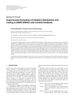
The desired frequency response of the FIR filters associ-
ated with each sensor for each beamformer is calculated from
the array weights via (13 ). The desired magnitude and phase
responses within the design band associated with the 5th sen-
sor for the first beamformer is shown in Figure 3(c) (with
“
·”). Assume that the length of each FIR filter is L = 64.
By solving the optimization problem (15), the magnitude
and phase responses of the resulting FIR filter are shown in
Figure 3(c). Similar results were obtained for the other FIR
filters.
The beampatterns of the time-domain FIR beamformer
are calculated at the same 33 frequency bins and shown in
Figure 3(d), from which it is seen that the mainlobe response
of the resulting beampattern is approximately constant over
the entire design band. The time-domain broadband CMRB
is implemented with satisfying beampatterns. The sidelobes
are just a little higher than that of the frequency-domain
Shefeng Yan 7
9060300306090

Angle (deg)
80
70
60
50
40
30
20
10
0
Beampatterns (dB)
(a)
90
60
30
0
30
60
90
Angle (deg)
0.25
0.275
0.3
0.325
0.35
0.375
Normalized frequency
60
40
20

0
Beampatterns (dB)
(b)
0.50.40.30.20.10
50
40
30
20
10
Amplitude (dB)
0.50.40.30.20.10
Normalized frequency
200
100
0
100
200
Phase (deg)
Desired
Designed
(c)
9060300306090
Angle (deg)
80
70
60
50
40
30
20

10
0
Beampatterns (dB)
(d)
Figure 3: Design of the CMRBs. (a) Superposition of the beampatterns of frequency-domain CMRBs in K = 4 directions at J = 33
frequencies. (b) Variation of beampattern with frequency for the beamformer of 0
◦
. (c) Frequency response of the FIR filter associated with
the 5th sensor of the first beamformer. (d) Superposition of the beampatterns of time-domain CMRBs in K
= 4 directions calculated at
J
= 33 frequencies.
beampatterns since there exist some errors, which are very
small and acceptable, b etween the desired and the designed
filters.
A set of simulations was performed to compare the
performance of the proposed FD-CMRBS and TD-CMRBS
DOA estimators with the FD-FIBS DOA estimator proposed
by Lee in [5]. Signals from two correlated sources arrived
at θ
1
= 8
◦
and θ
2
= 11
◦
. The first source signal is as-
sumed to be a bandpass white Gaussian process with flat
spectral density over the design band. The second source

signal is a delayed version of the first one. The delay at the
first sensor (the spatial reference point) is 10T
s
. A spatially
white Gaussian bandpass noise with flat spectral density, in-
dependent of the received signals, was present at each array
element. The received data was decomposed into J
= 33 fre-
quency bins using an unwindowed FFT of length 
= 256.
For our frequency-domain processing approach, 30 snap-
shots were used to calculate each DOA estimate. Thus, a total
of 256
×30 = 7680 data samples were used for each DOA esti-
mation. The same amount of data samples was used for each
DOA estimator. The conventional MUSIC DOA estimator is
used on the beamformer outputs for each approach.
Figure 4 shows the spatial spectra of the three broad-
band beamspace DOA estimators when the SNR is 6 dB. All
the approaches are able to resolve the correlated source sig-
nals. Our TD-CMRBS DOA estimator has comparable per-
formance w ith our FD-CMRBS estimator, and, as expected,
both of them outperform the FD-FIBS.
8 EURASIP Journal on Advances in Signal Processing
302520151050510
Angle (deg)
60
50
40
30

20
10
0
MUSIC spatial spectrum (dB)
FD-FIBS
FD-CMRBS
TD-CMRBS
Figure 4: DOA estimation result for two correlated sources using FD-FIBS, FD-CMRDS, and TD-CMRDS.
201001020
SNR (dB)
0
0.2
0.4
0.6
0.8
1
Probability of resolution
FD-FIBS
FD-CMRBS
TD-CMRBS
(a)
201510505
SNR (dB)
0
0.1
0.2
0.3
0.4
0.5
RMSE (deg)

FD-FIBS
FD-CMRBS
TD-CMRBS
CRB
(b)
Figure 5: Performance comparison of FD-FIBS, FD-CMRBS, and FD-CMRBS for several SNR values. (a) Comparison of the resolution
performance. (b) Compar ison of the RMSEs.
The probability of resolution versus SNR for the two
sources is shown in Figure 5(a). Results are based on 100 in-
dependent trials for each SNR, using the same array data for
each approach. The signal sources are said to be resolved in a
trial if [19]
2

d=1



θ
d
− θ
d


<


θ
1
− θ

2


, (28)
where

θ
d
is the DOA estimate of the dth source in the trial.
The resulting sample root-mean-squared error (RMSE)
of the DOA estimate of the source at θ
1
= 8
◦
, obtained from
100 independent trials, is shown in Figure 5(b). These re-
sults also show that the performance of TD-CMRBS is com-
parable with that of FD-CMRBS, and that our approaches
exhibit better resolution performance than that of FD-FIBS.
Also plotted in Figure 5(b) is the square root of Cramer-Rao
bound (CRB) of the source at 8
◦
, which is numerically calcu-
lated by the procedure given in the appendix of [3]. The RM-
SEs of our DOA estimators (FD-CMRBS and TD-CMRBS)
are seen to be very close to the square root of CRB, which
confirm the efficiency of the proposed methods.
Shefeng Yan 9
60300306090
Angle (deg)

0
5
10
15
20
25
30
Signal/interference-to-noise (dB)
Interfering source
Two correlated sources
(a)
60300306090
Angle (deg)
40
35
30
25
20
15
10
5
0
MUSIC spatial spectrum (dB)
(b)
9060300306090
Angle (deg)
80
70
60
50

40
30
20
10
0
Beampatterns (dB)
(c)
60300306090
Angle (deg)
60
50
40
30
20
10
0
MUSIC spatial spectrum (dB)
(d)
Figure 6: DOA estimation for the scenario of strong out-of-sector interfering source. (a) Directions of the two correlated sources and the
interfering source. (b) DOA estimation result using the beamformers with uniform sidelobes. (c) Superposition of the notch beampatterns.
(d) DOA estimation result using the notch beamformers.
5.2. Interference rejection via notch beamformers
Consider the scenario of strong out-of-sector interfering
sources. For the above linear array, the two correlated sources
arrived at 8
◦
and 11
◦
with SNR = 6 dB. An interfering source,
independent of the wanted sources, arrived at

−54
◦
with
the interference-to-noise ratio (INR) of 26 dB, as shown in
Figure 6(a).
Figure 6(b) shows the spatial spectrum of beamspace
MUSIC using the beamformers shown in Figure 3(a).Itis
seen that the CMRBs with uniformly sidelobe level of
−30 dB
cannot resolve the correlated sources in the scenario of strong
out-of-sector interfering sources.
The K
= 4 CMRBs that cover the same spatial sector
[0
◦
,22.5
◦
] are designed by setting a notch with the depth of
−60 dB and the width of 4
◦
in the direction of the interfering
source. The resulting beampatterns are shown in Figure 6(c),
from which it is seen that the mainlobe response is constant
over the design band and the prescribed notch is formed on
each beampattern. The MUSIC DOA estimation method is
used on the K beamformer outputs. The spatial spectrum
of the frequency-domain processing approach is shown in
Figure 6(d), from which it is seen that our approach is able
to resolve correlated source signals in the scenario of strong
out-of-sector interfering sources.

6. CONCLUSION
Frequency-domain and time-domain processing approaches
to broadband beamspace coherent signal subspace DOA es-
timation using constant mainlobe response beamforming
have been proposed. Our approaches can be applicable to
arrays of arbitrar y geometry. SOCP-based time-domain and
10 EURASIP Journal on Advances in Signal Processing
frequency-domain broadband beamformers with constant
mainlobe response are designed. The MUSIC method is then
applied to the beamformer outputs to perform the DOA
estimation. Computer simulations results show that our
frequency-domain and time-domain broadband beamspace
DOA estimators exhibit better resolution performance than
the existing method. Our DOA estimators maintain good
DOA estimation and spatial resolution capability in the sce-
nario of strong out-of-sector interfering sources by setting a
notch in the direction of the interfering source.
ACKNOWLEDGMENT
This project was supported by China Postdoctoral Science
Foundation.
REFERENCES
[1] G. Su and M. Morf, “The signal subspace approach for multi-
ple wide-band emitter location,” IEEE Transactions on Acous-
tics, Speech, and Signal Processing, vol. 31, no. 6, pp. 1502–
1522, 1983.
[2] M. Wax, T J. Shan, and T. Kailath, “Spatio-temporal spec-
tral analysis by eigenstructure methods,” IEEE Transactions on
Acoustics, Speech, and Signal Processing, vol. 32, no. 4, pp. 817–
827, 1984.
[3] H. Wang and M. Kaveh, “Coherent signal-subspace process-

ing for the detection and estimation of angl es of arrival of
multiple wide-band sources,” IEEE Transactions on Acoustics,
Speech, and Signal Processing, vol. 33, no. 4, pp. 823–831, 1985.
[4] R. O. Schmidt, “Multiple emitter location and signal param-
eter estimation,” IEEE Transactions on Antennas and Propaga-
tion, vol. 34, no. 3, pp. 276–280, 1986.
[5] T S. Lee, “Efficient wideband source localization using beam-
forming invariance technique,” IEEE Transactions on Signal
Processing, vol. 42, no. 6, pp. 1376–1387, 1994.
[6] D. B. Ward, Z. Ding, and R. A. Kennedy, “Broadband DOA
estimation using frequency invariant beamforming,” IEEE
Transactions on Signal Processing, vol. 46, no. 5, pp. 1463–1469,
1998.
[7] D. B. Ward, R. A. Kennedy, and R. C. Williamson, “FIR fil-
ter design for frequency invariant beamformers,” IEEE Signal
Processing Letters, vol. 3, no. 3, pp. 69–71, 1996.
[8] J. F. Sturm, “Using SeDuMi 1.02, a MATLAB toolbox for op-
timization over symmetric cones,” Optimization Methods and
Software, vol. 11, no. 1, pp. 625–653, 1999.
[9] M. S. Lobo, L. Vandenberghe, S. Boyd, and H. Lebret, “Appli-
cations of second-order cone programming,” Linear Algebra
and Its Applications, vol. 284, no. 1–3, pp. 193–228, 1998.
[10] M. Pesavento, A. B. Gershman, and Z Q. Luo, “Robust array
interpolation using second-order cone programming,” IEEE
Signal Processing Letters , vol. 9, no. 1, pp. 8–11, 2002.
[11] S. A. Vorobyov, A. B. Gershman, and Z Q. Luo, “Robust adap-
tive beamforming using worst-case performance optimiza-
tion: a solution to the signal mismatch problem,” IEEE Trans-
actions on Signal Processing, vol. 51, no. 2, pp. 313–324, 2003.
[12] S. Yan and Y. L. Ma, “Robust supergain beamforming for

circular array via second-order cone programming,” Applied
Acoustics, vol. 66, no. 9, pp. 1018–1032, 2005.
[13] H. Cox, R. Zeskind, and M. Owen, “Robust adaptive beam-
forming,” IEEE Transactions on Acoustics, Speech, and Signal
Processing, vol. 35, no. 10, pp. 1365–1376, 1987.
[14] R. T. Compton Jr., “The relationship between tapped delay-
line and FFT processing in adaptive arrays,” IEEE Transactions
on Antennas and Propagation, vol. 36, no. 1, pp. 15–26, 1988.
[15] L. C. Godara, “Application of the fast Fourier t ransform to
broadband beamforming,” Journal of the Acoustical Society of
America, vol. 98, no. 1, pp. 230–240, 1995.
[16] H. L. Van Trees, Detection, Estimation, and Modulation Theory,
Part IV, Optimum Array Processing, John Wiley & Sons, New
York, NY, USA, 2002.
[17] S. Yan, “Optimal design of FIR beamformer with frequency
invariant patterns,” Applied Acoustics, vol. 67, no. 6, pp. 511–
528, 2006.
[18] S. Yan and Y. L. Ma, “A unified framework for designing FIR
filters with arbitrary magnitude and phase response,” Digital
Signal Processing, vol. 14, no. 6, pp. 510–522, 2004.
[19] A. B. Gershman, “Direction finding using beamspace root es-
timator banks,” IEEE Transactions on Signal Processing, vol. 46,
no. 11, pp. 3131–3135, 1998.
Shefeng Yan received the B.S., M.S., and
Ph.D. degrees in electr ical engineering
from Northwestern Polytechnical Univer-
sity, Xi’an, China, in 1999, 2001, and 2005,
respectively. He is currently a Postdoctoral
Fellow with the Institute of Acoustics, Chi-
nese Academy of Sciences, Beijing, China.

His current research interests include array
signal processing, statistical signal process-
ing, adaptive signal processing, optimiza-
tion techniques, and signal processing applications to underwater
acoustics, radar, and wireless mobile communication systems. He
is a member of IEEE.