Báo cáo hóa học: " Research Article Statistical Analysis of Hyper-Spectral Data: A Non-Gaussian Approach" pot

Hindawi Publishing Corporation
EURASIP Journal on Advances in Signal Processing
Volume 2007, Article ID 27673, 10 pages
doi:10.1155/2007/27673
Research Article
Statistical Analysis of Hyper-Spectral Data:
A Non-G aussian Approach
N. Acito, G. Corsini, and M. Diani
Dipartimento di Ingegneria dell’Informazione, Universit
`
a di Pisa, Via Caruso, 14-56122 Pisa, Italy
Received 5 June 2006; Revised 9 October 2006; Accepted 24 October 2006
Recommended by Ati Baskurt
We investigate the statistical modeling of hyper-spectral data. The accurate modeling of experimental data is critical in target de-
tection and classification applications. In fact, having a statistical model that is capable of properly describing data variability leads
to the derivation of the best decision strategies together with a reliable assessment of algorithm performance. Most existing clas-
sification and target detection algorithms are based on the multivariate Gaussian model which, in many cases, de viates from the
true statistical behavior of hyper-spectral data. This motivated us to investigate the capability of non-Gaussian models to represent
data variability in each background class. In particular, we refer to models based on elliptically contoured (EC) dist ributions. We
consider multivariate EC-t distribution and two distinct mixture models based on EC distributions. We describe the methodology
adopted for the statistical analysis and we propose a technique to automatically estimate the unknown parameters of statistical
models. Finally, we discuss the results obtained by analyzing data gathered by the multispectral infrared and visible imaging spec-
trometer (MIVIS) sensor.
Copyright © 2007 N. Acito et al. This is an open access article distributed under the Creative Commons Attribution License, which
permits unrestricted use, distribution, and reproduction in any medium, provided the original work is properly cited.
1. INTRODUCTION
The main characteristic of hyper-spectral sensors is their
ability to acquire a spectral signature of the monitored area,
thus enabling a spectroscopic analysis to be carried out of
large regions of terrain.
The large amount of data collected by hyper-spectral sen-

sors can lead to an improvement in the performance of de-
tection/classification algorithms. Within this framework, it
is important to note that the spectral reflectance of the ob-
served object is not a deterministic quantity, but is character-
ized by an inherent variability determined by changes in the
surface of the objec t. In remote sensing applications, spec-
trum variability is emphasized by several factors, such as at-
mospheric conditions, sensor noise, and acquisition geome-
try. One possible way to properly address the spectral vari-
ability is to make use of suitable statistical models. Although
the statistical approach has benefits both in classification and
detection applications, in this paper, we focus on target de-
tection problems. By using a statistical approach, the generic
hyper-spectral pixel x is modeled as an L-dimensional ran-
dom vector (where L is the number of sensor spectral chan-
nels) that is a certain multivariate probability density func-
tion (p.d.f.). Target detection reduces to a binary classifica-
tion problem, where by observing x one must decide if it
belongs to the background class (H
0
hypothesis) or to the
target class (H
1
hypothesis) by using an appropriate decision
rule. The availability of a multivariate model that properly
accounts for the statistical behavior of hyper-spectral data
leads to
(1) the derivation of the “best” decision rule,
(2) the analytical derivation of the detector’s performance.
The derivation of the algorithms’ performance is a criti-

cal issue in designing automatic target detection systems and
is a fundamental tool for defining the criteria for a correct
choice of algorithm parameters.
Most of the detection algorithms proposed in the litera-
ture (see [1, 2]) and widely used in current applications have
been derived under the multivariate Gaussian assumption.
The popularity of the Gaussian model is due to its math-
ematical tractability. In fact, it simplifies the derivation of
decision rules and the evaluation of the detectors’ perfor-
mance. Unfortunately, the multivariate Gaussian model is
not sufficiently adequate to represent the statistical behavior
of each background class in real hyperspectral images. It has
been proved (see [3–5]) that the Gaussian model fails in its
representation of the distribution tails. In particular, current
2 EURASIP Journal on Advances in Signal Processing
distributions have longer tails than the Gaussian p.d.f. This
is a critical issue in detection applications. In fact, the dis-
tribution tails determine the number of false alarms. Most
detection applications require the algorithm test threshold
to be set in order to control the probability of false alarms
(P
FA
). Generally, parameters are set on the basis of the P
FA
predicted by the model adopted to describe the data. Since
the Gaussian model underestimates the distribution tails, the
parameter tuning based on such a model could be mislead-
ing in that the actual number of false alarms might exceed
the desired number.
To overcome the limits of the Gaussian model in de-

scribing the statistical behavior of background classes in
real hyper-spectral images, in recent years multivariate non-
Gaussian models have been investigated. A very promising
class of models is the family of the elliptically contoured dis-
tributions (ECD) [4, 5]. It has some statistical properties that
simplify the analysis of multidimensional data and includes
several distributions that have longer tails than the Gaussian
one.
In this paper, we focus on three distinct probability mod-
els based on the ECD theory. ECD models were proposed
in two recently published papers (see [4, 5]), where the au-
thors applied the multivariate EC-t distribution, a particu-
lar class of ECD family, to model data gathered by the HY-
DICE sensor. They showed that there is a good agreement
between the probability distribution estimated over HYDICE
data and the theoretical one derived by assuming the EC-
t model. In particular, by resorting to the properties of the
EC distributions the authors compared the probability of ex-
ceedance (PoE) of the square of the Mahalanobis distance ob-
tained over real data with the theoretical PoE. For the EC-t
distribution, the PoE of the square of the Mahalanobis dis-
tance depends on a scalar value υ.In[4, 5] the authors graph-
ically showed that by varying υ the curve corresponding to
the theoretical PoE tends to the empirical one; they did not
address the important problem of automatically estimating
the value of υ from the available data.
In this study, first we apply the hyper-spectral data anal-
ysis proposed in [5] and based on the EC-t distribution in
order to model data collected by the MIVIS (multispectral
infrared and visible imaging spectrometer) sensor. We ex-

tend the analysis procedure further by defining two different
methods to estimate the parameter υ. One of our proposed
techniques estimates υ directly from the available data. This
makes the method very interesting for practical applications
where the background parameters included in the algorithm
decision rules must be estimated directly from the analyzed
image.
Furthermore, we also analyse experimental data vari-
ability by using mixture models so as to take into account
the spatial or spectral nonhomogeneity in the background
classes considered. In particular, we investigate the effective-
ness of mixture models whose p.d.f. is obtained as a linear
combination of EC p.d.f.’s (see [6]). We consider two distinct
mixture models, and we define a technique to automatically
estimate their unknown parameters.
The paper is organised as follows: first, we introduce the
ECD and we describe in detail the three models considered
in our analysis; then, for each model we illustrate the tech-
nique used to estimate the unknown parameters. Finally, we
present and discuss the results obtained by analyzing two dis-
tinct background classes in an MIVIS image.
2. NON-GAUSSIAN MODELS
2.1. Elliptically contoured distribution
The L-dimensional random vector X
= [X
1
, X
2
, , X
L

]isEC
distributed, or equivalently it is a spherically invariant ran-
dom vector (SIRV) if its p.d.f. can be expressed as
f
x
(x) =
1
(2π)
L/2
|C|
1/2
h
L
(d), (1)
wherewedenotewithd the generic realization of the random
variable D corresponding to the square of the Mahalanobis
distance:
D
= (X − µ)
T
C
−1
(X − µ)(2)
and µ and C are the mean vector and the covariance matrix,
respectively.
ECDs have some important statistical properties as fol-
lows:
(1) the isolevel curves in (1) are elliptical;
(2) each vector obtained from the element of an SIRV is
also EC distributed;

(3) the p.d.f. of each set of variables
{X
i
: i ∈ I, I ∈
[1, , L]} conditioned to {X
j
: j ∈ J, J ∪ I =
[1, , L]} is an EC distribution;
(4) the maximum likelihood (ML) estimates of the param-
eters µ and Γ obtained from K samples x
k
of X can be
expressed as
µ =
1
K
K

k=1
x
k
,

C =
1
K
K

k=1


x
k
− µ

·

x
k
− µ

T
.
(3)
Furthermore, on the basis of the Yao representation theorem
[7], an SIRV can be expressed as
X
= AC
1/2
Z + µ,(4)
where Z is an L-dimensional Gaussian distributed random
vector with zero mean and identity covariance matrix, and
A is a scalar nonnegative random variable with unit squared
mean value. The two variables Z and A are statistically inde-
pendent.
According to (4), the p.d.f. of X is strictly related to the
statistical distribution of the scalar random variable A.In
particular, X conditioned to A has a multivariate Gaussian
distribution:
f
X|A

(x | α) =
1
(2π)
L/2
|C|
1/2
α
L
exp

−
d
2α
2

. (5)
N. Acito et al. 3
As a consequence, according to the principle of total proba-
bility, the p.d.f. of X can be written as
f
x
(x) =

∞
0
f
x|A
(x | α) · f
A
(α)dα

=
1
(2π)
L/2
|C|
L/2

∞
0
α
−L
exp

−
d
2α
2

f
A
(α)dα.
(6)
The p.d.f. of A is called the SIRV characteristic p.d.f.
Equations (1)and(6) prove that the function h
L
(d)isre-
lated to the characteristic p.d.f. of X by means of the following
integral equation:
h
L

(d) =

∞
0
α
−L
exp

−
d
2α
2

f
A
(α)dα. (7)
Thus, the statistical properties of X are uniquely determined
by the mean vector µ, the covariance matrix Γ and the uni-
variate p.d.f. of A.
The relationship between h
L
(d) and the p.d.f. f
D
(d)ofD
is (see [8, 9])
h
L
(d) =
2
L/2

L
L/2 −1
Γ(L/2)
d
L/2 −1
f
D
(d). (8)
Equations (6)and(7) are very useful in the statistical analysis
of the SIRVs. In fact, by assuming perfect knowledge of the
mean and covariance matrix of X, the analysis of the SIRV
multivariate p.d.f. reduces to the study of a univariate p.d.f.
In (8) the function h
L
(d) must be a nonnegative monotoni-
cally decreasing function (see [8]); thus, the statistical distri-
bution of D must satisfy this constraint and cannot be chosen
arbitrarily.
The class of EC distributions includes the multivariate
Gaussian model. In fac t, a Gaussian variable is an SIRV with
f
A
(α) = δ(α − 1),
h
L
(d) = exp

−
d
2


.
(9)
Tosummarize,anECmodelcanbedefinedbyspecifyingthe
multivariate p.d.f. of X, or the p.d.f. of the scalar random
variable D or by specifying the characteristic p.d.f. ( f
A
(α)).
In the latter two cases, knowledge of the mean vector and of
the covariance matrix must be assumed.
2.2. Models adopted
2.2.1. Elliptically contoured t distribution model
The first model is based on multivariate EC-t distribution
(see [4–6]). According to the EC-t model, the p.d.f. of X is
expressed as
f
x
(x)=
Γ

(L + ν)/2

Γ[ν/2](νπ)
L/2
|R|
−1/2

1+
1
ν

(x
−µ)
T
R
−1
(x−µ)

−L+ν/2
,
(10)
where R is related to the covariance matrix of X by the fol-
lowing equation:
R
=
υ − 2
υ
C. (11)
For the EC-t distribution, the scalar variable D can be ex-
pressed as
D
= L
υ
− 2
υ
Ω. (12)
In (12) Ω denotes an F-central random variable with L and υ
degrees of freedom. The parameter υ is strictly related to the
shape of the distribution tails. In particular, for υ
= 1, the
EC-t distribution reduces to the multivariate Cauchy distri-

bution that has heavy tails, whereas when υ
−∞it tends to the
multivariate Gaussian distribution characterized by lighter
tails.
In [4, 5] the authors analyzed background classes includ-
ing a number of pixels large enough to neglect the errors in
the estimate of the mean vector and the covariance matrix.
Thus, they reduced the analysis of the statistical behavior of
real data to the study of the univariate distribution of D.Note
that, by assuming perfect knowledge of µ and C, the EC-t dis-
tribution depends on the parameter υ alone. The analysis of
HYDICE data was carried out in terms of a graphical com-
parison between the empirical PoE and the theoretical one. In
particular, the authors showed that by varying the value of υ
the theoretical PoE of D tends to the empirical one. They did
not provide any method to automatically estimate the value
of υ to obtain the best fitting.
The analysis of the statistical behavior of MIVIS data was
carried out by also considering mixture models. The intro-
duction of those models has a physical rationale in the spa-
tial/spectral nonhomogeneity of the considered background
classes. In particular, we considered models whose p.d.f.’s
are expressed as a linear combination of ECD (see [6]). The
models adopted are characterized by one or more parame-
ters whose values must be set in order to obtain the best fit-
ting between the empirical p.d.f. and the theoretical one. In
mixture models, the number of parameters and the complex-
ity of their estimation process increase with the number of
component functions. One of the advantages of defining a
multivariate model, that properly describes the statistical be-

havior of real background classes, is the ability to derive op-
timum detection strategies. Consequently, it is important to
use models that are as simple as possible and that only have a
few parameters.
For these reasons in our analysis, we considered two
classes of mixture models that have few parameters and that
are characterized by a high mathematical tractability. Thus,
there is no physical meaning in the selected models. The
models considered are denoted as Gaussian mixture model
(GMM) [10]andN lognormal mixture model (N-LGM).
2.2.2. Gaussian mixture model (GMM)
The GMM exploits the fact that the distribution of hyper-
spectral data for a specific backg round class is obtained as the
linear combination of a finite number N of Gaussian func-
tions. In particular, the p.d.f. of X can be expressed as
f
GMM
(x) =
N

i=1
π
i
f
G

x; µ
i
, C
i


, (13)
4 EURASIP Journal on Advances in Signal Processing
where f
G
(x; µ
i
, C
i
) denotes the multivariate Gaussian p.d.f.
with mean vector µ
i
and covariance matrix C
i
and the π
i
∈
[0, 1] are the mixture weights subject to the sum to one con-
straint:

N
i=1
π
i
= 1. Thus, the whole set of model parameters
is Θ
≡{π
i
, µ
i

, C
i
, i = 1, , N}.
2.2.3. N-lognormal mixture model (N-LGM)
The N-LGM arises from the assumption that the p.d.f. of a
background class can be expressed as the linear combination
of ECD that share the same mean vector µ and covariance
matrix C and that have a lognormal characteristic p.d.f. The
model reduces to an SIRV with mean vector µ, covariance
matrix C,andcharacteristic p.d.f. expressed as the linear com-
bination of lognormal functions:
f
A
(α) =
N

i=1
π
i
f
(i)
A
(α), π
i
∈ [0, 1],
N

i=1
π
i

= 1,
f
(i)
A
(α) =
1
√
2πσ
i
α
exp

−
1
2σ
2
i

ln

α
δ
i

2

.
(14)
In (14) N denotes the number of mixture components and π
i

the mixture coefficients. By using (8), the p.d.f. of the square
of the Mahalanobis distance can be expressed as
f
D
(d) =
d
L/2 −1
2
L/2
Γ(L/2)
N

i=1
π
i

∞
0
α
−L
exp

−
d
2α
2

f
(i)
A

(α)dα.
(15)
According to the properties of the SIRV, since the variable A
had a unit mean squared value, we must set the following
constraints in the model (14):
δ
i
=−2σ
2
i
∀i ∈ [1, N]. (16)
Thus, by assuming that µ and C are known, the N-LGM is
characterized by the following set of parameters:
Θ
≡

c
1
, c
2
, , c
N
, π
1
, π
2
, , π
N−1

, (17)

where π
N
= 1 −

N−1
i=1
π
i
.
3. EXPERIMENTAL DATA ANALYSIS
To analyze the statistical behavior of experimental hyper-
spectral data, we assume that a certain number M of pix-
els
{x
1
, x
2
, , x
M
} of a specific background class is available.
Then x
i
can be obtained by applying a classification algo-
rithm to the image or by resorting to the ground truth if it is
available. The non-Gaussian models considered in this study
are characterized by one or more parameters that must be
properly set in order to fit the empirical probability distribu-
tion (i.e., the distribution estimated over real data). For each
of the three models, we propose a methodolog y to estimate
the parameters from the available data.

3.1. Elliptically contoured t distribution model:
parameter e stimation
For the ECD models, we resor t to (3)and(6)whichrep-
resent the relationships between the multivariate p.d.f. of
the data and the univariate distribution of the square of the
Mahalanobis distance. The model estimates are obtained by
considering the set
{d
i
: i = 1, , M;(x
i
− µ)
T
C
−1
(x
i
− µ)},
where µ and C are the mean vector and the covariance matrix
of the background class. In practice, µ and C are unknown
and must be estimated from the data. In our experiments,
we analyzed background classes including a large number of
pixels (larger than 10L), thus, the estimates of µ and C can be
reasonably considered as the exact values.
With regard to the EC-t model, the parameter υ must be
tuned to the empirical distribution. For this purpose, we pro-
pose two different techniques. The first one consists in setting
the unknown parameter to its ML estimate from the d
i
s. It is

obtained by looking for the value of υ that maximizes the
log-likelihood function defined as
log Λ

d
1
, d
2
, , d
M
, υ

=
M
i

k=1
log

f
D

d
k
; υ

,
f
D
(d; υ) =

υ
υ − 2
·
1
L
· f
Ω

d · υ
υ − 2
·
1
L

,
(18)
where f
Ω
(·) represents the p.d.f. of an F-central distributed
random variable with L and υ degrees of freedom. In eval-
uating the log-likelihood function, we assume the d
i
sare
samples drawn from M random variables that are mutu-
ally independent and identically distributed. Unfortunately,
the ML estimate of υ cannot be obtained in closed form, so
we resort to a numerical method to search for the absolute
maximum of the likelihood function. For this purpose, sev-
eral techniques can be adopted such as simulated annealing,
stochastic sampling methods, and genetic algorithms. In this

study, we adopted a genetic algorithm (GA) that uses the float
representation [11]. This algorithm is efficient for numerical
computations and is superior to both the binary genetic al-
gorithm and the simulated annealing in terms of efficiency
and quality of the solution (see [11]).
Note that, generally, in detection applications, in order
to evaluate the test statistic in the algorithm decision rule,
the background parameters must be estimated from a limited
data set representing the background class where the target of
interest is embedded. For this reason, the proposed estima-
tion technique can be very useful in practical applications.
In fact, it allows us to estimate the background parameter υ
from the samples d
i
s taken from the analyzed image.
In order to test the reliability of such an estimator, several
computer simulations were performed. In particular, in our
simulations we investigated the properties of the ML estima-
tor for different values of the parameter υ and of the num-
ber N
S
of samples used to evaluate the log-likelihood func-
tion. These samples were generated according to (12), and
the number of spectral bands L was set to 52 in accordance
with the characteristics of the MIVIS data adopted in the ex-
perimental analysis described in Section 4. Table 1 shows the
estimator mean values with respect to the number of sam-
ples and for each value of the parameter υ. Whereas, Ta ble 2
shows the estimator mean relative squared error versus the
N. Acito et al. 5

Table 1: ML estimator: mean values obtained by simulation. Re-
sults obtained considering 10
4
realizations of the ML estimator.
N
S
υ 10
2
10
3
10
4
10
5
5 5,001 5 5 5
20
20,051 20,014 20 20
50
50,259 50,059 50,007 50
80
80,279 80,198 80,06 80,001
Table 2: ML estimator: mean squared error obtained by simulation.
Results obtained considering 10
4
realizations of the ML estimator.
N
S
υ 10
2
10

3
10
4
10
5
5 10
−5
00 0
20
3, 5 · 10
−3
4 ·10
−4
00
50
6, 6 · 10
−3
7 ·10
−4
10
−4
1, 02 · 10
−5
80 7, 6 · 10
−3
14 ·10
−4
2 ·10
−4
1, 2 · 10

−5
number of samples. Note that for N
S
> 10
4
the estimator
mean reaches the true value of the parameter for each υ,and
the estimator mean relative squared error is less than 2
·10
−4
.
This leads us to conclude that the proposed estimator is un-
biased and consistent for N
S
> 10
4
. These results are in accor-
dance with the asymptotical properties of the ML estimators
(MLE). In fact, the MLEs are asymptotically unbiased, con-
sistent and efficient (they achieve the Cramer-Rao bound)
[12].
The second technique proposed to estimate the param-
eter υ in the EC-t model consists in searching for the “best
fitting” between the empirical and the theoretical cumulative
distribution functions (c.d.f.). The goodness of fit is evalu-
ated by a suitable cost function J
P
(υ) calculated on P selected
points (percentile) of the two c.d.f.’s and the estimate
υ is ob-

tained as
υ = min
υ

J
P
(υ)

,
J
P
(υ) =
P

k=1

log
10

F
emp

d
k

−
log
10

F

th

d
k
, υ

log
10

F
emp

d
k


2
.
(19)
In (19)wedenotewithF
emp
(·) the empirical c.d.f. de-
rived from the histogram of the d
i
sandwithF
th
(·, υ) the the-
oretical c.d.f. of the square of the Mahalanobis distance with
respect to the parameter υ. The cost function evaluates the
relative squared error between the logarithm of the empiri-

cal and theoretical c.d.f.’s. The logarithmic transformation is
applied in order to give the same weig ht to the body and to
the tails of the distributions. Since there is no closed form
solution for the optimization problem in (19), we resort to a
numerical method. In particular, we use the simplex search
method described in [13]. This is a direct search method that
does not use numerical or analytic gradients.
3.2. Gaussian mixture model: parameters estimation
With regard to the GMM, it is important to note that by
increasing the number N of functions in the mixture, one
would expect that the quality of the fitting would improve.
Unfortunately, the increase in the number of mixture ele-
ments also increases the complexity of the model and limits
its applicability to the analysis of the data and to the deriva-
tion of detection algorithms tuned to the statistical model.
For these reasons, we considered the two distributions ob-
tained by setting N
= 2 (2-GMM) and N = 3 (3-GMM).
The parameters of each multivariate Gaussian function and
the mixture weights are estimated directly from x
i
using the
expectation maximization (EM) algorithm [14].
3.3. N-lognormal mixture model:
parameter estimation
For the N-LGM, the parameter estimates are obtained using
an approach similar to the one in (19). In this case, we search
for the set of values

Θ that minimizes the cost function J

P
(Θ)
defined as
J
P
(Θ) =
P

k=1

log
10

f
emp

d
k

−
log
10

f
th

d
k
, Θ


log
10

f
emp

d
k


2
,
(20)
where f
emp
(·) denotes the empirical p.d.f. derived from the
histogram of the d
i
sand f
th
(·, Θ) indicates the theoretical
p.d.f. of the square of the Mahalanobis distance with respect
to the parameter vector Θ:
f
th
(d; Θ) = Hd
L/2−1

∞
0

a
−L
exp

−
d
2a
2

f
N−LGM
A
(a; Θ)da,
H
=
1
2
L/2
Γ(L/2)
.
(21)
Regarding the number of elements of the mixture we can
extend the remarks proposed for the GMM to the N-LGM.
Thus, to limit the complexity of the model, we considered
two mixture components (2-LGM).
4. EXPERIMENTAL RESULTS
The non-Gaussian models were applied to a set of real re-
flectance data in order to check which was the most appropri-
ate to fi t the empirical distribution. The data were collected
during a measurement campaign held in Italy in 2002. The

aim of the campaign was to collect data to support the de-
velopment and the analysis of classification and detection al-
gorithms. The data were gathered by the MIVIS instrument,
an airborne sensor with 102 spectral channels covering the
spectral region from the visible (VIS) to the thermal infrared
(TIR).
In this study, we refer to a reduced data set consisting
of 52 spectral channels selected by discarding the 10 TIR
channels and those characterized by low signal-to-noise ra-
tio (SNR). Furthermore, the SWIR channels were binned to
enhance the SNR. The ground resolution is about 3 m.
6 EURASIP Journal on Advances in Signal Processing
(a)
Class 1: grass
Class 2: bare soil
(b)
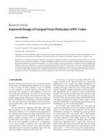
Figure 1: (a) RGB representation of the analyzed scene; (b) back-
ground classes considered.
Table 3: Number of pixels in each class.
Class no.1 Class no.2
Number of pixels 369951 23482
The results outlined in this paper regard two specific
background classes selected from an MIVIS image using
the unsupervised segmentation algorithm in [15]. The two
classes are labelled as class no.1 and class no.2 and they cor-
respond to two distinct regions of the scene covered by grass
and bare soil, respectively. In Figure 1, we show the RGB im-
age of the analyzed scene and we point out the two back-
ground classes considered. The number of pixels in each class
is listed in Ta ble 3. Since the number of pixels in each class is

far larger than the number of sensor spectral channels, it is
reasonable to assume that the errors in the mean vector and
in the covariance matrix estimates from the class pixels are
negligible. Thus, according to the properties of the ECDs, the
analysis of the statistical behavior of real data can be reduced
to the study of the distributions of the scalar variable D.
Theanalysiswascarriedoutintermsofagraphicalcom-
parison between the empirical distributions and the theoret-
ical ones. In Figures 2 and 3, the PoE of D estimated over
real data associated with the two classes (empirical PoE)are
compared with the PoE derived from each theoretical model
(theoretical PoE). The PoE is defined as
PoE(d)
= 1 −

d
0
f
D
(t)∂t, (22)
where f
D
(·) represents the p.d.f. of D. In plotting the PoE,we
used the logarithmic scale in order to highlight the distribu-
tion tail.
In Figures 2 and 3, the PoE obtained by assuming the
Gaussian model for the multivariate data has also been plot-
10
0
10

1
10
2
10
3
10
4
PoE
50 100 150 200
D
Real data
EC-t (ν
= 22)
EC-t (ν
ML
= 56)
2-GMM
3-GMM
2-LGM
χ
2
Figure 2: Class no.1 (grass): PoE of D for the real data and for the
theoretical models.
ted. In this case, assuming perfect knowledge of the class
mean vector and covariance matrix, the random variable D
has a central χ
2
distribution with L degrees of freedom.
The results confirm that the Gaussian model does not ac-
curately describe the statistical behavior of the data. In par-

ticular, it strongly deviates from the tails of the empirical dis-
tributions.
With regard to the EC-t model, we plotted two distribu-
tions for each class. The EC-t distributions were obtained by
setting the υ parameter to the values
υ
ML
and υ obtained by
the MLE and by the procedure that minimizes the cost func-
tion in (19), respectively. In each class, the EC-t distribution
derived by setting υ
= υ
ML
does not properly account for
the statistical behavior of the data. In particular, there is a
good agreement between the body of the empirical distri-
bution and the theoretical model but the distribution tail is
not properly modeled. Instead, the EC-t model obtained for
υ
= υ fits the empirical distribution tail well but it is not
completely appropriate for representing its body. The best
performances achieved by the EC-t model with υ
= υ
ML
in
fitting the body of the empirical distributions are more evi-
dent in Figures 4 and 5.Hereweplotted,forclass no.1 and
class no.2, the empirical p.d.f. of D and the theoretical ones.
In both the experiments discussed in this section the num-
ber of samples adopted to estimate the parameter υ using

the MLE is larger than 10
4
. Thus, according to the proper-
ties of the MLE we can state that if the pixels of each class
were drawn from an EC-t distribution,
υ
ML
would be a re-
liable estimate of the model parameter. This leads us to the
N. Acito et al. 7
10
0
10
1
10
2
10
3
10
4
PoE
20 40 60 80 100 120 140
D
Real data
EC-t (ν
= 39)
EC-t (ν
ML
= 81)
2-GMM

3-GMM
2-LGM
χ
2
Figure 3: Class no.2 (bare soil): PoE of D for the real data and for
the theoretical models.
conclusion that the statistical behavior of MIVIS data in the
two considered background classes is not fully represented by
means of an EC-t distribution. Furthermore, the fact that it is
possible to properly describe the body and the tail of empir-
ical distribution with two distinct EC-t models suggests that
the use of mixture models is more appropriate to properly
address hyper-spectral data variability. This has its physical
rationale in the spectral/spatial nonhomogeneity within the
observed background classes.
It is worth noting that the results suggest that the mul-
tivariate EC-t distribution cannot be adopted to derive op-
timum detection strategies. Nevertheless, they confirm that
the tails of the empirical dist ribution of real hyper-spectral
data can be properly represented by means of an EC-t model.
The a bility of EC-t models to follow the empirical distribu-
tion tails makes them very useful in assessing detection per-
formance. In particular, since in detection applications the
distribution tails are related to the number of false alarms,
the EC-t models facilitate the derivation of criteria for tun-
ing the algorithms, based on reliable predictions of the P
FA
.
With regard to the mixture models, the 2-GMM a nd the
3-GMM perform better than the Gaussian model but they

still do not provide a good representation of the data statis-
tical distribution. Also note that by increasing the number of
mixture elements from two to three, the results for fitting the
empirical distribution do not improve significantly.
Among the statistical models considered, the 2-LGM
provides the best performance in fitting the empirical dis-
tributions. In fact, it is totally suitable for representing the
body of the distributions for both classes, as is proved by the
results shown in Figures 4 and 5. Furthermore, Figure 3 high-
0.035
0.03
0.025
0.02
0.015
0.01
0.005
0
p.d.f
0 50 100 150 200 250
D
Real data
EC-t (ν
= 22)
EC-t (ν
ML
= 56)
2-LGM
Figure 4: Class no.1 (grass): p.d.f.’s for the real data and for three
theoretical models.
0.035

0.03
0.025
0.02
0.015
0.01
0.005
0
p.d.f
20 40 60 80 100 120 140 160
D
Real data
EC-t (ν
= 39)
EC-t (ν
ML
= 81)
2-LGM
Figure 5: Class no.2 (bare soil): p.d.f.’s of D for the real data and for
three theoretical models.
lights that the 2-LGM follows the behavior of the empirical
distribution tail over class no.2. The results obtained from
class no.1 show that, except for the PoE range [10
−2
,10
−3
],
the 2-LGM provides a good representation of the empirical
distribution tail.
In order to quantify the ability of each model to address
the statistical behavior of real data, we computed the fitting

error index (FEI)definedas
FEI
=
1
N
N

i=1

log
10

F
emp

d
i

−
log
10

F
th

d
i

log
10


F
emp

d
i


2
. (23)
8 EURASIP Journal on Advances in Signal Processing
Table 4: Fitting error index (FEI) values.
EC-t (υ) EC-t (υ
ML
) 2-LGM 2-GMM 3-GMM χ
2
FEI
class no.1 0,31 0,59 0,23 0,44 0,46 0,75
class no.2 0,25 0,37 0,19 0,47 0,50 0,60
This index is related to the relative mean squared error ob-
tained by approximating the empirical c.d.f ( F
emp
(·)) with
the theoretical one (F
th
(·)). In computing the FEI we con-
sidered N different points of the two c .d.f.’s and we intro-
duced the logarithmic transformation in order to give the
same weight to the tails and to the body of the distributions.
In Ta ble 4, we report the FEI values for both background

classes considered and for each theoretical model proposed
in this manuscript.
The FEI values confirm that (1) the Gaussian model does
not provide an appropriate characterization of the data vari-
ability; (2) 2-LGM has the lowest FEI value for both classes;
(3) the EC-t model obtained with υ
= υ gives a good repre-
sentation of the empirical distribution tails, in fact it has FEI
values close to those of the 2-LGM.
Benefits related to an accurate description of the distri-
bution tails of real data can be obtained by predicting the
detection performance of a given algorithm. In particular,
improved accuracy in the estimates of the P
FA
in real ap-
plications is expected. To give a numerical example we will
now consider the well-known RX anomaly detector [16]. It
is a statistical based detection algor ithm and adopts as a test
statistic the square of the Mahalanobis distance defined in
(2). Thus, the empirical PoE values plotted in Figures 2 and
3 represent the P
FA
for different values of the test threshold
(λ) experienced by applying the RX detector to class no.1 and
class no.2, respectively. The theoretical PoE values in those
figures are the P
FA
predicted by applying each considered sta-
tistical model.
The availability of a model that properly accounts for the

statistical behavior of each background class provides an ac-
curate prediction of the detector P
FA
. In Tables 5 and 6,we
show the P
FA
values, corresponding to a g iven test threshold,
predicted by using each model presented in this study for the
two classes considered. In both cases, the test threshold has
been set to obtain a real P
FA
value close to 10
−3
(i.e., 9 ×10
−4
for class no.1 and 1.2 × 10
−3
for class no.2). In the tables, we
also show the values of the parameter η defined as
η(
λ) =
P
th
FA
(λ)
P
emp
FA
· 100, (24)
where

P
emp
FA
is the value of the false alarm probability ob-
tained on real data,
λ is the test threshold that allows P
emp
FA
to be achieved, and P
th
FA
(λ) denotes the false alarm probabil-
ity corresponding to
λ for each considered statistical model.
The values of η represent the percentage of the desired P
FA
addressed by each theoretical model. Thus, it is a measure of
the accuracy of the P
FA
prediction task.
The results in Tables 5 and 6 show that the multivariate
Gaussian model (χ
2
distribution on the test statistic) leads to
Table 5: Second column: values of the P
FA
predicted by using each
theoretical model when the RX detector is applied to class no.1 data
and detection is accomplished with a test threshold
λ = 168.61.

Third column: percentage of the P
FA
obtained by applying the RX
detector to class no.1 data addressed by each theoretical model.
Model P
(th)
FA
(λ)(λ = 168.61) η(λ)(λ = 168.61)
χ
2
3.09 ·10
−14
3.38 ·10
−9
3-GMM 4.45 ·10
−4
7.96 ·10
−9
2-GMM 7.30 ·10
−14
8.01 ·10
−9
2-LGM 7.35 ·10
−14
48.6
EC-t (
υ
ML
) 7.10 ·10
−6

0.77
EC-t (
υ) 9.12 · 10
−4
99.59
Table 6: Second column: values of the P
FA
predicted by using each
theoretical model when the RX detector is applied to class no.2 data
and detection is accomplished with a test threshold
λ = 129.17.
Third column: percentage of the P
FA
obtained by applying the RX
detector to class no.2 data addressed by each theoretical model.
Model P
(th)
FA
(λ)(λ = 129.17) η(λ)(λ = 129.17)
χ
2
1.65 ·10
−8
0.0014
3-GMM
4.70 ·10
−4
0.168
2-GMM
2 ·10

−6
0.0029
2-LGM
3.45 ·10
−8
39.6
EC-t (
υ
ML
) 7.68 ·10
−5
6.46
EC-t (
υ) 1.10 · 10
−3
93.98
serious errors in the prediction of the real P
FA
.Infact,itonly
addresses the 3.38
· 10
−9
% and the 0.0014% of P
emp
FA
in class
no.1 and class no.2 cases, respectively. The same conclusion
can be drawn w hen the two multivariate Gaussian mixture
models are considered. The prediction accuracy improves us-
ing the 2-LGM which allows the 48.6% and 39.6% of

P
emp
FA
to be addressed in the two cases considered. The best results
were obtained by means of the EC-t model for υ
= υ as was
expected by its capacity to describe the real distribution tails.
Using this model a large percentage of
P
emp
FA
is addressed both
in class no.1 and class no.2 experiments. In fact, in the first
case it is 99%, and in the second it is close to 94%.
5. CONCLUSIONS
In this paper, the ability of non-Gaussian models based on
the SIRV theory to represent the statistical behavior of each
background class in real hyper-spectral images has been in-
vestigated. The availability of statistical models that properly
describe hyper-spectral data variability is of paramount im-
portance in detection and classification problems. In fact, it
N. Acito et al. 9
leads to the derivation of the best statistical decision strate-
gies and the analytical characterization of their performance.
The latter is a key element in designing automatic target de-
tection and classification systems, in that it helps to provide
criteria that can automatically set the algorithms parameters.
Three distinct non-Gaussian models have been consid-
ered: the EC-t model, the GMM, and the N-LGM both hav-
ing a p.d.f. obtained as a linear combination of EC distri-

butions. The GMM and the N-LGM were considered in or-
der to address the multimodality of experimental data dis-
tributions due to spectral or spatial nonhomogeneity in the
background classes considered. To limit the complexity of
the mixture models the GMM with two (2-GMM) and three
mixture components (3-GMM) and the N-LGM obtained
with N
= 2 (2-LGM) were analyzed. For each model a pro-
cedure was proposed to estimate the unknown parameters.
The analysis was perfor med on two distinct background
classes selected on an MIVIS image. The comparison be-
tween the empirical and theoretical distributions was carried
out graphically. Furthermore, for each model the FEI was
computed to quantify the approximation errors.
The results prove that the empirical distributions cannot
be represented using a unique multivariate EC-t model. In
particular, they show that two distinct EC-t models must be
used to properly describe the body and the tails of the em-
pirical distributions, respectively. This leads us to conclude
that mixture models must be used to properly account for
MIVIS data v ariability. This is also confirmed by the fact that
the 2-LGM, which has the lowest FEI values, outperforms the
models considered.
It is worth noting that the low mathematical tractability
of multivariate mixture models and their increasing num-
ber of parameters could complicate the derivation of deci-
sion strategies based on statistical criteria. Nevertheless, the
ability to accurately describe background class variability in
hyper-spectral images is crucial in characterizing the perfor-
mance of the algorithms commonly u sed in practical applica-

tions. Within this framework, our analysis confirms that em-
pirical distribution tails can be accurately modeled by means
of an EC-t distribution. The related benefits are likely to be
found in target detection applications. In particular, the abil-
ity to properly describe the distribution tails leads to accurate
estimates of the P
FA
, thus allowing the definition of criteria to
automatically set the detector test threshold. In this paper, an
experimental evidence of the advantages introduced by the
correct modeling of real data has been provided. In particu-
lar, a case study is proposed where the accuracy of the theo-
reticalmodelswasquantifiedintermsoftheP
FA
related to
the RX detector.
REFERENCES
[1]D.W.J.Stein,S.G.Beaven,L.E.Hoff,E.M.Winter,A.P.
Schaum, and A. D. Stocker, “Anomaly detection from hyper-
spectral imagery,” IEEE Signal Processing Magazine, vol. 19,
no. 1, pp. 58–69, 2002.
[2] D. Manolakis and G. Shaw, “Detection algorithms for hyper-
spectral imaging applications,” IEEE Signal Processing Maga-
zine, vol. 19, no. 1, pp. 29–43, 2002.
[3] D. A. Landgrebe, Signal Theory Methods in Multispectral Re-
mote Sensing, John Wiley & Sons, Hoboken, NJ, USA, 2003.
[4] D. Manolakis, D. Marden, J. Kerekes, and G. Shaw, “Statistics
of hyperspectral imaging data,” in Algorithms for Multispectral,
Hyperspectral, and Ultraspectral Imagery VII, vol. 4381 of Pro-
ceedings of SPIE, pp. 308–316, Orlando, Fla, USA, April 2001.

[5] D. Manolakis and D. Marden, “Non Gaussian models for hy-
perspectral algorithm desig n and assessment,” in Proceedings
of IEEE International Geosciences and Remote Se nsing Sympo-
sium (IGARSS ’02), vol. 3, pp. 1664–1666, Toronto, Canada,
June 2002.
[6] D. Marden and D. Manolakis, “Modeling hyperspectral imag-
ing data,” in Algorithms and Technologies for Multispectral, Hy-
perspectral, and Ultraspectral Imagery IX, vol. 5093 of Proceed-
ings of SPIE, pp. 253–262, Orlando, Fla, USA, April 2003.
[7] K. Yao, “A representation theorem and its applications to
spherically-invariant random processes,” IEEE Transactions on
Information Theory, vol. 19, no. 5, pp. 600–608, 1973.
[8] M. Rangaswamy, D. D. Weiner, and A. Oztur k, “Non-Gaussian
random vector identification using spherically i nvariant ran-
dom processes,” IEEE Transactions on Aerospace and Electronic
Systems, vol. 29, no. 1, pp. 111–124, 1993.
[9] M. Rangaswamy, D. D. Weiner, and A. Ozturk, “Computer
generation of correlated non-Gaussian radar clutter,” IEEE
Transactions on Aerospace and Electronic Systems, vol. 31, no. 1,
pp. 106–116, 1995.
[10]S.G.Beaven,D.W.J.Stein,andL.E.Hoff,“Comparison
of Gaussian mixture and linear mixture models for classifi-
cation of hyperspectral data,” in Proceedings of IEEE Inter-
national Geosciense and Remote Sensing Symposium (IGARSS
’00), vol. 4, pp. 1597–1599, Honolulu, Hawaii, USA, July 2000.
[11] />[12] S. M. Kay, Fundamental of Statistical Signal Processing: Estima-
tion Theory, Prentice-Hall, Upper Sadd le River, NJ, USA, 1993.
[13] J. C. Lagar ias, J. A. Reeds, M. H. Wright, and P. E. Wright,
“Convergence properties of the nelder-mead simplex method
in low dimensions,” SIAM Journal of Optimization, vol. 9,

no. 1, pp. 112–147, 1998.
[14] T. K. Moon, “The expectation-maximization algorithm,” IEEE
Signal Processing Magazine, vol. 13, no. 6, pp. 47–60, 1996.
[15] N. Acito, G. Corsini, and M. Diani, “An unsupervised algo-
rithm for hyper-spectral image segmentation based on the
Gaussian mixture model,” in Proceedings of IEEE International
Geoscience and Remote Sensing Symposium (IGARSS ’03),
vol. 6, pp. 3745–3747, Toulouse, France, July 2003.
[16] I. S. Reed and X. Yu, “Adaptive multiple-band CFAR detec-
tion of an optical pattern with unknown spectral distribution,”
IEEE Transactions on Acoustics Speech and Signal Processing,
vol. 38, no. 10, pp. 1760–1770, 1990.
N. Acito received the Laurea degree (cum
Laude) in telecommunication engineering
from University of Pisa, Pisa, Italy, in 2001,
and the Ph.D. degree in methods and
technologies for environmental monitoring
from “Universit
`
a della Basilicata,” Potenza,
Italy, in 2005. Since November 2004, he is a
temporary Researcher with the Department
of Information Engineering, University of
Pisa, Italy. His research interests include sig-
nal and image processing. His current activity has been focusing on
target detection and recognition in hyperspectral images.
10 EURASIP Journal on Advances in Signal Processing
G. Corsini received the Dr. Eng. degree in
electronic engineering from the University
of Pisa, Italy, in 1979. Since 1983, he has

been with the Department of Information
Engineering, University of Pisa, where he is
currently a Full Professor of telecommuni-
cation engineering. His main research in-
terests include multidimensional sign al and
image detection and processing, with em-
phasis on hyperspectral and multispectral
data analysis of remotely sensed images. He has coauthored more
than 150 technical papers published on international journals and
conferences’ proceedings.
M. Diani wasborninGrosseto,Italy,in
1961. He received his Laurea degree (cum
Laude) in electronic engineering from the
University of Pisa, Italy, in 1988. He is cur-
rently an Associate Professor at the Depart-
ment of Information Engineering of the
University of Pisa. His main research area is
in image and signal processing with appli-
cation to remote sensing. His recent activity
was focused in the fields of target detection
and recognition in multi/hyperspect ral images, and in the devel-
opment of new algorithms for detection and tracking in infrared
image sequences.