Báo cáo hóa học: "Research Article Effects of Digital Filtering in Data Processing of Seismic Acceleration Records" docx

Hindawi Publishing Corporation
EURASIP Journal on Advances in Signal Processing
Volume 2007, Article ID 29502, 9 pages
doi:10.1155/2007/29502
Research Article
Effects of Digital Filtering in Data Processing of
Seismic Acceleration Records
Guergana Mollova
Department of Computer-Aided Engineering, University of Architecture, Civil Engineering and Geodesy, 1046 Sofia, Bulgaria
Received 12 April 2006; Revised 8 August 2006; Accepted 24 November 2006
Recommended by Liang-Gee Chen
The paper presents an application of digital filtering in data processing of acceleration records from earthquakes. Butterworth,
Chebyshev, and Bessel filters w ith different orders are considered to eliminate the frequency noise. A dataset under investigation
includes accelerograms from three stations, located in Turkey (Dinar, Izmit, Kusadasi), all working with an analogue type of
seismograph SMA-1. Records from near-source stations to the earthquakes (i.e., with a distance to the epicenter less than 20 km)
with different moment magnitudes Mw
= 3.8, 6.4, and 7.4 have been examined. We have evaluated the influence of the type of
digital filter on time series (acceleration, velocity, displacement), on some strong motion parameters (PGA, PGV, PGD, etc.), and
on the FAS (Fourier amplitude spectrum) of acceleration. Se veral 5%-damped displacement response spectra applying examined
filtering techniques with different filter orders have been shown. SeismoSignal software tool has been used during the examples.
Copyright © 2007 Hindawi Publishing Corporation. All rights reserved.
1. INTRODUCTION
This material presents a study on the influence of signal pro-
cessing techniques (digital filtering) used in data processing
of acceleration records from earthquakes.
The recorded raw ground motion signals are always pre-
processed by seismologists before any engineering and seis-
mological analysis takes place. Strong-motion data process-
ing has two main objectives to make the data useful for engi-
neering analysis: (1) correction for the response of strong-
motion instrument itself (analogue or digital type of in-

strument can be used) and (2) reduction of random noise
in the recorded signals [1]. Different authors and agen-
cies around the world use various steps in data processing.
The major three organizations in the United States (USGS,
PEER, CSMIP) (USGS (US Geological Survey), PEER (Pa-
cific Earthquake Engineering Research Centre), CSMIP (Cal-
ifornia Strong-Motion Instrumentation Program)) also use
different signal processing techniques to process records. For
example, CSMIP realizes several basic steps [2]: (i) baseline
correction (described in Section 2), (ii) instrument correc-
tion, (iii) high-frequency filtering (Ormsby filter or lowpass
Butterworth with 3rd-/4th-order for digital records), (iv)
computation of response spectra (for damping values of 0,
2, 5, 10, and 20% of critical), and (v) high-pass filtering (the
most import ant issue here is the choice of filter corner).
Another investigation is done in the frame of Italian Net-
work ENEA [3]. A comparison between corrected accelera-
tion for Campano-Lucano earthquake (Italy, 23/11/1980) us-
ing time-domain FIR (Ormsby filter), IIR (elliptic filter), and
frequency-domain FIR (FFT windows half-cosine smoothed
in the transition band) is given there, using alternatively
time-domain FIR (Ormsby filter), IIR (elliptic filter), and
frequency-domain FIR (FFT windows half-cosine smoothed
in the transition band). Other European countries also re-
port about the specific data processing steps adopted by them
[4].
A number of recent papers consider the problem of ap-
plication of different causal and acausal filters for process-
ing of strong-motion data. Boore and Akkar [5] examine the
effect of these filtering techniques on time histories, elastic,

and inelastic spectra. They found that the response spectra
(both elastic and inelastic) computed from causally filtered
accelerations can be sensitive to the choice of filter corner
periods even for oscillator periods much shorter than the
filter corner periods. From the other hand, causal filters do
not require pre-event pads (as acausal) to maintain compat-
ibility between the acceleration, velocity, and displacement
[5–7], but they can produce significant phase distortions. As
a result, considerable differences in the waveforms of dis-
placement (with causal filters) could be observed. Bazzurro
et al. [8] investigate causal Butterworth low-and high-pass
2 EURASIP Journal on Advances in Signal Processing
4-pole filters (currently used by PEER), cascade acausal
Butterworth 2-pole/2-pole filter (to emulate current USGS
processing), and acausal Butterworth 4-pole filter (used by
CSMIP). The effect of the filter order and high-pass cor-
ner frequency for some real records has been evaluated as
well. A new method for nonlinear filtering based on the
wavelet transform is introduced in [9]. Further, the proposed
approach is compared to two 4th-order linear filter banks
(Butterworth and elliptic filters) using the synthetic and real
earthquake database.
Another specific application of digital filters concerns
seismic acquisition systems. The high performance of mod-
ern digital seismic systems (Quanterra, MARS88, RefTek,
STL, Titan) is commonly obtained by the use of oversam-
pling and decimation techniques. In order not to violate the
sampling theorem, each digital sampling rate reduction must
include a digital antialias filter [10]. To achieve maximum
resolution during oversampling, the filters must be maxi-

mally steep. In addition, they should be stable and cause
no distortion of the input sig nal, at least not within the fil-
ter’s passband. This requires linear-phase filters which are
passing signals without phase changes, causing only a con-
stant time shift. Digital antialias filters are generally imple-
mented as zero-phase FIR filters [10]. From practical point
of view it is important to know that they can “generate” pre-
cursory signals to impulsive seismic arrivals because of their
symmetrical impulse response. These artifacts lead to the se-
vere problems for the determination of onset times and on-
set polarities (i.e., they can be easily misinterpreted as seis-
mic signals). Different methods to suppress them have been
reported (e.g., the zero-phase filter can be changed into a
minimum-phase one, prior to any analysis of onset polari-
ties).
There are a lot of software packages used in the field
of digital seismology. One good example is SeismoSignal
[11]. This program gives an easy and efficient way to process
strong-motion data and the capability of deriving a num-
ber of strong-motion parameters often required by seismol-
ogists and earthquake engineers. We have decided to use this
program to set different filter configurations and to evalu-
ate the obtained strong-motion parameters. PREPROC [12]
is another package, designed to assist seismologists in pre-
processing data in some standard way prior to analysis (so-
called cleaning of raw digital data—removing glitches and
dropouts), to simulate standard and user-defined instru-
ments and to generate synthetic seismograms for selected
earthquakes. In its early development, PREPROC was closely
linked to the program PITSA [10]. PITSA contains numerous

tools for digital signal processing and routine analysis: fil-
tering functions (Butterworth, Gaussian bandpass, notch fil-
ters, etc.), estimation of earthquake magnitude, baseline cor-
rection, instrument correction, simulation of arbitrary in-
struments characteristics, and so forth. The USGS develops
own software package B AP [13] to process strong-motion
earthquake records. BAP calculates velocity and displace-
ment from the input acceleration, makes linear baseline cor-
rection, applies instrument correction, filters high-frequency
and/or low-frequency content from the time series, calculates
the Fourier amplitude spectrum (FAS), and determines the
response spec tra.
2. DATA CORRECTION AND FILTERING
We follow data correction steps proposed by Zar
´
eandBard
[14]. According to this procedure, a threshold level of 3
(
∼10 dB) for the normalized signal-to-noise ratio (SNR) is
selected
R
sn
( f ) =
S( f )/
√
t
s
N(f )/
√
t

n
≥ 3 ∀f ∈

f
p1
, f
p2

. (1)
Here, S( f )andN( f ) are Fourier tr a nsforms of the signal
and noise, calculated over lengths t
s
and t
n
,respectively.The
same authors propose a catalogue of accelerometric data of
Turkey which includes frequency edges f
p1
and f
p2
for the
records from different stations, computed according to the
aboveprocedure.Itisproved[14] that in the band [ f
p1
, f
p2
]
the information from the records is meaningful and a band-
pass filter should be applied to eliminate the frequency noise.
A Butterworth bandpass filter of order 2 is applied there. In

other words, the appropriate frequency band for each record
is calculated on the basis of the ratio of FAS of appropriately
selected signal and noise windows. Then, the resulting FAS is
compared with the theoretical shape of the far-field FAS of
acceleration.
The band [ f
p1
, f
p2
] is also known as usable data band-
width (UDB). The UDB gives the frequency or period range
within which the data can be used for seismological and
earthquake engineering applications. Outside this band, the
bandpass filter should remove as much as possible because
of noise contamination [2]. Rinaldis [3] also reports about
the usefulness of application of SNR procedure to extract fre-
quency edges of bandpass filter.
We have decided to vary with different types of causal
bandpass filters (not only Butterworth of order 2) and to
evaluate the resulting effect on time series (acceleration, ve-
locity, displacement), on the strong-motion parameters, and
on the FAS of acceleration.
The dataset under our investigation includes accelero-
grams from three stations in Turkey (Dinar, Izmit, Ku-
sadasi), all working with analogue type of seismograph SMA-
1 (Kinemetrics). Information for the stations and corre-
sponding earthquakes is given in Tabl e 1 (extracted from
the catalogue of the accelerometric data of Turkey [14]).
We choose to examine only records from near-source sta-
tions to the earthquakes ( i.e., with a distance to the epicenter

less than 20 km) with different moment magnitudes Mw of
earthquakes, namely, Mw
= 3.8, 6.4, and 7.4. The last two
earthquakes are known as Dinar earthquake of October 1,
1995 (Mw
= 6.4) and Kocaeli earthquake of August 17, 1999
(Mw
= 7.4).
As it was mentioned above, we choose only stations
with analogue recorders SMA-1, in which the acceleration
trace on paper or film is digitized. For analogue records, a
noise model depends, mainly, on the characteristic of the
digitazion equipment [15]. These acceleration data from
Guergana Mollova 3
Table 1: Stations and data under investigation.
Station Coordinates of station f
p1
[Hz] f
p2
[ Hz] Earthquake (date)
Coordinates
of epicenter
Mw
Distance to the
epicenter [ Km]
DIN Dinar Meteo
38.06N
0.2 20 01/10/1995
38.11N
6.4 10

30.15E 30.05E
IZT Izmit Meteo
40.79N
0.12 20 17/08/1999
40.70N
7.4 13
29.96E 29.91E
KUS Kusadasi Meteo
37.86N
3.5 18 29/05/1997
37.89N
3.8 7
27.26E 27.31E
Table 2: Parameters of uncorrected acceleration records and baseline correction coefficients.
Station Components PGA ( m/s
2
) Number of data
Baseline correction y = a
0
+ a
1
x
a
0
a
1
Dinar
NS 2.816282 5599 −6.16367 ·10
−2
3.82333 ·10

−6
EW 3.297235 5593 −5.76997 ·10
−2
−1.23158 ·10
−5
V 1.506781 5595 −5.34008 · 10
−2
1.73586 ·10
−6
Izmit
NS 1.711672 10 398 −1.78769 ·10
−2
1.09724 ·10
−6
EW 2.249119 10 391 −1.37701 ·10
−2
−5.69802 ·10
−6
V 1.463919 10 397 −1.77262 · 10
−2
2.02909 ·10
−6
Kusadasi
NS 0.214332 1244 −6.69740 ·10
−4
7.84655 ·10
−5
EW 0.212107 1241 −4.32803 ·10
−3
5.95435 ·10

−5
V 0.188608 1246 −1.18139 · 10
−3
−3.68099 ·10
−5
digital equipment have been downloaded
1
(in raw format
with no instrument correction or other processing). Full
dataset in our case includes 9 files, or 3 files per North-South
(NS), East-West (EW), and Vertical (V) components for each
record. The PGA (peak ground acceleration) and the num-
ber of data with a time step of 0.005 second for the uncor-
rected records are shown in Table 2. The coefficients of linear
baseline correction are also given there. As can be seen, the
longest is Izmit record.
Baseline correction, as implemented in SeismoSignal
[11], consists in (i) determining through regression analysis
(least squares fit method), the polynomial curve that best fits
the time-acceleration pairs of values and then (ii) subtract-
ing from the actual acceleration values their corresponding
counterparts as obtained with the regression-derived equa-
tion. The aim of baseline correction [16]istoremoveall
spurious baseline trends, usually noticeable in the displace-
ment time history, obtained from double-time integration of
uncorrected acceleration records. Polynomials of up to the
third degree can be employed for this purpose. We use a lin-
ear baseline correction y
= a
0

+a
1
x (as accepted in [11]) and
do not examine here the role of this processing technique.
For our investigation we apply bandpass filters with dif-
ferent orders N designed by Butterworth, Chebyshev (type
I), and Bessel approximation methods. Butterworth filters
1
Accelerograms (raw records) obtained through the National Strong-
Motion Network of Turkey
have a maximally flat response in the passband but at the
cost of smaller roll-off slope (in comparison to a Chebyshev
filter of the same order). The later, however, can be easily
overcome by the use of a higher order filter. In the case of
Chebyshev-type I approximation, we obtain an equiripple
amplitude characteristic in the passband. In our examples
we are interested in how the value of the ripple in the pass-
band will affect s trong-motion par ameters. When compared
to their Butterworth and Chebyshev counterparts, Bessel fil-
ters produce the slowest frequency roll-off and require the
highest order to meet an attenuation specification. In addi-
tion, all causal IIR filters cause time-delay distortion in the
filtered signal (usually measured by group delay).
We investigate how the choice of the digital filter influ-
ences the following strong-motion parameters, calculated us-
ing SeismoSignal:
(i) peak ground acceleration: PGA
= max |a(t)|;
(ii) peak ground velocity: PGV
= max |v(t)|;

(iii) p e ak ground displacement: PGD
= max |d(t)|;
(iv) Arias intensity:
I
a
=
π
2g

tr
0

a(t)

2
dt;(2)
(v) predominant period TP: period at which the maxi-
mum spectral acceleration occurs in acceleration re-
sponse spectrum, calculated at 5% damping;
4 EURASIP Journal on Advances in Signal Processing
0 2 4 6 8 10121416182022242628
Time (s)
3.5
2
0.5
1
3
Acceleration
(m/s
2

)
Uncorrected (gray)
0 2 4 6 8 10121416182022242628
Time (s)
0.4
0.2
0
0.2
0.4
Velocity (m/s)
0 2 4 6 8 10121416182022242628
Time (s)
0.1
0.06
0.02
0.02
0.06
0.1
Displacement
(m)
(a) Butterworth
0 2 4 6 8 10121416182022242628
Time (s)
3
2
1
0
1
2
Acceleration

(m/s
2
)
Uncorrected (gray)
0 2 4 6 8 10121416182022242628
Time (s)
0.3
0.2
0.1
0
0.1
0.2
0.3
Velocity (m/s)
0 2 4 6 8 10121416182022242628
Time (s)
0.08
0.04
0
0.04
0.08
Displacement
(m)
(b) Chebysher (3dB)
0 2 4 6 8 10121416182022242628
Time (s)
3
2
1
0

1
2
3
Acceleration
(m/s
2
)
Uncorrected (gray)
0 2 4 6 8 10121416182022242628
Time (s)
0.3
0.2
0.1
0
0.1
0.2
0.3
Velocity (m/s)
0 2 4 6 8 10121416182022242628
Time (s)
0.12
0.08
0.04
0
0.04
0.08
0.12
Displacement (m)
(c) Bessel
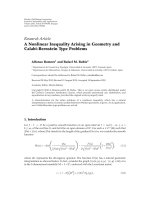
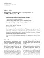
Figure 1: Corrected Dinar acceleration, velocity, and displacement (EW component) using bandpass filter: N = 4, f

p1
= 0.2Hz, f
p2
= 20 Hz.
(vi) significant duration TD: the interval of time over
which a proportion (percentage) of the total I
a
is accu-
mulated (by default: the interval between the 5% and
95% thresholds).
The par ameter t
r
in (2) denotes the total seismic duration, g
is the acceleration of gravity.
3. ANALYSIS OF RESULTS AND CONCLUSIONS
After definition of accelerograms, the corresponding velocity
and displacement time histories are obtained in SeismoSignal
(through single and double time-integration, resp.). We ex-
amine the resulting time histories when the acceleration
Guergana Mollova 5
00.511.522.53
Rp (dB)
1.2
1.4
1.6
1.8
2
2.2
2.4
2.6

2.8
PGA (m/s
2
)
Dinar
Izmit
Kusadasi (
0.1)
(a)
00.51 1.522.53
Rp (dB)
0.2
0.22
0.24
0.26
0.28
0.3
0.32
0.34
0.36
PGV (m/s)
Dinar
Izmit
Kusadasi (
0.01)
(b)
00.511.522.53
Rp (dB)
0.05
0.055

0.06
0.065
0.07
0.075
0.08
0.085
0.09
0.095
0.1
PGD (m)
Dinar
Izmit
Kusadasi (
0.001)
(c)
00.511.522.53
Rp (dB)
0.4
0.6
0.8
1
1.2
1.4
1.6
I
a
(m/s)
Dinar
Izmit
Kusadasi (

0.001)
(d)
00.51 1.522.53
Rp (dB)
0
5
10
15
20
25
30
35
TD (s)
Dinar
Izmit
Kusadasi
(e)
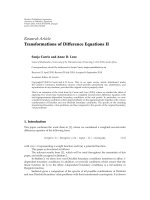
Figure 2: Strong-motion parameters as a function of the passband ripple Rp [dB] (NS component). Note: different scales for Kusadasi
record.
records are bandpass filtered with orders N = 2, 4, 6 (and
N
= 8 for the weakest earthquake with Mw = 3.8). Exam-
ples have shown that only these filters orders could be applied
(under given corner frequency conditions from Ta ble 1). For
higher orders the waveforms of the corrected time histories
are abnormally different compared to the uncorrected ones.
Corrected time series for Dinar station (EW component)
with 4th-order Butterworth, Chebyshev, and Bessel filters
6 EURASIP Journal on Advances in Signal Processing
10 20 30 40

1
2
Frequency (Hz)
Fourier amplitude (m/s)
10
20 30 40
1
2
Frequency (Hz)
Fourier amplitude (m/s)
10 20 3040
1
2
Frequency (Hz)
Fourier amplitude (m/s)
(a) Butterworth
10 20 30 40
1
2
Frequency (Hz)
Fourier amplitude (m/s)
10 20 30 40
1
2
Frequency (Hz)
Fourier amplitude (m/s)
10 20 30 40
1
2
Frequency (Hz)

Fourier amplitude (m/s)
(b) Chebyshev (3 dB)
10 20 30 40
1
2
Frequency (Hz)
Fourier amplitude (m/s)
10 20 30 40
1
2
Frequency (Hz)
Fourier amplitude (m/s)
10 20 30 40
1
2
Frequency (Hz)
Fourier amplitude (m/s)
(c) Bessel
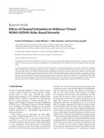
Figure 3: Fourier spectra of acceleration for bandpass filtered Izmit record between 0.12 Hz and 20 Hz for orders N = 2, 4, and 6 (from up
to down) NS component. Note: the graphics in gray color show the uncorrected records.
( f
p1
= 0.2 Hz, f
p2
= 20 Hz) are shown in Figures 1(a), 1(b),
1(c), respectively. It is obvious that in all cases corrected ac-
celeration is affected by the time shift (due to the application
of causal IIR filters).
We have obtained the numerical values of the examined
strong-motion parameters for Butterworth, Chebyshev, or

Bessel processed records using filters from different orders
(not shown here). The only parameter which does not de-
pend on the choice of the filter is TP.
Figure 2 shows the influence of the Chebyshev passband
ripple Rp [dB] on the NS component of Dinar, Izmit, and
Kusadasi records (for N
= 4). Different examinations vary-
ing Rp in the range from 0.2 to 3 dB have been made. The
predominant period TP is a constant value in the above range
and does not depend on Rp. Significant duration TD is al-
most constant too (see the last graphic of Figure 2). However,
the peak values of processed time series and Arias intensity I
a
depend significantly on the variation of Rp (it is valid for al l
station records). We have found that PGA decreases substan-
tially (with up to 15–20%) with increasing Rp. The PGA is
one of the main parameters of interest for engineering appli-
cation. As we have expected, values of all parameters for Rp
=
0.2 dB are the closest to the values obtained with Butterworth
4th-order filter (i.e., maximally flat passband case).
Figure 3 presents the results for FAS of acceleration for
bandpass filtered Izmit record between 0.12 Hz and 20 Hz
for orders N
= 2, 4, and 6 (NS component). The FAS and
the power spectrum (or power spectral densit y function) are
computed in SeismoSignal by means of fast Fourier transfor-
mation (FFT) of the input time history. The Fourier spectra
show how the amplitude of the ground motion is distributed
with respect to frequency (or period), effectively meaning

Guergana Mollova 7
10 20 30 40
0.01
0.02
0.03
Frequency (Hz)
Fourier amplitude (m/s)
10 20 30 40
0.01
0.02
0.03
Frequency (Hz)
Fourier amplitude (m/s)
10 20 30 40
0.01
0.02
0.03
Frequency (Hz)
Fourier amplitude (m/s)
10 20 30 40
0.01
0.02
0.03
Frequency (Hz)
Fourier amplitude (m/s)
(a)
10 20 3040
0.5
1
1.5

Frequency (Hz)
Fourier amplitude (m/s)
10 20 3040
0.5
1
1.5
Frequency (Hz)
Fourier amplitude (m/s)
(b)
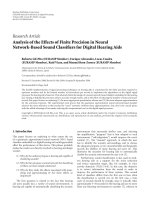
Figure 4: (a) Fourier spectra of acceleration for bandpass Chebyshev filtered Kusadasi record between 3.5 Hz and 18 Hz for N = 4, V
component with Rp
= 0.2 dB and 1.1 dB (left column), and Rp = 2 dB and 3 dB (right column). Note: the graphics in gray color show the
uncorrected records. (b) Fourier spectra of acceleration for bandpass Chebyshev filtered Izmit record between 0.12 Hz and 20 Hz for N
= 4,
V component with Rp
= 1.2 dB (left) and 3 dB (right). Note: the graphics in gray color show the uncorrected records.
that the frequency content of the given accelerogram can be
fully determined.
As explained in [14], a more or less constant amplitude
of the FFT spectrum at frequencies lower than f
p1
or at
frequencies beyond f
p2
is generally an indication of large
low- or high-frequency noise, respectively. We can see in
Figure 3 that the parts of the FAS (uncorrected) below
0.12 Hz and beyond 20 Hz are abnormally high. This proves
the necessit y of application of bandpass filter with the above
frequency edges regarding low-and high-frequency noise

suppression.
Graphical results for FAS confirm that all filter orders ex-
amined could be used except Chebyshev 6th-order filter. As
a best choice we recommend order N = 4 for all stations. Of
course, we should bear in mind the phase distortion caused
by IIR filters. Furthermore, we have proved that the change
of the ripple Rp (Chebyshev filter) has a small influence on
the obtained FAS (Figures 4(a), 4(b)).
8 EURASIP Journal on Advances in Signal Processing
0102030405060
Period (s)
0.03
0.06
0.09
0.12
0.15
0.18
0.21
0.24
0.27
Response displacement (m)
N = 2 (upper plot)
N
= 4(ingraycolor)
N
= 6 (lower plot)
(a)
0 102030405060
Period (s)
0.05

0.1
0.15
0.2
0.25
0.3
0.35
0.4
0.45
Response displacement (m)
N = 2 ( lower plot)
N
= 4(ingraycolor)
N
= 6 (upper plot)
(b)
0 102030405060
Period (s)
0.05
0.1
0.15
0.2
0.25
0.3
0.35
0.4
Response displacement (m)
N = 2 ( upper plot)
N
= 4(ingraycolor)
N

= 6 (lower plot)
(c)
Figure 5: Displacement response spectra for bandpass filtered
Izmit record, NS component, using (a) Butterworth, (b) Chebyshev
(3 dB), (c) Bessel filters.
Finally, the 5%-damped displacement response spectra
(SD) for Izmit record (NS component) have been computed
(Figures 5(a), 5(b)), 5(c), applying different filtering tech-
niques and filter orders. The evaluation is done for periods
between 0.02 second and 60 seconds with a period step of
0.02 second. The graphical results from Figure 5 correspond
to these ones from Figure 3 (Fourier spectra for Izmit record
filtered with the same edge frequencies). As could be seen,
changingthefilterorder(betweentwoandfour/orbetween
two and six) influences the smaller SD. The only exception
is Chebyshev filter with order N
= 6(Figure 5(b)) which re-
flects larger values of SD.
We would like finally to emphasize that all investigations
in this study are carried out using chosen filtering techniques
(Butterworth, Chebyshev-type I, or Bessel methods) and un-
der given parameters (order, edge frequencies, and passband
ripple for Chebyshev filter). The obtained numerical and
graphical results may not be relevant when other filtering
techniques or parameters are applied.
ACKNOWLEDGMENTS
This work is supported by the Alexander von Humboldt
Foundation (Project BUL 1059420). The author would like
also to thank all anonymous reviewers for their useful rec-
ommendations and remarks.

REFERENCES
[1] B. Darragh, W. Silva, and N. Gregor, “Strong motion record
processing for the PEER centre,” in Proceedings of COS-
MOS Invited Workshop on Strong-Motion Record Processing,
Richmond, Calif, USA, May 2004, />recordProcessingPapers.html.
[2] A. F. Shakal, M. J. Huang, and V. M. Graizer, “CSMIP
strong-motion data processing,” in Proceedings of COSMOS
Invited Workshop on Strong-Motion Record Processing, Rich-
mond, Calif, USA, May 2004, />recordProcessingPapers.html.
[3] D. Rinaldis, “Aquisition and processing of analogue and dig-
ital accelerometric records: ENEA methodology and experi-
ence from Italian earthquakes,” in Proceedings of COSMOS
Invited Workshop on Strong-Motion Record Processing, Rich-
mond, Calif, USA, May 2004, />recordProcessingPapers.html.
[4] “Internet Site of the European Strong-Motion Database,”
.
[5]D.M.BooreandS.Akkar,“Effect of causal and acausal fil-
ters on elastic and inelastic response spectra,” Ear thquake En-
gineering and Str uctural Dynamics, vol. 32, no. 11, pp. 1729–
1748, 2003.
[6] D. M. Boore, “On pads and filters: processing strong-motion
data,” Bulletin of the Seismological Society of America, vol. 95,
no. 2, pp. 745–750, 2005.
[7] D. M. Boore and J. J. Bommer, “Processing of strong-motion
accelerograms: needs, options and consequences,” Soil Dy-
namics and Earthquake Engineering, vol. 25, no. 2, pp. 93–115,
2005.
Guergana Mollova 9
[8] P. Bazzurro, B. Sjoberg, N. Luco, W. Silva, and R. Darragh,
“Effects of strong motion processing procedures on time his-

tories, elastic and inelastic spectra,” in Proceedings of COS-
MOS Invited Workshop on Strong-Motion Record Processing,
Richmond, Calif, USA, May 2004, />recordProcessingPapers.html.
[9] A.Pazos,M.J.Gonz
´
alez, and G. Alguacil, “Non-linear filter,
using the wavelet transform, applied to seismological records,”
Journal of Seismology, vol. 7, no. 4, pp. 413–429, 2003.
[10] F. Scherbaum, Of Poles and Zeros: Fundamentals of Digital
Seismology, Kluwer Academic, Dordrecht, The Netherlands,
2nd edition, 2000.
[11] “SeismoSignal - a computer program for signal processing
of strong-motion data,” 2004, ver.3.1.0, smosoft
.com.
[12] A. Plesinger, M. Zmeskal, and J. Zednik, Automated Preprocess-
ing of Digital Seismograms - Principles and Software,Prague-
Golden, Prague, Czech Republic, 1996.
[13] A. M. Converse and A. G. Brady, “BAP: basic strong-motion
accelerogram processing software; ver.1.0,” Open-File Report
92-296A, p. 178, U.S. Geological Survey, Denver, Colo, USA,
1992.
[14] M. Zar
´
e and P Y. Bard, “Strong motion dataset of Turkey: data
processing and site classification,” Soil Dynamics and Earth-
quake Engineering, vol. 22, no. 8, pp. 703–718, 2002.
[15] D. Rinaldis, J. M. H. Menu, and X. Goula, “A study of vari-
ous uncorrected versions of the same ground acceleration sig-
nal,” in Proceedings of the 8th European Conference on Earth-
quake Eng ineering (ECEE ’86), vol. 7, pp. 1–8, Lisbon, Portu-

gal, September 1986.
[16] D. M. Boore, “Effect of baseline corrections on displacements
and response sp ectra for several recordings of the 1999 Chi-
Chi, Taiwan, earthquake,” Bulletin of the Seismolog ical Society
of America, vol. 91, no. 5, pp. 1199–1211, 2001.
Guergana Mollova received the M.S. and
Ph.D. degrees both in electronics from
the Technical University of Sofia, Bulgaria.
Since 1992, she i s with the Department of
Computer-Aided Engineering of the Uni-
versity of Architecture, Civil Engineering
and Geodesy of Sofia, where she is currently
an Associate Professor. Her main research
area is digital signal processing theory and
methods, including the least-squares ap-
proach for one- and multidimensional digital filters, digital dif-
ferentiators, and Hilbert transformers. During the last years her
research interests are focused on application aspects of digital fil-
tering techniques for analysis of data records from strong-motion
earthquakes. She is Senior Member of IEEE and also Member of
several national professional organizations. She is a recipient of the
Alexander von Humboldt Foundation Fellowship.