Báo cáo hóa học: " Research Article A Review of Signal Subspace Speech Enhancement and Its Application to Noise Robust Speech Recognition potx

Hindawi Publishing Corporation
EURASIP Journal on Advances in Signal Processing
Volume 2007, Article ID 45821, 15 pages
doi:10.1155/2007/45821
Research Article
A Review of Signal Subspace Speech Enhancement and
Its Application to Noise Robust Speech Recognition
Kris Hermus, Patrick Wambacq, and Hugo Van hamme
Department of Electrical Engineering - ESAT, Katholieke Universiteit Leuven, 3001 Leuven-Hever lee, Belgium
Received 24 October 2005; Revised 7 March 2006; Accepted 30 April 2006
Recommended by Kostas Berberidis
The objective of this paper is threefold: (1) to provide an extensive review of signal subspace speech enhancement, (2) to derive
an upper bound for the performance of these techniques, and (3) to present a comprehensive study of the potential of subspace
filtering to increase the robustness of automatic speech recognisers against stationary additive noise distortions. Subspace filtering
methods are based on the orthogonal decomposition of the noisy speech observation space into a signal subspace and a noise
subspace. This decomposition is possible under the assumption of a low-rank model for speech, and on the availability of an
estimate of the noise correlation matrix. We present an extensive overview of the available estimators, and derive a theoretical
estimator to experimentally assess an upper bound to the performance that can be achieved by any subspace-based method.
Automatic speech recognition (ASR) experiments with noisy data demonstrate that subspace-based speech enhancement can
significantly increase the robustness of these systems in additive coloured noise environments. Optimal performance is obtained
only if no explicit rank reduction of the noisy Hankel matrix is performed. Although this strategy might increase the level of the
residual noise, it reduces the r i sk of removing essential signal information for the recogniser’s back end. Finally, it is also shown
that subspace filtering compares favourably to the well-known spectral subtraction technique.
Copyright © 2007 Kris Hermus et al. This is an open access article distributed under the Creative Commons Attribution License,
which permits unrestricted use, distribution, and reproduction in any medium, provided the or iginal work is properly cited.
1. INTRODUCTION
One particular class of speech enhancement techniques that
has gained a lot of attention is signal subspace filtering. In
this approach, a nonparametric linear estimate of the un-
known clean-speech signal is obtained based on a decom-
position of the observed noisy signal into mutually orthog-

onal sig nal and noise subspaces. This decomposition is pos-
sible under the assumption of a low-rank linear model for
speech and an uncorrelated additive (white) noise interfer-
ence. Under these conditions, the energy of less correlated
noise spreads over the whole observation space while the en-
ergy of the correlated speech components is concentrated in a
subspace thereof. Also, the signal subspace can be recovered
consistently from the noisy data. Generally speaking, noise
reduction is obtained by nulling the noise subspace and by re-
moving the noise contribution in the signal subspace.
The idea to perform subspace-based signal estimation
was originally proposed by Tufts et al. [1]. In their work,
the signal estimation is actually based on a modified SVD
of data matrices. Later on, Cadzow [2] presented a general
framework for recovering signals from noisy observations. It
is assumed that the original signal exhibits some well-defined
properties or obeys a certain model. Signal enhancement is
then obtained by mapping the observed signal onto the space
of signals that possess the same structure as the clean signal.
This theory forms the basis for all subspace-based noise re-
duction algorithms.
A first and indispensable step towards noise reduction
is obtained by nulling the noise subspace (least squares
(LS) estimator) [3]. However , for improved noise reduction,
also the noise contribution in the (signal + noise) subspace
should be suppressed or controlled, which is achieved by all
other estimators as is explained in subsequent sections of this
paper.
Of particular interest is the minimum variance (MV) es-
timation, which gives the best linear estimate of the clean

data, given the rank p of the clean signal and the variance of
the white noise [4, 5]. Later on, a subspace-based speech en-
hancement with noise shaping was proposed in [6]. Based on
the observation that signal distortion a nd residual noise can-
not be minimised simultaneously, two new linear estimators
2 EURASIP Journal on Advances in Signal Processing
are designed—time domain constrained (TDC) and spectral
domain constrained (SDC)—that keep the level of the resid-
ual noise below a chosen threshold while minimising signal
distortion. Parameters of the algorithm control the trade-off
between residual noise and signal distortion. In subspace-
based speech enhancement with true perceptual noise shap-
ing, the residual noise is shaped according to an estimate of
the clean signal masking threshold, as discussed in more re-
cent papers [7–9].
Although basic subspace-based speech enhancement is
developed for dealing with white noise distortions, it can eas-
ily be extended to remove general coloured noise provided
that the noise covariance matrix is known (or can be esti-
mated) [10, 11]. A detailed theoretical analysis of the un-
derlying pr inciples of subspace filtering can, for example, be
found in [4, 6, 12].
The excellent noise reduction capabilities of subspace fil-
tering techniques are confirmed by several studies, both with
the basic LS estimate [3] and with the more advanced optimi-
sation criteria [6, 10, 13]. Especially for the MV and SDC es-
timators, a speech quality improvement that outperforms the
spectral subtraction approach is revealed by listening tests.
Noise suppression facilitates the understanding, commu-
nication, and processing of speech signals. As such, it also

plays an important role in automatic speech recognition
(ASR) to improve the robustness in noisy environments. The
latter is achieved by enhancing the observed noisy speech sig-
nal prior to the recogniser’s preprocessing and decoding op-
erations. In ASR applications, the effectiveness of any speech
enhancement algorithm is quantified by its potential to close
the gap between noisy and clean-speech recognition accu-
racy.
Opposite to what happens in speech communication ap-
plications, the improvement in intelligibility of the speech
and the reduction of listener’s fatigue are of no concern. Nev-
ertheless, a correlation can be expected between the improve-
ments in perceived speech quality on the one hand, and the
improvement in recognition accuracy on the other hand.
Ver y few papers discuss the application of signal sub-
space methods to robust speech recognition. In [14]an
energy-constrained signal subspace (ECSS) method is pro-
posed based on the MV estimator. For the recognition of
large-vocabulary continuous speech (LV-CS) corrupted by
additive white noise, a relative reduction in WER of 70%
is reported. In [15], MV subspace filtering is applied on a
LV-CS recognition (LV-CSR) task distorted with white and
coloured noise. Significant WER reductions that outperform
spectral subtraction are reported.
Paper outline
In this paper we elaborate on previous paper [16]and
describe the potential of subspace-based speech enhance-
ment to improve the performance of ASR in noisy condi-
tions. At first, we extensively review several subspace esti-
mation techniques and classify these techniques based on

the optimisation criteria. Next, we conduct a performance
comparison for both white and coloured noise removal from
a speech enhancement and especially from a speech recog-
nition perspective. The impact of some crucial parame-
ters, such as the analysis window length, the Hankel matrix
dimensions, the signal subspace dimension, and method-
specific design parameters will be discussed.
2. SUBSPACE FILTERING
2.1. Fundamentals
Any noise reduction technique requires assumptions about
the nature of the interfering noise signal. Subspace-based
speech enhancement also makes some basic assumptions
about the properties of the desired signal (clean speech) as
is the case in many—but not all—signal enhancement algo-
rithms. Evidently, the separation of the speech and noise sig-
nals wil l be based on their different characteristics.
Since the characteristics of the speech (and also of the
noise) signal(s) are time varying, the speech enhancement
procedure is performed on overlapping analysis frames.
Speech signal
A key assumption in all subspace-based signal enhance-
ment algorithms is that every short-time speech vector s
=
[s(1), s(2), , s(q)]
T
can be written as a linear combination
of p<qlinearly independent basis functions m
i
, i = 1, , p,
s

= My (1)
where M is a (q
× p) matrix containing the basis functions
(column-wise ordered) and y is a length-p column vector
containing the weights. Both the number and the form of
these basis functions will in general be time varying (frame-
dependent).
An obvious choice for m
i
are (damped) sinusoids mo-
tivated by the traditional sinusoidal model (SM) for speech
signals. A crucial observ ation here is that the consecut ive
speech vectors s will occupy a (p<q)-dimensional subspace
of t he q-dimensional Euclidean space (p equals the signal or-
der). Because of the time-varying nature of speech signals,
the location of this signal subspace (and its dimension) will
consequently be frame-dependent.
Noise signal
The additive noise is assumed to be zero-mean, white, and
uncorrelated with the speech signal. Its variance should be
slowly time varying such that it can be estimated from noise-
only segments. Contrarily to the speech signal, consecutive
noise vectors n will occupy the whole q-dimensional space.
Speech/noise separation
Based on the above description of the speech and noise sig-
nals, the aforementioned q-dimensional observation space
is split in two subspaces, namely a p-dimensional (signal +
noise) subspace in which the noise interferes with the speech
signal, and a (q
− p)-dimensional subspace that contains only

Kris Hermus et al. 3
noise (and no speech). The speech enhancement procedure
can now be summarised as fol lows:
(1) separate the (sig nal+noise) subspaces f rom the (noise-
only) subspace,
(2) remove the (noise-only) subspace,
(3) optionally, remove the noise components in the (signal
+ noise) subspace.
1
The first operation is straightforward for the white noise
condition under consideration here, but can become com-
plicated for the coloured noise case as we will see further on.
The second operation is applied in all implementations of
subspace-based signal enhancements, whereas the third op-
eration is indisp ensable to obtain an increased noise reduc-
tion. Nevertheless, the last operation is sometimes omitted
because of the introduction of speech distortion. The latter
problem is inevitable since the speech and noise signals over-
lap in the signal subspace.
In the next section we will explain that the orthogonal
decomposition into frame-dependent signal and noise sub-
spaces can be performed by an SVD of the noisy signal ob-
servation matrix, or equivalently by an eigenvalue decompo-
sition (EVD) of the noisy signal correlation matrix.
2.2. Algorithm
Let s(k) represent the clean-speech samples and let n(k)be
the zero-mean, additive white noise distortion that is as-
sumed to be uncorrelated with the clean speech. The ob-
served noisy speech x(k) is then given by
x( k)

= s(k)+n(k). (2)
Further, let
¯
R
x
,
¯
R
s
,and
¯
R
n
be (q × q)(withq>p)trueauto-
correlation matrices of x(k), s(k), and n(k), respectively. Due
to the assumption of uncorrelated speech and noise, it is clear
that
¯
R
x
=
¯
R
s
+
¯
R
n
. (3)
The EVD of

¯
R
s
,
¯
R
n
,and
¯
R
x
can be written as follows:
¯
R
s
=
¯
V
¯
Λ
¯
V
T
,(4)
¯
R
n
=
¯
V


σ
2
w
I

¯
V
T
,(5)
¯
R
x
=
¯
V

¯
Λ + σ
2
w
I

¯
V
T
,(6)
with
¯
Λ a diagonal matrix containing the eigenvalues

¯
λ
i
,
¯
V an
orthonor m al matrix containing the eigenvectors
¯
v
i
, σ
2
w
the
noise variance, and I the identity matrix. A crucial observa-
tion here is that the eigenvectors of the noise are identical to
the clean-speech eigenvectors due to the white noise assump-
tion such that the eigenvectors of
¯
R
s
can be found from the
EVD of
¯
R
x
in (6).
1
For brevity, the (signal + noise) subspace will further be called the sig nal
subspace, and the (noise-only) subspace will be referred to as the noise

subspace.
Based on the assumption that the clean speech is con-
fined to a (p<q)-dimensional subspace (1), we know that
¯
R
s
has only p nonzero eigenvalues
¯
λ
i
.If
¯
λ
i
>σ
2
w
(i = 1, , p), (7)
the noise can be separated from the speech signal, and the
EVD of
¯
R
x
can be rewritten as
¯
R
x
=

¯

V
p
¯
V
q−p


¯
Λ
p
0
00

+ σ
2
w

I
p
0
0 I
q−p


¯
V
p
¯
V
q−p


T

(8)
if we assume that the elements
¯
λ
i
of
¯
Λ are in descending or-
der. The subscripts p and q
− p refer to the signal and noise
subspaces, respectively.
Regardless of the specific optimisation criterion, speech
enhancement is now obtained by
(1) restricting the enhanced speech to occupy solely the
signal subspace by nulling its components in the noise
subspace,
(2) changing (i.e., lowering) the eigenvalues that corre-
spond to the signal subspace.
Mathematically this enhancement procedure can be writ-
ten as a filtering operation on the noisy speech vector x
=
[x(1), x(2), , x(q)]
T
:
s = Fx (9)
with the filter matrix F given by
F

=
¯
V
p
G
p
¯
V
T
p
(10)
in which the (p
× p) diagonal matrix G
p
contains the weight-
ing factors g
i
for the first p eigenvalues of
¯
R
x
, while
¯
V
T
and
¯
V are known as the KLT (Karhunen Loeve transform) ma-
trix and its inverse, respectively. T he filter matrix F can be
rewritten as

F
=
p

i=1
g
i
¯
v
i
¯
v
T
i
, (11)
which illustrates that the filtered signal can be seen as the sum
of p outputs of a “filter bank” (see below). Each filter in this
filter bank is solely dependent on one eigenvector
¯
v
i
and its
corresponding gain factor g
i
.
From EVD to SVD filtering
In many implementations the true covariance matrices in (4)
to (6)areestimatedasR
x
= H

T
x
H
x
,withH
x
(= H
s
+ H
n
)an
(m
× q)(withm>q) noisy Hankel (or Toeplitz)
2
signal ob-
servation matr ix constructed from a noisy speech vector x
2
Because of the equivalence of the Hankel and Toeplitz matrices, that is, a
Toeplitz matrix can be converted into a Hankel matrix by a simple permu-
tation of its rows, any further derivation and discussion will be restricted
to Hankel matrices only.
4 EURASIP Journal on Advances in Signal Processing
x(k)
v
1
v
2
v
p
.

.
.
Jv
1
Jv
2
Jv
p
.
.
.
g
1
g
2
g
p
.
.
.
Σ
D
s(k)
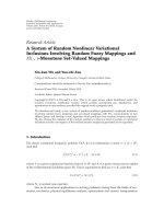
Figure 1: FIR-filter implementation of subspace-based speech en-
hancement. Each singular triplet corresponds to a zero-phase fil-
tered version of the noisy signal.
containing N (N  q,andm + q = N +1)samplesofx(k).
In that case an equivalent speech enhancement can be ob-
tained via the SVD of H
x

[6]. A commonly used modified
SVD-based speech enhancement procedure proceeds as fol-
lows.
Let the SVD of H
x
be given by
H
x
= UΣV
T
. (12)
If the short-time speech and noise sig nals are orthogonal
(H
T
s
H
n
= 0) and if the short-time noise signal is white
(H
T
n
H
n
= σ
2
ν
I), then
H
x
= U



¯
Σ
2
+ σ
2
ν
I

V
T
(13)
with
¯
Σ the matrix containing the singular values of the clean
Hankel mat rix H
s
,andσ
ν
the 2-norm of the columns of H
n
(observe that for large N and in the case of stationary white
noise, σ
2
ν
/m converges in the mean square sense to σ
2
w
).

Under weak conditions, the empirical covariance matrix
H
T
x
H
x
/N will converge to the true autocorrelation matrix
¯
R
x
.
In other words, for sufficiently large N, the subspace that is
spanned by the p dominant eigenvectors of V will converge
to the subspace that is spanned by the vectors of
¯
V
p
from (6).
The enhanced matrix

H
s
is then obtained as

H
s
= U
p
G
p

Σ
p
V
T
p
(14)
or

H
s
=
p

i=1
g
i
σ
i
u
i
v
T
i
(15)
with σ
i
denoting the ith singular value of Σ.
The enhanced signal
s(k) is recovered by averaging along
the antidiagonals of


H
s
. Dologlou and Carayannis [17], and
later on Hansen and Jensen [18] proved that this over-
all procedure is equivalent to one global FIR-filtering op-
eration on the noisy time signal (Figure 1). Each filter
bank output g
i
σ
i
u
i
v
T
i
is obtained by filtering the noisy sig-
nal x(k) with its corresponding eigenfilter v
i
and its re-
versed version Jv
i
. From filter theory we know that this
results in a zero-phase filtering operation. The extraction
of the enhanced signal
s(k) from the enhanced observa-
tion matrix

H
s

is equivalent to a multiplication of

H
s
by the diagonal matrix D (see Figure 1). The elements
{1, 1/2, 1/3, ,1/q,1/q, ,1/q, ,1/3, 1/2, 1} on the diag-
onal of D account for the difference in length of the antidiag-
onals of the signal observation matrix.
This FIR-filter equivalence is an important finding and
gives an interesting frequency-domain interpretation of the
signal subspace denoising operation.
The main advantage of working with the SVD, instead
of the EVD, is that no explicit estimation of the covariance
matrix is needed. In this paper we will further focus on the
SVD description. However, it is stressed that all estimators
can as well be performed in an EVD-based scheme, which
allows for the use of any arbitrary (structured) covariance
estimates like, for example, the empirical Toeplitz covariance
matrix.
2.3. Optimisation criteria
By applying a specific estimation criterion, the elements of
the weighting matrix G
p
from (14) can be found. In this sec-
tion the most common of these criteria are briefly reviewed.
Note that the derivations and statements below are only exact
if the aforementioned conditions (speech of order p,white
noise interference, and orthogonality of speech and noise)
are fulfilled.
Least squares

The least squares (LS) estimate

H
LS
is defined as the best
rank-p approximation of H
x
:
min
rk(

H
LS
)=p


H
x
−

H
LS


2
F
(16)
with rk(A)and
A
2

F
denoting the rank and the Frobenius of
matrix A,respectively.
The LS estimate is obtained by tr uncating the SVD
UΣV
T
of H
x
to rank p:

H
LS
= U
p
Σ
p
V
T
p
. (17)
Observe that this estimate removes the noise subspace, but
keeps the noisy signal unaltered in the signal subspace. This
estimate yields an enhanced signal with the highest residual
noise level (
= (p/q)σ
2
ν
) but with the lowest signal distortion
(
= 0). The performance of the LS estimator is crucially de-

pendent on the estimation of the signal rank p.
Minimum variance
Given the rank p of the clean speech, the MV estimate

H
MV
is the best approximation of the original matrix H
s
that can
be obtained by making linear combinations of the columns
of H
x
:

H
MV
= H
x
T (18)
with
T
= arg min
T∈R
q×q


H
x
T − H
s



2
F
. (19)
Kris Hermus et al. 5
In algebraic terms,

H
MV
is the geometric projection of H
s
onto the column space of H
x
, and is obtained by setting
g
MV,i
= 1 −
σ
2
ν
σ
2
i
. (20)
The MV estimate is the linear estimator with the lowest resid-
ual noise level (LMMSE estimator) [4, 5], and is related to
Wiener filtering and spectral subt raction.
Singular value adaptation
In the singular value adaptation (SVA) method [5], the p

dominant singular values of H
x
are mapped onto the orig-
inal (clean) singular values of H
s
by setting
g
SVA,i
=

σ
2
i
− σ
2
ν
σ
i
. (21)
Observe that
g
SVA,i
=

g
MV,i
(22)
which illustrates the conservative noise reduction of the SVA
estimator.
Time domain constrained

The TDC estimate is found by minimising the signal distor-
tion while setting a user-defined upper bound on the resid-
ual noise level via a control parameter μ
≥ 0. In the modified
SVD of H
x
, g
TDC,i
is given by
g
TDC,i
=
1 − σ
2
ν
/σ
2
i
1 −

σ
2
ν
/σ
2
i

(1 − μ)
. (23)
This estimator can be seen as a Wiener filter with adjustable

input noise level μσ
2
ν
[6].
If μ
= 0, the gains for the signal subspace components are
all set to one which means that the TDC estimator becomes
equal to the LS estimator. Also, the MV estimator is a special
case of TDC with μ
= 1.
The most straig htforward way to specify the value of μ is
to assign a constant value to it, independently of the speech
frameathand.Amorecomplexmethodistoletμ depend on
the SNR of the actual fr ame [19]. Typically μ ranges from 2
to 3.
Spectral domain constrained
A simple form of residual noise shaping is provided by the
SDC estimator. Here, the estimate is found by minimising
the signal distortion subject to constraints on the energy of
the projections of the residual noise onto the signal subspace.
More than one solution for the gain factors in the modified
SVD exists. One possible expression for g
SDC,i
is [6]
g
SDC 1,i
=




exp

−
βσ
2
ν
σ
2
i
− σ
2
ν

(24)
with β
≥ 0, but mostly ≥ 1forsufficient noise reduction. We
will further refer to this estimator as SDC
1. An alternative
solution [6] is to choose
g
SDC 2,i
=

1 −
σ
2
ν
σ
2
i


γ/2
(25)
with γ
≥ 1, further denoted as SDC 2. The amount of noise
reduction can be controlled by the parameters β and γ.Note
that the SDC
2 estimator is a generalisation of both the MV
estimator (20)forγ
= 2 and the SVA estimator (21)forγ =
1.
Extensions of the SDC estimator that exploit the infor-
mation obtained from a perceptual model have been pre-
sented [7, 8].
Optimal estimator
In practice, the assumption of a low-rank speech model (1)
will almost never be (exactly) met. Also, the processing of
short frames will cause deviations from assumed properties
such as orthogonality of speech and noise (finite sample be-
haviour). Consequently, the eigenvectors of the noisy speech
are not identical to the clean-speech eigenvectors such that
the signal subspace will not be exactly recovered ((6)isnot
valid). Also, the measurement of the perturbation of the sin-
gular values of H
s
as stated in (13) will not be exact (the sin-
gular value spectrum of the noise Hankel matr ix H
n
will not
be isotropic if H

T
n
H
n
= kI). In particular, the empirical cor-
relation estimates will not yield a diagonal covariance matrix
for the noise, and the assumption of independence of speech
and noise will mostly not be true for short-time segments. As
a result, the noise reduction that is obtained with the above
estimators will not be optimal.
It is interesting to quantify the decrease in performance
in such situations. Thereto we derive our so-called optimal
estimator (OPT).
Assume that both the clean and noisy observation matri-
ces H
s
and H
x
are observable (= cheating experiment). We
will now explain how to find the optimal-in LS sense-gain
factors g
OPT,i
[20]. If the SVD of H
x
is given by
H
x
= UΣV
T
, (26)

the optimal estimate

H
OPT
of H
s
is defined as
H
OPT
= arg min
G
p


U
p
Σ
p
G
p
V
T
p
− H
s


2
F
, (27)

where, again, the subscript p denotes truncation to the p
largest singular vectors/values (of H
x
).
In other words, based on the exact knowledge of H
s
,we
modify the singular values of H
x
such that H
OPT
is closest to
H
s
in LS sense.
Based on the dyadic decomposition of the SVD, it can be
shown that the optimal gains g
OPT,i
(i = 1, , p)aregiven
by the following expression:
G
p,OPT
= diag

U
T
p
H
s
V

p

Σ
−1
p
(28)
where diag
{A} is a diagonal matrix constructed from the el-
ements on the diagonal of matrix A.
6 EURASIP Journal on Advances in Signal Processing
Proof. The values g
OPT,i
(i = 1, , p) are found by minimis-
ing the following cost function that is equivalent to (27):
C

g
1
, , g
p

=
m

k=1
q

l=1

H

s
(k, l) −
p

j=1
g
j
H
x, j
(k, l)

2
(29)
where A(k, l) is the element on row k and column l of matrix
A,andH
x, j
= σ
j
u
j
v
T
j
is the jth rank-one matrix in the dyadic
decomposition of H
x
.
Taking the derivative of C with respect to g
i
and setting

to zero yield:
∂C
∂g
i
= 2
m

k=1
q

l=1

H
s
(k, l) −
p

j=1
g
j
H
x, j
(k, l)

H
x,i
(k, l)

=
0.

(30)
Since u
T
i
v
j
= δ
i, j
and v
T
i
v
j
= δ
i, j
,weget
g
OPT,i
=
u
T
i
H
s
v
i
σ
i
. (31)
Note that in the derivation of the optimal estimator we do

not take into account the averaging along the antidiagonals to
extract the enhanced signal. However, the latter operation is
not necessarily needed to obtain an optimal result [21].
Also, it can be proven that g
i,OPT
= g
i,MV
if the assump-
tions of orthogonality and white noise are fulfilled [20].
2.4. Visualisation of the gain factors
An interesting comparison between the different estimators
is obtained by plotting the gain factors g
i
as a function of the
unbiased spec tral SNR :
SNR
spec,unbiased
= 10 log
10
¯
σ
2
i
σ
2
ν
. (32)
By rewriting the expressions for g
i
as a function of a

def
=
¯
σ
2
i
/σ
2
ν
,
we get
g
LS,i
= 1, g
MV,i
=
a
1+a
,
g
SVA,i
=

a
1+a

1/2
, g
TDC,i
=

a
μ + a
,
g
SDC 1,i
= exp

−
β
2a

, g
SDC 2,i
=

a
1+a

γ/2
.
(33)
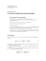
In Figure 2 these gains are plotted as a function of the un-
biased spectral SNR. Evidently, for all estimators, g
i
ranges
from 0 (low spectral SNR, only noise) to 1 (high spectral
SNR, noise free).
In practice, some of the estimators require flooring in
order to avoid negative values for the weights g
i

. Indeed, in
these estimators the singular values
¯
σ
i
of the clean-speech
matrix are implicitly estimated as σ
2
i
− σ
2
ν
. Evidently, the lat-
ter expression can become negative, especially in very noisy
conditions. Negative weights become apparent when the gain
factors are expressed (and visualised) as a function of the bi-
ased spec tral SNR
spec,biased
= 10 log
10
(σ
2
i
/σ
2
ν
).
2.5. Relation to spectral subtraction
and Wiener filtering
From the above discussion the strong similarity between

subspace-based speech enhancement and spectral subtrac-
tion should have become clear [6]. While spectral subtrac-
tion is based on a fixed FFT, the SVD-based method relies
on a data-dependent KLT,
3
which results in larger compu-
tational load. For a frame of N samples, the FFT requires
(N/2)
· log
2
(N) operations, whereas the complexity of the
SVD of a matrix with dimensions m
× q is given by O(mq
2
).
Recall that m
 q,withq typically between 8 and 20, and
with m + q
− 1 = N. This means that for typical values of N
and q,theSVDrequires10upto100timesmorecompu-
tations than the FFT. However, real-time implementations
of subspace speech enhancement are feasible on nowadays
(high-end) hardware.
Another major difference between subspace-based
speech enhancement and spectral subtraction is the explicit
assumption of signal order or, equivalently, a rank-deficient
speech observation matrix or a rank-deficient speech cor-
relation matrix. Note that in Wiener filtering, this rank
reduction is done implicitly by the estimation of a (possibly)
rank-reduced speech correlation matrix.

For completeness we mention that beside FFT-based
and SVD-based speech enhancement, also a DCT-based en-
hancement approach is possible [22]. While the DCT pro-
vides a better energy compaction than the FFT, it is still in-
ferior to the theoretically optimal KLT transform that is used
in subspace filtering.
3. IMPLEMENTATION ASPECTS
In this section we discuss the choice of the most impor-
tant parameters in the SVD-based noise reduction algorithm,
namely the frame length N, the dimensions of H
x
, and the
dimension p of the signal subspace.
3.1. Signal subspace dimension
In theory the dimension of the signal subspace is defined by
the order of the linear signal model in (1). However, in prac-
tice the speech contents will strongly vary (e.g., voiced versus
unvoiced segments) and the entire signal will never exactly
obey one model. Several techniques, such as minimum de-
scription length (MDL) [23] were developed to estimate the
model order. Sometimes, the order p is chosen on a frame-
by-frame basis, and, for example, chosen as the number of
positive eigenvalues of the estimate R
s
of
¯
R
s
. A rather similar
strategy is to set p such that the energy of the enhanced sig-

nal is as close as possible to an estimate of the clean-speech
energy. This concept was introduced in [24] and is called
3
The FFT and KLT coincide if the signal observation matrix is circulant.
Kris Hermus et al. 7
30 20 100 102030
0
0.2
0.4
0.6
0.8
1
Spectral SNR (dB)
Gain factor g
i
μ = 1(= MV)
μ
= 3
μ
= 5
(a) TDC
30 20 100 102030
0
0.2
0.4
0.6
0.8
1
Spectral SNR (dB)
Gain factor g

i
β = 1
β
= 3
β
= 5
β
= 7
(b) SDC 1
30 20 100 102030
0
0.2
0.4
0.6
0.8
1
Spectral SNR (dB)
Gain factor g
i
γ = 1(= SVA)
γ
= 2(= MV)
γ
= 4
γ
= 6
(c) SDC 2
30 20 100 102030
0
0.2

0.4
0.6
0.8
1
Spectral SNR (dB)
Gain factor g
i
SVA
MV
SDC
1(β = 2)
(d) MV / SVA / SDC 1
Figure 2: Gain factors for the different estimators as a function of the spectral SNR.
“parsimonious order”. For 16 kHz data the value of p is usu-
ally around 12.
3.2. Frame length
The frame length N must be larger than the order of the as-
sumed signal model, such that the correlation that is embed-
ded in the speech signal can be fully exploited to split the lat-
ter signal from the noise. On the other hand, the frame length
is limited by the time over which the speech and noise can be
assumed stationary (usually 20 to 30 milliseconds). Besides,
N must not be too large to avoid prohibitively large compu-
tations in the SVD of H
x
. Hence, the value of N is typically
between 320 and 480 samples for 16 kHz data.
3.3. Matrix dimension
Observe that the dimensions (m
× q)ofH

x
cannot be chosen
independently due to the relation m +q
= N + 1. The smaller
dimension q of H
x
should be larger than the order of the as-
sumed signal model, such that the separation into a signal
and a noise subspace is possible. If q is small, for example,
q
≈ p, the smallest nont rivial singular value of H
s
decreases
strongly and becomes of the same magnitude as the largest
singular value of the noise, such that the determination of
the signal subspace becomes less accurate. For this reason, q
must not be taken too small [5].
Asufficiently high value for m is beneficial for the noise
removal, since the necessary conditions of orthogonality of
speech and noise (i.e., H
T
s
H
n
= 0), and white noise (H
T
n
H
n
=

σ
2
ν
I) will on average be better fulfilled. Also, for large m, the
noise threshold that a dds up to every singular value of H
s
(see (13)) becomes more and more pronounced such that the
expressions for the gain functions g
i
become more accurate.
Note that the value of m is bounded since the value of q de-
creases for increasing values of m. A good compromise is to
choose m intherange20to30(16kHzdata).
For more information on the choice of m and q we refer
to [4, 5].
4. EXTENSION TO COLOURED NOISE
If the additive noise is not white, the noise correlation ma-
trix
¯
R
n
cannot be diagonalised by the matrix
¯
V with the right
8 EURASIP Journal on Advances in Signal Processing
eigenvectors of H
s
, and the expressions for the EVD of
¯
R

x
(6)
and SVD of H
x
(13) are no longer valid. In this case, a differ-
ent procedure should be applied. It is assumed that the noise
statistics have been estimated during noise-only segments, or
even during speech activity itself [25–27]. Below, we shortly
review the most common extensions of the basic subspace
filtering theory to coloured noise conditions.
4.1. Explicit pre- and dewhitening
ThemodifiedSVDnoisereductionschemecaneasilybeex-
tended to the general coloured noise case if the Cholesky fac-
tor R of the noise signal is known or has been estimated.
4
Indeed, the noise can be prewhitened by a multiplication by
R
−1
[4, 5]:
H
x
R
−1
=

H
s
+ H
n


R
−1
(34)
such that

H
n
R
−1

T

H
n
R
−1

=
Q
T
Q = I. (35)
A corresponding dewhitening operation (a postmultiplica-
tion by the matrix R) should be included after the SVD mod-
ification.
4.2. Implicit pre- and dewhitening
Because subsequent pre- and dewhitening can cause a loss of
accuracy due to numerical instability, usually an implicit pre-
and dewhitening is p erformed by working with the quotient
SVD (QSVD)
5

of the matrix pair (H
x
, H
n
)[10]. The QSVD
of (H
x
, H
n
)isgivenby
H
x
=

UΔΘ
T
,
H
n
=

VMΘ
T
.
(36)
In this decomposition,

U and

V are unitary matr ices, Δ and

M are diagonal matrices with δ
1
≥ δ
2
≥···≥δ
q
and μ
1
≤
μ
2
≤··· ≤ μ
q
,andΘ is a nonsingular (invertible) matrix.
Including the truncation to rank p, the enhanced matrix
is now given by [10]:

H
s
=

U
p

Δ
p
G
p

Θ

T
p
. (37)
The expressions for G
p
are the same as for the white noise
case, but considering that σ
2
ν
is now equal to 1 due to the
prewhitening. Also, the QSVD-based noise reduction can be
interpreted as a FIR-filtering operation, in a way that is very
similar to the white noise case [18].
A QSVD-based prewhitening scheme for the reduction
of rank-deficient noise has recently been proposed by Hansen
and Jensen [29].
4
Note that R can be obtained either via the QR-factorisation of the noise
Hankel matrix H
n
= QR, or via the Cholesky decomposition of the noise
correlation matrix R
n
= R
T
R.
5
Originally called the generalised SVD in [28].
Optimal estimator
The generalisation of the optimal estimator (OPT) in (28)to

the coloured noise case is rather straightforward. The expres-
sion for the QSVD implementation is found by

H
OPT
= arg min
G
p



U
p
Δ
p
G
p
Θ
T
p
− H
s


2
F
(38)
which leads to [20]
G
p,OPT

= diag


U
T
p
H
s
Θ
T
p

diag

Θ
T
p
Θ
p

−1
Δ
−1
p
. (39)
This expression is very similar to the white noise case (28),
except for the inclusion of a normalisation step. The latter
is necessary since the columns of the matrix Θ are not nor-
malised.
4.3. Signal/noise KLT

A major drawback of pre- and dewhitening is that not only
the additive noise but also the original signal is affected by
the transformation matrices since
H
x
R
−1
= H
s
R
−1
+ H
n
R
−1
. (40)
The optimisation criteria (e.g., minimal signal distortion)
will hence be applied to a transformed, that is, distorted,ver-
sion of the speech and not to the original speech. It can be
shown that in this case only an upper bound of the signal
distortion is minimised when the TDC and SDC estimators
are applied [30].
As a possible solution, Mittal and Phamdo [30] proposed
to classify the noisy frames into speech-dominated frames
and noise-dominated frames, and to apply a clean-speech
KLT or noise KLT, respectively. This way, prewhitening is not
needed.
4.4. Noise projection
The pre- and dewhitening can also be avoided by projecting
the coloured noise onto the clean signal subspace [11].

Based on the estimates R
n
and R
x
of the correlation ma-
trices
¯
R
n
and
¯
R
x
of the noise and noisy speech, we obtain an
estimate R
s
of the clean-speech correlation matrix
¯
R
s
as
R
s
= R
x
− R
n
. (41)
If R
s

= VΛV
T
, the energies of the noise Hankel matrix H
n
along the principal eigenvectors of R
s
(i.e., the clean signal
subspace) are given by the elements of the following diagonal
matrix:
6
Σ
2
c,proj
= diag

V
T
R
n
V

. (42)
6
Note that in general V
T
R
n
V itself will not be diagonal since the orthogo-
nal matrix V is obtained from the EVD of R
s

and hence it diagonalises R
s
but not necessarily R
n
. Consequently, the noise projection method yields
a (heuristic) suboptimal solution.
Kris Hermus et al. 9
In the weighting matrix G
p
that appears in the noise reduc-
tion scheme for white noise removal (14), the constant σ
2
w
is
now replaced by the elements of Σ
2
c,proj
[11]. In other words,
instead of having a constant noise offset in every signal sub-
space direction, we now have a direction-specific noise offset
due to the nonisotropic noise property.
4.5. Latest extensions for TDC and SDC estimators
Hu and Loizou [31, 32] proposed an EVD-based scheme for
coloured noise removal based on a simultaneous diagonalisa-
tion of the estimates of the clean-speech and noise covari-
ance matrices R
s
and R
n
by a nonsingular nonorthogonal

matrix. This scheme incorporates implicit prewhitening, in
a similar way as the QSVD approach.
7
An exact solution for
the TDC estimator was derived, whereas the SDC estimator
is obtained as the numerical solution of the corresponding
Lyaponov equation.
Lev-Ari and Ephraim extended the results obtained by
Hu and Loizou, and derived (computationally intensive but)
explicit solutions of the signal subspace approach to coloured
noise removal. The derivations allow for the inclusion of flex-
ible constraints on the residual noise, both in the time and
frequency domain. These constraints can be associated to any
orthogonal transformation, and hence do not have to be as-
sociated with the subspaces of the speech or noise sig nal. De-
tails about this solution are beyond the scope of this paper.
Thereaderisreferredto[12].
5. EXPERIMENTS
In this section we first describe simulations with the SVD-
based noise reduction algorithm, and analyse its perfor-
mance both in terms of SNR improvement (objective quality
measurement) and in terms of perceptual quality by informal
listening tests (subjective evaluation). In the second section
we describe the results of an extensive set of LV-CSR experi-
ments, in which the SVD-based speech enhancement proce-
dure is used as a preprocessing step, prior to the recognisers’
feature extraction m odule.
5.1. Speech quality evaluation
Objective quality improvement
To evaluate and to compare the performance of the differ -

ent subspace estimators, we carried out computer simula-
tions and set up informal listening tests with four phoneti-
cally balanced sentences ( fs
= 16 kHz) that are uttered by
one man and one woman (two sentences each). These speech
signals were artificially corrupted with white and coloured
noise at different segmental SNR levels. This SNR is cal-
culated as the average of the frame SNR (frame length
=
30 milliseconds, 50% overlap). Nonspeech and low-energy
7
However, note that in the QSVD approach, the noisy speech (and not the
clean speech) and noise Hankel matrices are simultaneously diagonalised.
frames are excluded from the averaging since these frames
could seriously bias the result [33, page 45].
The coloured noise is obtained as lowpass filtered white
noise, c(z)
= w(z)+w(z
−1
)wherew(z)andc(z) are the
Z-transforms of the white and coloured noise, respectively.
In Table 1 we summarise the average results for these four
sentences. The results are obtained with optimal values (ob-
tained by an extensive set of simulations) for the different
parameters of the algorithm. For coloured noise removal the
QSVD algorithm was used.
For white noise, we found by experimental optimisation
that choosing μ
= 1.3, β = 2, and γ = 2 for the TDC, SDC 1,
and SDC

2 estimators, respectively, is a good compromise.
For coloured noise, (μ, β, γ)
= (1.3, 1.5, 2.1). The noise refer-
ence is estimated from the first 30 milliseconds of the noisy
signal. The smaller dimension of H
x
issetto20forallesti-
mators.
(a) Subspace dimension p
The value of p (given in the 4th column of Table 1)isdepen-
dent on the SNR and is optimised for the MV estimator but
it was found that the optimal values for p are almost identical
for the SDC, TDC, and SVA estimators.
Atotallydifferent situation is found for the LS estimator.
Due to the absence of noise reduction in the signal subspace,
the perfor mance of the LS estimator behaves very differently
from all other estimators, and its performance is critically de-
pendent on the value of p. Therefore, we assign a specific,
SNR-dependent value for p to this estimator (as indicated
between brackets in the 2nd column of Table 1 ).
The 3rd column gives the result of the LS estimator with a
frame-dependent value of p. The value of p isderivedinsuch
a way that the energy E
s
p
of the enhanced frame is a s close as
possible to an estimate of the clean-speech energy

E
s

:
p
= arg min
l



E
s
− E
s
l


(43)
where E
s
l
is the energy of the enhanced frame based on the l
dominant singular triplets [24].
Based on the assumption of additive and uncorrelated
noise, this can be rewritten as
p
= arg min
l



E
s

−

E
x
−

E
n



. (44)
Note that p cannot be c alculated directly but has to be found
by an exhaustive search (analysis-by-synthesis). It was found
that using a frame-dependent value of p does not lead to
significant SNR improvements for the other estimators [20].
Also note that severe frame-to-frame variability of p may in-
duce (additional) audible artefacts.
The difference in sensitivity between the LS estimator and
all other estimators to changes in the value of p (for a fixed
matrix order q)isillustratedinFigure 3. This figure shows
the segmental SNR of the enhanced signal as a function of
the order p for four different values of q, for white noise at
both an SNR of 0 dB (dashed line) and at an SNR of 10 dB
(solid line). For the LS estimator (a) we observe that the SNR
10 EURASIP Journal on Advances in Signal Processing
Table 1: Segmental SNR improvements (dB) with SVD-based speech enhancement. N = 480, f
s
= 16 kHz.
SNR (dB)

White noise
LS(p)LS(
−→
p ) p MV SVA TDC SDC 1SDC2OPTSSUB
0 7.14 (3) 8.12 9 8.23 7.25 8.23 8.50 8.28 9.00 8.33
5
5.35 (4) 6.21 9 6.38 6.03 6.42 6.39 6.43 6.82 6.43
10
3.81 (7) 4.37 13 4.78 4.40 4.78 4.62 4.77 5.01 4.75
15
2.66 (9) 2.90 17 3.47 3.24 3.50 3.38 3.47 3.55 3.42
20
1.58 (13) 2.35 18 2.82 2.54 2.90 2.84 2.82 2.99 2.48
25
0.89 (15) 1.78 19 2.30 1.85 2.35 2.30 2.38 2.59 2.02
SNR (dB)
Coloured noise
LS(p)LS(
−→
p ) p MV SVA TDC SDC 1SDC2OPTSSUB
0 5.82 (2) 6.80 5 6.91 6.34 6.98 6.91 6.93 7.35 6.51
5
4.13 (4) 4.93 10 5.22 4.53 5.22 5.15 5.22 5.54 4.74
10
2.55 (8) 3.21 15 3.64 3.17 3.70 3.52 3.71 3.80 3.23
15
1.38 (11) 1.75 18 2.38 2.12 2.47 2.31 2.48 2.55 2.01
20
0.51 (15) 0.72 19 1.53 1.40 1.56 1.52 1.57 1.65 1.20
25

0.20 (18) 0.60 20 1.08 0.85 1.09 1.11 1.11 1.34 0.73
has a clear maximum and that the optimal value of p depends
on the noise level. For the MV estimator (b) we notice that
the SNR saturates as soon as q is above a given threshold.
The results presented here are for the white noise case but
a very similar behaviour is found for the coloured noise case.
(b) Comparison with spectral subtraction
In the last column of Tab le 1 the results with some form of
spectral subtrac tion are given. The enhanced speech spec-
trum is obtained by the following spectral subtr action for-
mula:

S( f ) =

max



X( f )


2
− μ



N( f )


2

, β



N( f )


2



X( f )


2

1/2
X( f )
= g
s sub
( f )X( f )
(45)
with control parameters μ and β [6, 33]. The optimal values
for these parameters are fixed to a value that is dependent on
the SNR of the noisy speech: μ ranges from 1 (high SNR) to 3
(low SNR ) , and β from 0.001 (low SNR) to 0.01 (high SNR).
(c) Discussion
From the table we observe the poor performance of the LS es-
timator with a fixed p. Since no noise reduction is done in the
(signal + noise) subspace, the LS estimator causes (almost)

no signal distortion (at least for p larger than the t rue signal
dimension), but this goes at the expense of a high residual
noise level and lower SNR improvement. Working with a
frame-dependent signal order p is ver y helpful here, mainly
to reduce the residual noise in noise-only signal frames. The
impact of such a varying p is rather low for the other estima-
tors [20].
Apart from the LS estimator, al l other estimators yield
comparable results, except for the SVA estimator that
performs clearly worse, also due to insufficient noise removal
(see (22)). Overall, the TDC and SDC
2estimatorsscore
best, with rather small deviations from the theoretical op-
timal result (OPT estimator). Also, SVD-based speech en-
hancement outperforms spectral subtraction.
Perceptual evaluation
Informal listening tests have revealed a clear difference in
perceptual quality between speech enhanced by spectral sub-
traction on the one hand, and by SVD-based filtering on the
other hand. While the first one introduces the well-known
musical noise (even if a compensation technique like spectral
flooring is performed), the latter produces a more pleasant
form of residual noise (more noise-like, but less annoying in
the long run). This difference is especially true for low-input
SNR. The intelligibility of the enhanced speech seems to be
comparable for both methods. These findings are confirmed
by several other studies [6, 10].
Note that the implementations of subspace-based speech
enhancement and spectral subtract ion are very similar. While
spectral subtraction is based on a fixed FFT, the SVD-based

Kris Hermus et al. 11
5 10152025
2
0
2
4
6
8
10
12
14
16
p
Segmental SNR (dB)
q = 5 q = 10 q = 15 q = 25
q
= 5 q = 10 q = 15 q = 25
(a) LS
5 10152025
2
0
2
4
6
8
10
12
14
16
p

Segmental SNR (dB)
q = 5
q = 10
q
= 15
q
= 25
q
= 5
q
= 10
q
= 15
q
= 25
(b) MV
Figure 3: Segmental SNR of the enhanced signal as a function of the order p of the enhanced Hankel matrix, for different values of q.A
solid line is used for noisy speech at 10 dB SNR and a dashed line for 0 dB SNR. (a) LS estimator. (b) MV estimator (representative of all
estimators that perform noise reduction in the signal subspace).
method relies on a data-dependent KLT, which results in a
larger computational load.
5.2. Speech recognition experiments
In this section we describe the results of an extensive set of
LV-CSR experiments, in which the SVD-based speech en-
hancement procedure is used as a preprocessing step, prior
to the recognisers’ feature extraction module. Experiments
arecarriedoutwithallfiveabove-mentionedestimators.
The performance of SVD-based filtering will be compared
to spectral subtract ion.
Evaluation database

As test material we took the resource management (RM)
database (available from LDC [34]). These data are con-
sidered as clean data, to which distortions were artificially
added. The SNR is determined in the same way as in the Au-
rora 4 benchmark database [35]. The ratio of signal-to-noise
energy is defined after filtering both signals with the G.712
characteristic. To determine the speech energy, the ITU rec-
ommendation P.56 is applied by using the corresponding
ITU software. The noise energy is calculated as RMS value
with the same software. Also here, two noise types were
added to the clean speech, namely white noise and coloured
noise (obtained as lowpass filtered white noise). This was
done for the follow ing set of SNR values that yield mean-
ingful recognition accuracies: 5, 10, 15, 20, 25, and 30 dB. In
this case, a simple global SNR measure is used, since there is
no evidence that ASR accuracies correlate more with a seg-
mental than with a global SNR measure.
Speech recogniser
For the assessment of the different subspace approaches we
use a speaker-independent LV-CSR system [36]. The sys-
tem that we use is beneficial for this purpose because of its
fast experiment turnaround time and good baseline accu-
racy. In the preprocessing, the common mel frequency cep-
stral coefficients (MFCCs) are combined with their first- and
second-order derivatives, of which 25 features are selected.
To remove convolutional noise distortions, a cepstral mean
normalisation (CMN) step is included. The acoustic mod-
elling is based on a set of 46 phones. Each of the 139 HMM
states is modelled by a mixture of 128 tied Gaussian distribu-
tions, which are selected from a total set of 4526 Gaussians

[37]. Training is performed w ith the original clean RM data;
no retraining with SVD-enhanced speech material is con-
ducted. A word-pair grammar language model for the 1k-
word vocabulary is used, while decoding is done with a time-
synchronous beam search algorithm. The training material
consists of the SI-109 train set, while testing is done with the
Feb89 test set.
Results
The estimation criteria mentioned above are compared in a
series of recognition experiments. First, we will present the
recognition results that can be achieved with the optimal val-
ues for all parameters. Afterwards, we will discuss the influ-
ence of the most important algorithm parameters (matrix di-
mensions, signal subspace order).
Table 2 presents the word recognition rates (%) for both
white and coloured noise distortions. First, the reference
recognition rates (i.e., without noise reduction) are given,
12 EURASIP Journal on Advances in Signal Processing
Table 2: Word recognition accuracies (%) with SVD-based speech enhancement—RM Feb89 test set.
SNR (dB)
White noise Coloured noise
5 1015202530 5 1015202530
Ref 2.30 4.57 25.07 52.13 73.45 85.63 1.91 12.10 41.62 67.51 83.16 90.82
LS
2.73 14.17 41.62 67.67 82.43 89.34 2.42 19.29 51.19 71.81 84.97 91.14
MV
14.14 42.68 71.22 86.26 91.21 93.05 17.53 50.06 75.79 88.95 91.64 92.97
SVA
6.60 31.12 64.86 82.35 90.12 92.31 9.14 37.13 69.97 84.07 89.50 91.84
TDC

18.00 46.00 73.72 87.15 91.57 93.17 24.95 53.30 77.39 88.99 91.80 92.89
SDC
1 7.77 38.34 67.24 83.52 88.64 90.63 15.50 42.33 72.20 86.22 89.54 89.81
SDC
2 16.75 47.56 74.81 86.84 91.37 93.06 22.18 51.27 75.95 88.99 91.68 92.98
OPT
36.78 60.02 77.31 87.62 90.71 92.82 41.12 62.55 79.15 87.19 90.78 92.58
S
SUB 21.32 49.51 70.68 85.40 90.63 92.82 24.68 53.22 77.55 87.90 91.92 93.28
followed by the best recognition rates for each of the estima-
tion criteria. The recognition accuracy for the original clean
data is 95.12%.
The SVD-based speech enhancement is integrated in the
preprocessing module of the ASR system which allows a
synchronisation of speech enhancement operations and fea-
ture extraction. The analysed frames (no windowing) have
a length of 30 milliseconds with 20 milliseconds overlap.
On average the smaller dimension q of the Hankel ma-
trix is around 8 and—except for the LS estimator—no rank
reduction of H
x
was performed, that is, p = q (as will be ex-
plained below). For the TDC and SDC estimators, the best
results are obtained with μ
= 3, β = 0.8, and γ = 2.
The results with the spectral subtraction algor ithm are
obtained with β
= 0.005 (≈ optimal value at all SNRs) and
with μ between 2 (highest SNR) and 6 (lowest SNR).
For the optimal (OPT) estimator, the number of free pa-

rameters increases with N and q. To allow a fair comparison
with the other estimators, we took a frame length of 30 mil-
liseconds (N
= 480) and set q = 8.
The clear difference in reference recognition rates be-
tween the white and coloured noise cases can mainly be ex-
plained by the way the SNR is calculated in the Aurora frame-
work.
For the TDC and SDC estimators, the best results are ob-
tained with μ
= 3, β = 1, and γ = 4.
(a) General observations
From our experiments we learn that the MV, TDC, and
SDC
2 estimators are most effective in increasing the recog-
nition accuracy of noisy data. The exponential expression of
the SDC
1 estimator forces the smallest singular values to
become very small, even for moderate values of β. This more
“aggressive” noise reduction causes more signal distortion,
8
which explains its rather weak performance. On the other
hand, the LS estimator yields very poor results due to its
8
For this reason, the p arameter β must not be set larger than 1.
high residual noise level. Intuitively, the results obtained with
the optimal estimator (OPT) give an indication of an upper
bound on the recognition accuracy improvement that could
be obtained by SVD-based filtering of noisy speech data. The
spectral subtraction technique leads to recognition accura-

cies that are comparable to those obtained by the SVD-based
approach.
(b) Hankel matrix dimension q
For the LS estimator the best results are obtained with q
= 8.
For higher values of q, the recognition rates tend to saturate,
or even slightly decrease. For all other estimators (except for
the optimal e stimator), the choice of p is not crucial and is
best taken between 8 and 20, which is favourable for a limited
computational complexity.
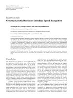
(c) Subspace order p
The order p plays a crucial role in optimising the recognition
accuracy improvement for the LS estimator.InFigure 4(a)
the word recognition accuracy is plotted against the value
of p, both for white noise at 10 (dashed line) and 20 (solid
line)dBSNR.Moreover,theoptimalvalueofp strongly de-
pends on the SNR. Hence, it is important to obtain a re-
liable estimate of the a priori SNR of the noisy signal. As
a rule of thumb, the value of p can be set approximately
equal to q/2(SNR < 10 dB), 2/3q (10 < SNR < 20 dB),
and 0.8q (SNR > 20dB). When using a variable order p, the
speech recognition accuracy considerably drops. The most
obvious explanation for this observation may be the non-
stationarities that are introduced at the level of the signal dis-
tortion and the residual noise. It is well known that speech
recognisers are very sensitive to variations of the background
noise level, more than to the absolute level of the noise
[38].
For all estimators that combine the removal of the noise
subspace with the suppression of the noise in the signal sub-

space, a different dependency is observed. In order to obtain
the best recognition rate, the value of p should be set almost
Kris Hermus et al. 13
2 4 6 8 1012 14161820
10
0
10
20
30
40
50
60
70
80
90
p
Word recognition accuracy (%)
q = 8
q
= 12
q
= 16
q
= 20
q
= 8
q
= 12
q
= 16

q
= 20
(a) LS
2 4 6 8 1012 14161820
10
0
10
20
30
40
50
60
70
80
90
p
Word recognition accuracy (%)
q = 8
q
= 12 q = 16
q = 20
q
= 8
q
= 12
q
= 16
q
= 20
(b) MV

Figure 4: Word recognition accuracy for the SVD-based enhanced signal as a function of the order p of the enhanced Hankel matrix, for
different values of q. A solid line is used for noisy speech at 20 dB SNR and a dashed line for 10 dB SNR. (a) LS estimator. (b) MV estimator
(representative of all estimators that perform noise reduction in the signal subspace).
equal to q (no nulling of the noise subspace in this case). In
general, it is observed that with increasing p/q, the recog-
nition rate gradually saturates to reach its maximal value at
p
≈ q.ThisisillustratedinFigure 4(b) for the MV esti-
mator. A similar behaviour is observed for the other estima-
tors that perform noise reduction in the signal subspace. The
most plausible explanation for this observation is that trun-
cation introduces signal distortions (e.g., gaps in the spec-
trum of the enhanced signal) that compromise a proper de-
coding with the clean-speech acoustic models. Note that this
observation is independent of the SNR of the input signal.
Using a variable order p instead of a fixed one has almost no
influence on the recognition rates.
6. CONCLUSION
Signal subspace speech enhancement has proven to be a pow-
erful and very flexible tool, both for increasing the speech in-
telligibility in speech communications applications and for
improving the accuracy of automatic speech recognisers in
additive noise environments. In this paper we reviewed the
basic theory of subspace filtering and compared the perfor-
mance of the most common optimisation criteria. We de-
rived a theoretical estimator to experimentally assess an up-
per bound to the performance that can be achieved by any
subspace-based method, both for the white and the coloured
noise case. We called this the optimal estimator.
The simulations as well as the automatic speech recog-

nition (ASR) experiments that were described in this paper
have given a better insight in the potential of subspace-based
speech enhancement techniques in general, and in the rela-
tive performance of the available estimators in particular.
It was found that KLT-based speech enhancement is
to be preferred over FFT-based (i.e., spectral subtraction)
algorithms, even though the latter operates at a (much) lower
computational lo ad. As described in earlier studies [6], sub-
space filtering produces much less musical noise than spec-
tral subtraction does. Also, for improved speech recognition
accuracy in noisy environments, SVD-based speech enhance-
ment turned out to be highly competitive with spectral sub-
traction.
Overall, the MV estimator—including its generalisation
to the TDC estimator—and the SDC estimator proved to
give the best results. However, the difference in performance
with the optimal estimator remains significantly high in the
framework of robust speech recognition, which motivates
further research in this respect. The experiments further
showed that a truncation of the signal observation matrix
(i.e., nulling of the noise subspace) is only advisable for pure
speech enhancement applications but not for speech recog-
nition.
We believe that the use of more advanced noise estima-
tion techniques and further integration of the subspace filter-
ing into the ASR preprocessing module will lead to improved
performance.
ACKNOWLEDGMENT
The authors would like to thank Peter Karsmakers for his
help in carrying out the computer simulations.

REFERENCES
[1] D. W. Tufts, R. Kumaresan, and I. Kirsteins, “Data adaptive
signal estimation by singular value decomposition of a data
matrix,” Proceedings of the IEEE, vol. 70, no. 6, pp. 684–685,
1982.
[2] J. A. Cadzow, “Signal enhancement—a composite property
mapping algorithm,” IEEE Transactions on Acoustics, Speech,
and Signal Processing, vol. 36, no. 1, pp. 49–62, 1988.
14 EURASIP Journal on Advances in Signal Processing
[3] M. Dendrinos, S. Bakamidis, and G. Carayannis, “Speech en-
hancement from noise: a regenerative approach,” Speech Com-
munication, vol. 10, no. 1, pp. 45–57, 1991.
[4] B. De Moor, “The singular value decomposition and long and
short spaces of noisy matrices,” IEEE Transactions on Signal
Processing, vol. 41, no. 9, pp. 2826–2838, 1993.
[5] S. Van Huffel, “Enhanced resolution based on minimum vari-
ance estimation and exponential data modeling,” Signal Pro-
cessing, vol. 33, no. 3, pp. 333–355, 1993.
[6] Y. Ephraim and H. L. Van Trees, “A sig n al subspace approach
for speech enhancement,” IEEE Transactions on Speech and Au-
dio Processing, vol. 3, no. 4, pp. 251–266, 1995.
[7] Y. Hu and P. Loizou, “Perceptual weighting motivated sub-
space based speech enhancement approach,” in Proceedings of
International Conference on Spoken Language Processing (IC-
SLP ’02), pp. 1797–1800, Denver, Colo, USA, September 2002.
[8] F. Jabloun and B. Champagne, “Incorporating the human
hearing properties in the signal subspace approach for speech
enhancement,” IEEE Transactions on Speech and Audio Process-
ing, vol. 11, no. 6, pp. 700–708, 2003.
[9] Y. Hu and P. C. Loizou, “A perceptually motivated approach

for speech enhancement,” IEEE Transactions on Speech and Au-
dio Processing, vol. 11, no. 5, pp. 457–465, 2003.
[10] S. H. Jensen, P. C. Hansen, S. D. Hansen, and J. A. Sørensen,
“Reduction of broad-band noise in speech by truncated
QSVD,” IEEE Transactions on Speech and Audio Processing,
vol. 3, no. 6, pp. 439–448, 1995.
[11] A. Rezayee and S. Gazor, “An adaptive KLT approach for
speech enhancement,” IEEE Transactions on Speech and Audio
Processing, vol. 9, no. 2, pp. 87–95, 2001.
[12] H. Lev-Ari and Y. Ephraim, “Extension of the signal subspace
speech enhancement approach to colored noise,” IEEE Signal
Processing Letters, vol. 10, no. 4, pp. 104–106, 2003.
[13] P. S. K. Hansen, P. C. Hansen, S. D. Hansen, and J. A. Sørensen,
“Experimental comparison of signal subspace based noise re-
duction methods,” in Proceedings of IEEE Internat ional Confer-
ence on Acoustics, Speech, and Sig nal Processing (ICASSP ’99),
vol. 1, pp. 101–104, Phoenix, Ariz, USA, March 1999.
[14] J. Huang and Y. Zhao, “Energy-constrained signal subspace
method for speech enhancement and recognition,” IEEE Sig-
nal Processing Letters, vol. 4, no. 10, pp. 283–285, 1997.
[15] K. Hermus, W. Verhelst, and P. Wambacq, “Optimized sub-
space weighting for robust speech recognition in additive
noise environments,” in Proceedings of 6th Internat ional Con-
ference on Spoken Language Processing (ICSLP ’00), vol. 3, pp.
542–545, Beijing, China, October 2000.
[16] K. Hermus and P. Wambacq, “Assessment of signal subspace
based speech enhancement for noise robust speech recogni-
tion,” in Proceedings of IEEE International Conference on Acous-
tics, Speech, and Signal Processing (ICASSP ’04) , vol. 1, pp. 945–
948, Montreal, Quebec, Canada, May 2004.

[17] I. Dologlou and G. Carayannis, “Physical interpretation of sig-
nal reconstruction from reduced rank matrices,” IEEE Trans-
actions on Signal Processing, vol. 39, no. 7, pp. 1681–1682,
1991.
[18] P. C. Hansen and S. H. Jensen, “FIR filter representations of
reduced-rank noise reduction,” IEEE Transactions on Signal
Processing, vol. 46, no. 6, pp. 1737–1741, 1998.
[19] Y. Ephraim and H. L. Van Trees, “A signal subspace approach
for speech enhancement,” in Proceedings of IEEE International
Conference on Acoustics, Speech, and Signal Processing (ICASSP
’93), vol. 2, pp. 355–358, Minneapolis, Minn, USA, April 1993.
[20] K. Hermus, “Signal subspace decompositions for perceptual
speech and audio processing,” Ph.D. dissertation, Katholieke
Universiteit Leuven, ESAT, Leuven-Heverlee, Belgium, De-
cember 2004.
[21] S. Doclo and M. Moonen, “GSVD-based optimal filtering
for single and multimicrophone speech enhancement,” IEEE
Transactions on Signal Processing, vol. 50, no. 9, pp. 2230–2244,
2002.
[22] I. Y. Soon, S. N. Koh, and C. K. Yeo, “Noisy speech enhance-
ment using discrete cosine transform,” Speech Communica-
tion, vol. 24, no. 3, pp. 249–257, 1998.
[23] J. Rissanen, “Modeling by shortest data description,” Automat-
ica, vol. 14, no. 5, pp. 465–471, 1978.
[24] S. Bakamidis, M. Dendrinos, and G. Carayannis, “SVD anal-
ysis by synthesis of harmonic signals,” IEEE Transactions on
Signal Processing, vol. 39, no. 2, pp. 472–477, 1991.
[25] R. Martin, “Noise power spectral density estimation based on
optimal smoothing and minimum statistics,” IEEE Transac-
tions on Speech and Audio Processing, vol. 9, no. 5, pp. 504–512,

2001.
[26] I. Cohen, “Noise spectrum estimation in adverse environ-
ments: improved minima controlled recursive averaging,”
IEEE Transactions on Speech and Audio Processing, vol. 11,
no. 5, pp. 466–475, 2003.
[27] S. Rangachari, P. C. Loizou, and Y. Hu, “A noise estimation al-
gorithm with rapid adaptation for highly non-stationary envi-
ronments,” in Proceedings of IEEE International Conference on
Acoustics, Speech, and Signal Processing (ICASSP ’04), vol. 1,
pp. 305–308, Montreal, Quebec, Canada, May 2004.
[28] G. Golub and C. Van Loan, Eds., Matrix Computations, Johns
Hopkins University Press, Baltimore, Md, USA, 1983.
[29] P. C. Hansen and S. H. Jensen, “Prewhitening for rank-
deficient noise in subspace methods for noise reduction,” IEEE
Transactions on Signal Processing, vol. 53, no. 10, pp. 3718–
3726, 2005.
[30] U. Mittal and N. Phamdo, “Signal/noise KLT based approach
for enhancing speech degraded by colored noise,” IEEE Trans-
actions on Speech and Audio Processing, vol. 8, no. 2, pp. 159–
167, 2000.
[31] Y. Hu and P. C. Loizou, “A subspace approach for enhancing
speech corrupted by colored noise,” in Proceedings of IEEE In-
ternational Conference on Acoustics, Speech, and Signal Process-
ing (ICASSP ’02), vol. 1, pp. 573–576, Orlando, Fla, USA, May
2002.
[32] Y. Hu and P. C. Loizou, “A generalized subspace approach for
enhancing speech corrupted by colored noise,” IEEE Transac-
tions on Speech and Audio Processing, vol. 11, no. 4, pp. 334–
341, 2003.
[33] G. S. Kang and L. J. Fransen, “Quality improvement of LPC-

processed noisy speech by using spectral subtraction,” IEEE
Transactions on Acoustics, Speech, and Signal Processing, vol. 37,
no. 6, pp. 939–942, 1989.
[34] Linguistic Data Consortium (LDC), nn.
edu.
[35] H G. Hirsch and D. Pearce, “The AURORA experimental
framework for the performance evaluation of speech recogni-
tion systems under noisy conditions,” in Proceedings of Inter-
national Speech Communication Association (ISCA) Workshop:
Authomatic Speech Recognition: Challanges for the New Mille-
nium (ASR ’00), pp. 181–188, Paris, France, September 2000.
[36] K. Demuynck, “Extracting, modelling and combining infor-
mation in speech recognition,” Ph.D. dissertation, Katholieke
Universiteit Leuven, ESAT, Leuven-Heverlee, Belgium, Febru-
ary 2001.
Kris Hermus et al. 15
[37] J. Duchateau, K . Demuynck, and D. Van Compernolle,
“Fast and accurate acoustic modelling with semi-continuous
HMMs,” Speech Communication, vol. 24, no. 1, pp. 5–17, 1998.
[38] Y. Gong, “Speech recognition in noisy environments: a sur-
vey,” Speech Communication, vol. 16, no. 3, pp. 261–291, 1995.
Kris Hermus wasborninAsse,Belgium,
in 1974. He received the M.S. and Ph.D.
degrees in electrical engineering from the
Katholieke Universiteit Leuven (Belgium)
in 1997 and 2004, respectively. Currently,
he is a postdoctoral research fellow of the
Institute for the Promotion of Innovation
by Science and Technology, Flanders (IWT-
Flanders) affiliated with the Speech Process-

ing Research Group of the Electrical Engi-
neering Depart ment (ESAT), Katholieke Universiteit Leuven. His
research interests are in the area of digital signal processing tech-
niques for automatic speech recognition and for speech/audio
modelling and coding.
Patrick Wambacq received the M.S. and
Ph.D. degrees in electrical engineering from
the Katholieke Universiteit Leuven (Bel-
gium) in 1980 and 1985, respectively. From
1980 to 1998 his main interests were im-
age processing in general, and automatic
visual inspection more specifically. Since
1998, he heads the Speech Processing Re-
search Group of the Electrical Engineer-
ing Department (ESAT), Katholieke Univer-
siteit Leuven, with research in the areas of robust speech recogni-
tion, spontaneous speech recognition, new architectures for recog-
nition, speaker adaptation, clinical and educational applications of
speech recognition, and speech and audio modelling.
Hugo Van hamme received the Electrical
Engineering degree from the Vrije Univer-
siteit Brussel, Belgium, in 1987, the Mas-
ter’s of Science degree in electrical engineer-
ing from Imperial College, London, in 1988,
and the Ph.D degree from the Vrije Uni-
versiteit Brussel in 1992. He joined Lernout
& Hauspie Speech Products in 1993, where
he held the positions of Researcher, Project
Leader, Director, and Senior Director of Re-
search. In 2001, he joined ScanSoft as Head of the Automotive

Group. Since 2002, he has been full-time Professor at the Katholieke
Universiteit Leuven. His research interests are in the areas of robust
automatic speech recognition and speech processing techniques for
learning applications.