Báo cáo hóa học: " Research Article Incremental Support Vector Machine Framework for Visual Sensor Networks" pptx

Hindawi Publishing Corporation
EURASIP Journal on Advances in Signal Processing
Volume 2007, Article ID 64270, 15 pages
doi:10.1155/2007/64270
Research Article
Incremental Support Vector Machine Framework for
Visual Sensor Networks
Mariette Awad,
1, 2
Xianhua Jiang,
2
and Yuichi Motai
2
1
IBM Systems and Technology Group, Department 7t Foundry, Essex Junction, VT 05452, USA
2
Department of Electrical and Computer Engineering, The University of Vermont, Burlington, VT 05405, USA
Received 4 January 2006; Revised 13 May 2006; Accepted 13 August 2006
Recommended by Ching-Yung Lin
Motivated by the emerging requirements of surveillance networks, we present in this paper an incremental multiclassification
support vector machine (SVM) technique as a new framework for action classification based on real-time multivideo collected by
homogeneous sites. The technique is based on an adaptation of least square SVM (LS-SVM) formulation but extends beyond the
static image-based learning of current SVM methodologies. In applying the technique, an initial supervised offline learning phase
is followed by a visual behavior data acquisition and an online learning phase during which the cluster head performs an ensemble
of model aggregations based on the sensor nodes inputs. The cluster head then selectively switches on designated sensor nodes
for future incremental learning. Combining sensor data offers an improvement over single camera sensing especially when the
latter has an occluded view of the target object. The optimization involved alleviates the burdens of power consumption and com-
munication bandwidth requirements. The resulting misclassification error rate, the iterative error reduction rate of the proposed
incremental learning, and the decision fusion technique prove its validity when applied to visual sensor networks. Furthermore,
the enabled online learning allows an adaptive domain knowledge insertion and offers the advantage of reducing both the model
training time and the information storage requirements of the overall system which makes it even more attractive for distributed

sensor networks communication.
Copyright © 2007 Mariette Awad et al. This is an open access article distributed under the Creative Commons Attribution License,
which permits unrestricted use, distribution, and reproduction in any medium, provided the original work is properly cited.
1. INTRODUCTION
Visual sensor networks with embedded computing and com-
munications capabilities are increasingly the focus of an
emerging research area aimed at developing new network
structures and interfaces that drive novel, ubiquitous, and
distributed applications [1]. These applications often at-
tempt to bridge the last interconnection between the outside
physical world and the World Wide Web by deploying sen-
sor networks in dense or redundant formations that alleviate
hardware failure and loss of information.
Machine learning in visual sensor networks is a very use-
ful technique if it reduces the reliance on a priori knowledge.
However, it is also very challenging to implement. Addition-
ally it is subject to the constraints of computing capabili-
ties, fault tolerance, scalability, topology, security and power
consumption [2, 3]. Even effective algorithms for automated
knowledge acquisition like the ones presented by Duda et al.
[4] face limitations when applied to sensor networks due to
the distributed nature of the data sources and their hetero-
geneity.
The adequacy of a machine learning model is measured
by its ability to provide a good fit for the training data as
well as correct prediction for data that was not included in
the training samples. Constructing an adequate model starts
with the thorough offline collection of a dataset that rep-
resents the learning-from-examples paradigm. The training
process can therefore become very time consuming and re-

source intensive. Furthermore, the model will need to be pe-
riodically revalidated to insure its accuracy in data dissemi-
nation and aggregation.
The incorporation of incremental modular algorithms
into the sensor network architecture would improve ma-
chine learning and simplify network model implementation.
The reduced training period will provide the system with
added flexibility and the need for periodic retraining will
be minimized or eliminated. Within the context of incre-
mental learning, we present a novel technique that extends
2 EURASIP Journal on Advances in Signal Processing
traditional SVM beyond its existing static image-based learn-
ing methodologies to handle multiple action classification.
We opted to investigate behavior learning because it is
useful for many current and potential applications. They
range from smart surveillance [5] to remote monitoring of
elderly patients in healthcare centers and from building a
profile of people manners [6] to elucidating rodent behav-
ior under drug effects [7],andsoforth.Forillustrationpur-
poses, we have applied our technique to learn the behavior of
an articulated humanoid through video footage captured by
monitoring camera sensors. We have then tested the model
for its accuracy in classifying incremental articulated mo-
tion. The initial supervised offline learning phase was fol-
lowed by a visual behavior data acquisition and an online
learning phase. In the latter, the cluster head performed an
ensemble of model aggregations based on the information
provided by the sensor nodes. Model updates are executed in
order to increase its classification accuracy of the model and
to selectively switch on designated sensor nodes for future

incremental lear ning.
To the best of our knowledge, no prior work has used an
adaptation of LS-SVM with a multiclassification objective for
behavior learning in an image sensor network. The contribu-
tion of this study is the derivation of this unique incremen-
tal multiclassification technique that leads to an extension of
SVM beyond its current static image-based learning method-
ologies.
This paper is organized as follows: Section 2 presents
an overview of SVM principles and related techniques.
Section 3 covers our unique multiclassification procedure
and Section 4 introduces our proposed incremental SVM.
Section 5 then describes the visual sensor network topol-
ogy and operations. Section 6 summarizes the experimental
results. Finally, Section 7 contains concluding remarks and
outlines our plans for follow-on work.
2. SVM PRINCIPLES AND RELATED STUDIES
Our study focuses on SVM as a prime classifier for an in-
cremental multiclassification mechanism for sequential in-
put video in a visual sensor network. The selection of SVM
as a multiclassification technique is due to several of its main
advantages: SVM is computationally efficient, highly resis-
tant to noisy data, and offers generalization capabilities [8].
These advantages make SVM an attractive candidate for im-
age sensor network applications where computing power is
a constraint and captured data is potentially corrupted with
noise.
Originally designed for binary classification, the SVM
techniques were invented by Boser, Guyon, and Vapnik and
were introduced during the Computational Learning Theory

(COLT) Conference of 1992 [8]. SVM has its roots in statis-
tical learning theory and constructs its solutions in terms of
a subset of the training input. Furthermore, it is similar to
neural networks from a structural perspective but differs in
its learning technique. SVM tries to minimize the confidence
interval and keep the t raining error fixed while maximizing
the distance between the calculated hyperplane and the near-
est data p oints known as support vectors. These support vec-
tors define the margins and summarize the remaining data,
which can then be ignored.
The complexity of the classification task will thus de-
pend on the number of support vectors rather than on the
dimensionality of the input space and this helps prevent
over-fitting. Traditionally, SVM was considered for unsu-
pervised offline batch computation, binary classifications,
regressions, and structural risk minimization (SRM) [8].
Adaptations of SVM were applied to density estimation
(Vapnik and Mukherjee [9]), Bayes point estimation (Her-
brich et al. [10]), and transduction [4] problems. Researchers
also extended the SVM concepts to address error margin
(Platt [11]), efficiency (Suykens and Vandewalle [12]), mul-
ticlassification [13], and incremental learning (Ralaivola and
d’Alch’e-Buc, Cauwenberghs and Poggio, resp., [14, 15]).
In its most basic definition, a classification task is one in
which the learner is trained based on labeled examples and
is expec ted to classify subsequent unlabeled data. In building
the mathematical derivation of a standard SVM classification
algorithm, we let T
={(x
1

, y
1
), ,(x
N
, y
N
)} where x
i
∈ R
n
is a training set with attributes or features  f
1
, f
2
, , f
n
.Fur-
thermore, let T
+
={x
i
| (x
i
, y
i
) ∈ T and y
i
= 1} and T =
{
x

i
| (x
i
, y
i
) ∈ T and y
i
=−1} be the set of positive and
negative training examples, respectively. A separating hyp er-
planeisgivenbyw
· x
i
+ b = 0. For a correct classification,
all x
i
’s must satisfy y
i
(w · x
i
+ b) ≥ 0. Among all such planes
satisfying this condition, SVM finds the optimal hyperplane
P
0
where the margin distance between the decision plane
and the closest sample points is maximal. P
0
is defined by
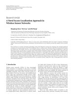
its slope w and should be situated as indicated in Figure 1(a)
equidistant from the closest point on either side. Let P
+

and
P
−
be 2 additional planes that are parallel to P
0
and include
the support vectors. P
+
and P
−
are defined, respectively, by
w
· x
i
+ b = 1, w · x
i
+ b =−1. All points x
i
should satisfy
w
· x
i
+ b ≥ 1fory
i
= 1, or w · x
i
+ b ≤ 1fory
i
=−1.
Thus combining the conditions for all points x

i
we have y
i
(w · x
i
+ b) ≥ 1. The distances from the origin to the three
planes P
0
, P
+
,andP
−
are, respectively, |b − 1|/w, |b|/w,
and
|b +1|/w.
Equations (1) through (6) presented below are based on
Forsyth and Ponce [16]. The optimal plane is found by min-
imizing (1) subject to the constraint in (2)
objective function
1
2
w
2
,(1)
constraint: y
i

wx
i
+ b


≥
1. (2)
Any new data point is then classified by the decision func-
tion in (3),
decision function: f (x)
= sign(w · x + b). (3)
Since the objective function is quadratic, this constrained
optimization is solved by Lagrange multipliers method. The
goal is to minimize with respect to w, b, and the Lagrange
Mariette Awad et al. 3
Separating
hyperplane
P
+
P
0
P
Support vectors
2
w
(a)
Separating
hyperplane
P
1
P
0
P
2

2
[wb]
(b)
Figure 1: Standard versus proposed binary classification using regularized LS-SVM.
coefficients α
i
:
L
p
(w, b, α) =
1
2
w
2
−
N

i=1
α
i

y
i

wx
i
+ b

− 1


. (4)
Let (∂/∂w)L
P
(w, b) = 0, ( ∂/∂b)L
p
(w, b) = 0.
Thus
w
=
N

j=1
α
j
y
j
x
j
. (5)
Substituting (5) into (3) allows us to rewrite the decision
function as
f (x)
= sign(w · x + b) = sign

N

i=1
α
i
· y

i
· x · x
i
+ b

.
(6)
3. PROPOSED MULTICLASSIFICATION SVM
We extend the standard SVM to use it for multiclassification
tasks.
The objective function now becomes
1
2
c

m=1

w
T
m
· w
m
+ b
m
· b
m

+ λ
N


i=1
c

m=y
i

e
m
i

2
. (7)
We added to the objective function in (1) the plane in-
tercept term b as well as an error term e and its penalty pa-
rameter λ. Adding b into the objective function as shown in
(7) will uniquely define the plane P
0
by its slope w and inter-
cept b. As shown in Figure 1(b), the planes P
+
and P
−
are
not the decision boundaries anymore as is the case in the
standard binary classification case of Figure 1(a). Instead in
this scenario, the new planes P
1
and P
2
are located at a max-

imal margin distance of 2/[
wb
]fromP
0
. The error term
e accounts for the possible soft misclassification occurring
with data points violating the constraint of (2). Adding the
penalty par ameter λ as a cost to the error term e greatly im-
pacts the classifier performance. It enables the regulation of
the error term, e, for behavior classification dur ing the train-
ing phase. The selection of λ can be found heuristically or
by a grid search. Large λ values favor less smooth solutions
that drive large w values. Hsu and Lin [17] showed that SVM
accuracy rates were influenced by the selection of λ which
varies in ranges depending on the problem under investiga-
tion.
Similarly to traditional LS-SVM, we carry the optimiza-
tion step with an equality constraint, but we drop the La-
grange multipliers.
Selecting the multiclassification objective function, the
constraint function becomes

w
T
y
i
· x
i

+ b

y
i
=

w
T
m
· x
i

+ b
m
+2− e
m
i
. (8)
Similar to a regularized LS-SVM, the problem solution now
becomes equal to the rate of change in the value of the objec-
tive function. In this approach, we do not solve the equation
for the support vectors that correspond to the nonzero La-
grange multipliers in traditional SVM. Instead our solution
now seeks to define two planes P
1
and P
2
around which clus-
ter the data points. The classification of data points will be
performed by assigning them to the closest parallel planes.
Since it is a multiclassification problem, a data point is as-
signed to a specific class after being tested against all existing

classes using the decision function of (9). This specific class
4 EURASIP Journal on Advances in Signal Processing
has the largest value of (9),
f (x)
= arg max
m

w
T
m
· x

+ b
m

, m = 1, , c. (9)
Figure 1 compares a standard SVM binar y classification
to the proposed technique.
Substituting (8) into (7), we get
L(w, b)
=
1
2
c

m=1

w
m
· w

m
+ b
m
· b
m

+ λ
N

i=1
c

m=y
i

w
y
i
− w
m

x
i
+

b
y
i
− b
m


−
2

2
.
(10)
Taking partial derivatives of L(w, b)withrespecttobothw
and b,
∂L(w, b)
∂w
n
= 0,
∂L(w, b)
∂b
n
= 0. (11)
Choosing λ
= 1/2 and defining
a
i
=
⎧
⎨
⎩
1, y
i
= n,
0, y
i

= n,
(12)
equation (11)becomes
w
n
+
N

i=1


−
x
i
· x
T
i

w
y
i
− w
n

− x
i

b
y
i

− b
n

− 2x
i

1 − a
i

+
c

m=y
i

x
i
x
T
i

w
y
i
−w
m

+x
i


b
y
i
−b
m

+2x
i

a
i

=
0,
b
n
+
N

i=1

−

x
T
i

w
y
i

− w
n

+

b
y
i
− b
n

+2

1 − a
i

+
c

m=y
i

x
T
i

w
y
i
− w

m

+

b
y
i
− b
m

+2

a
i

=
0.
(13)
Let us define
S
w
:=
N

i=1

−

w
y

i
− w
n

x
2
i

1 − a
i

+
c

m=y
i

w
y
i
− w
m

x
2
i
a
i

=⇒

S
w
=−
N

i=1

w
y
i
− w
n

x
2
i
+
q(n)

p=1
x
2
i
p
c

n=1

w
n

− w
m

.
(14)
A similar argument shows that
S
b
:=
N

i=1

−

b
y
i
− b
n

x
i

1 − a
i

+
c


m=y
i

b
y
i
− b
m

x
i
a
i

=⇒
S
b
=−
N

i=1

b
y
i
− b
n

x
i

+
q(n)

p=1
x
i
p
c

m=1

b
n
− b
m

.
(15)
Finally,
S
2
:=
N

i=1

2x
i

1 − a

i

−
c

m=y
i
2x
i
a
i

=⇒
S
2
=
N

i=1
2x
i
−
q(n)

p=1
2x
i
p
−
q(n)


p=1
c

m=1
2x
i
p
= 2
N

i=1
x
i
− c
q(n)

p=1
x
i
p
.
(16)
Applying similar reasoning for b, we can rearrange (13)to
get

I +
N

i=1

x
i
x
T
i
+ c
q(n)

p=1
x
i
p
x
T
i
p

w
n
+ b
n

N

i=1
x
i
+ c
q(n)


p=1
x
i
p

=
N

i=1
x
i
x
T
i
w
y
i
+
q(n)

p=1
x
i
p
x
T
i
p
c


m=1
w
m
+
N

i=1
x
i
b
y
i
+
q(n)

p=1
x
i
p
c

m=1
b
m
+2
N

i=1
x
i

− 2c
q(n)

p=1
x
i
p
,

N

i=1
x
T
i
+ c
q(n)

p=1
x
T
i
p

w
n
+ b
n

1+N + cq(n)


=
N

i=1
x
T
i
w
y
+
q(n)

p=1
x
T
i
p
c

m=1
w
m
+
N

i=1
b
y
i

+ q(n)
c

m=1
b
m
+2(N − c)q(n).
(17)
To rew r i t e ( 17) in a matrix format, we use the series of
definitions as mentioned below.
Let f denote the dimensions of feature space and q(n)
the size of class n,and
(1) let C be a diagonal matrix of size ( f
∗
c)by(f
∗
c),
C
=
⎡
⎢
⎢
⎢
⎢
⎢
⎢
⎢
⎣
c
1

0 · 00
0 c
2
· 00
·····
00·· 0
00
· 0 c
c
⎤
⎥
⎥
⎥
⎥
⎥
⎥
⎥
⎦
, (18)
C is composed of matrix c
n
such that c
n
is a square
matrix of size f ,
c
n
= I +
N


i=1
x
i
x
T
i
+ c
q(n)

p=1
x
i
p
x
T
i
p
; (19)
(2) let D be a diagonal matrix of size ( f
∗
c)byc,
D
=
⎡
⎢
⎢
⎢
⎢
⎢
⎢

⎢
⎣
d
1
0 · 00
0 d
2
· 00
·····
00·· 0
00
· 0 d
c
⎤
⎥
⎥
⎥
⎥
⎥
⎥
⎥
⎦
, (20)
Mariette Awad et al. 5
D is composed of the column vector d
n
of length f
such that
d
n

=
N

i=1
x
i
+ c
d(n)

p=1
x
i
p
; (21)
(3) let G be a square matrix of size ( f
∗
c)by(f
∗
c).
G is composed of matrix g
n
of size f by c such that
G
=
⎡
⎢
⎢
⎢
⎢
⎢

⎢
⎢
⎣
g
1
·
·
·
g
c
⎤
⎥
⎥
⎥
⎥
⎥
⎥
⎥
⎦
,
g
n
=
⎡
⎣

q(1)

p=1
x

i
p
x
T
i
p
+
q(n)

p=1
x
i
p
x
T
i
p

···

q(c)

p=1
x
i
p
x
T
i
p

+
q(n)

p=1
x
i
p
x
T
i
p

⎤
⎦
;
(22)
(4) let H be a square matrix of size ( f
∗
c)byc.
H is composed of the row vector h
n
of length c,
H
=
⎡
⎢
⎢
⎢
⎢
⎢

⎣
h
1
·
·
·
h
c
⎤
⎥
⎥
⎥
⎥
⎥
⎦
,
h
n
=
⎡
⎣
q(1)

p=1
x
i
p
+
q(n)


p=1
x
i
p
q(2)

p=1
x
i
p
+
q(n)

p=1
x
i
p
···
q(c)

p=1
x
i
p
+
q(n)

p=1
x
i

p
⎤
⎦
;
(23)
(5) let E be a column vector made from
E
=
⎡
⎢
⎢
⎢
⎢
⎢
⎣
e
1
·
·
·
e
c
⎤
⎥
⎥
⎥
⎥
⎥
⎦
, e

n
=−2
N

i=1
x
i
+2c
q(n)

p=1
x
i
p
; (24)
(6) let Q be a square matrix of size c by c,
Q
=
⎡
⎢
⎢
⎢
⎢
⎢
⎣
q
1
·
·
·

q
c
⎤
⎥
⎥
⎥
⎥
⎥
⎦
, (25)
Q is made from the row vector q
n
of length c
q
n
=


q(1) + q(n)

···

q(c)+q(n)


(26)
(7) let U be a column vector of size c by 1,
U
=
⎡

⎢
⎢
⎢
⎢
⎢
⎣
u
1
·
·
·
u
c
⎤
⎥
⎥
⎥
⎥
⎥
⎦
, (27)
U is made from
u
n
=−2

N − cq(n)

; (28)
(8) let R be a square matrix of size c,

R
=
⎡
⎢
⎢
⎢
⎢
⎢
⎣
r
1
0000
0 r
2
000
00
· 00
000
· 0
0000r
c
⎤
⎥
⎥
⎥
⎥
⎥
⎦
, (29)
R is made from

r
n
= 1+N + cq(n). (30)
The above definitions allow us to manipulate (17)and
rewrite as
(C
− G)W +(D − H)B = E,
(D
− H)W +(R − Q)B = U.
(31)
Solving for W, B,weget

W
B

=

(C − G)(D − H)
(D
− H)
T
(R − Q)

−1

E
U

. (32)
We define matrix A to be

A
=

(C − G)(D − H)
(D
− H)
T
(R − Q)

(33)
and L to be
L
=

E
U

. (34)
This will allow us to rewrite (17)inaverycompactway:

W
B

=
A
−1
L. (35)
Equation (35) provides the separating hyperplane slopes
and intercepts values for the different c classes. The hyper-
plane is uniquely defined based on matrices A and L and does

not depend on the support vectors or the Lagrange multipli-
ers.
4. PROPOSED INCREMENTAL SVM
In traditional SVM, every new image sequence (x
N+1
) that
is captured gets incorporated into the input space and the
hyperplane parameters are recomputed accordingly. Clearly,
this approach is computationally very expensive for a visual
sensor network. To maintain an acceptable balance between
storage, accuracy, and computation time, we propose an in-
cremental methodology to appropriately dispose of the re-
cently acquired image sequences.
4.1. Incremental strategy for sequential data
During sequential data processing, and whenever the model
needs to be updated, each incremental sequence will alter
matrices C, G, D, H, E, R, Q,andU in (32)and(33). For
6 EURASIP Journal on Advances in Signal Processing
illustrative purposes, let us consider a recently acquired data
x
N+1
belonging to class t.Equation(35) then becomes

W
B

n
=

(C+ΔC)−(G+ΔG)(D+ΔD)−(H+ΔH)

(D+ΔD)
−(H +ΔH)(R+ΔR)−(Q+ΔQ)

−1
×

E + ΔE
U + ΔU

.
(36)
To assist in the mathematical manipulation, we define the
following matrices:
I
c
=
⎡
⎢
⎢
⎢
⎢
⎢
⎢
⎢
⎢
⎢
⎢
⎣
100 0 · 0
010 0

· 0
··· · ··
0001+c · 0
··· · ··
000 0 · 1
⎤
⎥
⎥
⎥
⎥
⎥
⎥
⎥
⎥
⎥
⎥
⎦
,
I
t
=
⎡
⎢
⎢
⎢
⎢
⎢
⎢
⎢
⎢

⎢
⎢
⎣
00· 1 · 0
00
· 1 · 0
······
11· 2 · 1
······
00· 1 · 0
⎤
⎥
⎥
⎥
⎥
⎥
⎥
⎥
⎥
⎥
⎥
⎦
, I
e
=
⎡
⎢
⎢
⎢
⎢

⎢
⎢
⎢
⎣
1
1
·
1 − c
·
1
⎤
⎥
⎥
⎥
⎥
⎥
⎥
⎥
⎦
.
(37)
We can then rewrite the incremental change as follows:
ΔC
=

x
N+1
x
T
N+1


I
c
, ΔG =

x
N+1
x
T
N+1

I
t
,
ΔD
= x
N+1
I
c
, ΔH = x
T
N+1
I
t
,
ΔE
=−2x
N+1
I
e

, ΔR = I
c
,
ΔQ
= I
t
, ΔU =−2I
e
.
(38)
The new model parameters now become

W
B

n
=
⎡
⎣
A +
⎡
⎣

x
N+1
x
T
N+1

I

c
− I
t

x
T
N+1

I
c
− I
t

x
T
N+1

I
c
− I
t

I
c
− I
t

⎤
⎦
⎤

⎦
−1
×
⎡
⎣
L +
⎡
⎣
−
2x
N+1
I
e
−2I
e
⎤
⎦
⎤
⎦
.
(39)
Let
ΔA
=
⎡
⎣

x
N+1
x

T
N+1

I
c
− I
t

x
T
N+1

I
c
− I
t

x
T
N+1

I
c
− I
t

I
c
− I
t


⎤
⎦
,
ΔL
=
⎡
⎣
−
2x
N+1
I
e
−2I
e
⎤
⎦
.
(40)
We thus arrive to

W
B

n
= (A + ΔA)
−1
(L + ΔA). (41)
Equation (41) shows that the separating hyperplanes
slopes and intercepts for the different c classes of (35)canbe

efficiently updated just by using the old model parameters.
The incremental change introduced by the recently acquired
data stream is incorporated as “perturbation” to the initially
developed system parameters.
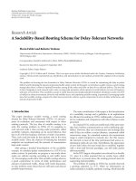
Figure 2(a) represents the plane orientation before the
acquisition of x
N+1
,whereasFigure 2(b) shows the effect of
x
N+1
on shifting the planes orientation whenever an update
is necessary.
After computing the model parameters, the input data
can be deleted because it is not needed for potential future
updates. This incremental approach reduces tremendously
system storage requirements and is attractive for sensor ap-
plications where online learning, low power consumption,
and storage requirements are challenging to satisfy simulta-
neously.
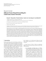
Our proposed technique, as highlighted in Figure 3,
meets the following three main requirements for incremental
learning.
(1) Our system is able to use the learned knowledge to
perform on new data sets using (35).
(2) The incorporation of “experience” (i.e., newly col-
lected data sets) in the system parameters is computationally
efficient using (41).
(3) The storage requirements for the incremental learn-
ing task are reasonable.
4.2. Incremental strategy for batch data

For incremental batch processing, the data is still acquired
incrementally, but it is stored in a buffer awaiting chunk pro-
cessing. After capturing k sequences and if the model needs
to be updated, the recently acquired data is processed and the
model is updated as described by (41). Alternately we can use
the Sherman-Morrison-Woodbury [18] generalization for-
mula described by (42) to account for the perturbation intro-
duced by matrices M and L defined such that (I +M
T
A
−1
L)
−1
exists,

A + LM
T

−1
= A
−1
− A
−1
L

I + M
T
A
−1
L


−1
M
T
A
−1
,
(42)
where
M
=

x
N+1

I
c
− I
t


I
c
− I
t


, L =

x

N+1
I

T
. (43)
Using (35)and(42), the new model can represent the in-
crementally acquired sequences according to (44),

W
B

n
=

W
B

old
+

ΔE
ΔU

+

ΔE
ΔU

−


W
B

old

×

I − A
−1
M

I + M
T
A
−1
L

−1
M
T
A
−1

.
(44)
Equation (44) shows the influence of the incremental
data on calculating the new separating hyperplane slopes and
intercept values for the different c classes.
Mariette Awad et al. 7
x

n+1
P
1
P
0
P
2
(a)
x
n+1
P
1 new
P
0 new
P
2 new
P
1
P
0
P
2
(b)
Figure 2: Effect of x
N+1
on plane orientation in case a system parameter update is needed.
Yes No
x
n+1
:

update
needed
Efficiently
computed
Stored
from prior
knowledge
Update
ΔA
=

(x
N+1
x
T
N+1
)(I
c
-I
t
) x
T
N+1
(I
c
-I
t
)
x
T

N+1
(I
c
-I
t
)(I
c
-I
t
)

ΔL =

-2x
N+1
I
e
-2I
e

Multiclass SVM

W
B

=
A
-1
L
Incremental SVM


W
B

n
= (A + ΔA)
-1
(L + ΔL)
Figure 3: Process flow for the incremental model parameter up-
dates.
5. VISUAL SENSOR NETWORK TOPOLOGY
Sensor networks, including ones for visual applications, are
generally composed of 4 layers: sensors, middleware, appli-
cation, and client levels [1, 2].Inourstudy,weproposeahi-
erarchical network topology composed of sensor nodes and
cluster head nodes. The cluster-based topology is similar to
the LEACH protocol proposed by Heinzelman et al. [19 ]in
which nodes are assumed to have limited and nonrenewable
energy resources. The sensor and application layers are as-
sumed generic. Furthermore, the sensor layer allows dynamic
configuration such as sensor rate, communication schedul-
ing, and power battery monitoring. The main func tions of
x
N+1
x
N+1
.
.
.
Sensor nodes

Classify
Classify
.
.
.
Cluster head
Decision
fusion
Figure 4: Decision fusion at cluster head level.
the application layer are to manage the sensors and the mid-
dleware and to analyze and aggregate the data as needed. The
sensor node and cluster head operations are detailed in Sec-
tions 5.1 and 5.2,respectively.
Antony [20] breaks the problem of output fusion and
multiclassifier combination into two sections: the first related
to the classifiers specifics such as number of classifiers to be
included and feature space requirements and the second per-
tains to the classifiers mechanics such as fusion techniques.
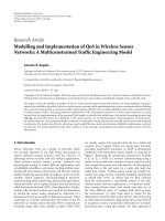
Our study focuses primarily on the latter part of the
problem and we specifically address fusion at the decision
and not at the data level. Figure 4 depicts the decision fusion
at the cluster head level. Decision fusion mainly achieves an
acceptable tradeoff between the probabilities for the “wrong
decisions” likely to occur in decision fusion systems and the
low communication bandwidth requirements needed in sen-
sor networks.
5.1. Sensor nodes operations
A sensor node is composed of an image sensor and a proces-
sor. The former can be an off-the-shelf IEEE-1394 firewire
network camera, such as the Dragonfly manufactured by

8 EURASIP Journal on Advances in Signal Processing
Local prediction to
cluster head
Image processing :
filter noise, feature
extraction
Sensor node
Cluster head
interface
Sensor
Captured image
Figure 5:Genericsensornodetopology.
Point Grey Research [21]. The latter can range from a sim-
ple embedded processor to a server for extensive computing
requirements. The sensor node can connect to the other lay-
ers using a local area network (LAN) enablement.
When the sensor network is put online, camera sensors
are expected to start transmitting captured video sequences.
It is assumed that neither gossip nor flooding is allowed at
the sensor nodes level because these communication schemes
would waste sensor energy. Camera sensors incrementally
capture two-dimensional data, preprocess it, and transmit
it directly to their cluster head node via the cluster head
interface as shown by the generic sensor node topology in
Figure 5.
Throughout the process, sensor nodes are responsible to
extract behavior features from the video image sequences.
They store the initial model parameters A, L,andW of (33),
(34), and (35), respectively, and have limited buffer capabili-
ties to store incoming data sequences.

Several studies related to human motion classification
and visual sensor networks have been published. The study
of novel extraction methods and motion tracking is poten-
tially a standalone topic [22–27]. Different sensor netw o rk
architectures were proposed to enable dynamic system archi-
tecture (Matsuyama et al. [25]), real time v isual surveillance
system (Haritaoglu et al. [26]), wide human tracking area
(Nakazawa et al. [27]), and integrated system of active cam-
era network for human tracking and face recognition (Sogo
et al. [28]).
The scope of this paper is not to propose novel feature ex-
traction techniques and motion detection. Our main objec-
tive is to demonstrate machine learning in visual sensor net-
works using our incremental SVM methodology. During the
incremental learning phase, sensor nodes need to perform
local model verification. For instance, if x
N+1
is the recently
acquired frame sequence that needs to be classified, our pro-
posed strategy would entail the following steps highlighted
in Algorithm 1.
5.2. Cluster head no de operations
The cluster head is expected to t rigger the model updates
based on an efficient meta-analysis and aggregate protocol.
A properly selected aggregation procedure can be superior to
a single classifier whose output is based on a decision fusion
of all the different classification results of the network sensor
nodes [29].
The generic cluster head architecture is outlined in Figure
6.

Performance generalization and efficiency are two im-
portant and interrelated issues in pattern recognition. We
keep track of the former by calculating its misclassification
error rate Mis
Err t i and the error reduction rate ERR t i,
where t represents the iteration index counter and i the cam-
era sensor id. The misclassification error rate refers to the
accuracy obtained with each classifier whereas the error re-
duction rate ERR
t i represents the percentage of error re-
duction obtained by combining classifiers with reference to
the best single classifier. ERR
t i reveals the per formance
trend and merit of the combined classifiers with respect to
the best single classifier. It is not necessary to have identical
Mis
Err t i for all the cameras, however it is reasonable to ex-
pect Mis
Err t i rates to decrease with incremental learning.
For the cluster head specific operations, we study 2
modes: (1) decision fusion to appropriately handle nonla-
beled data, and (2) selective sensor node switching during in-
cremental learning to reduce communication cost in the sen-
sor network. Details of the applied techniques are outlined in
Algorithm 2.
6. EXPERIMENTAL RESULTS
We validated our proposed technique in a two-stage scenario.
First, we substantiated our proposed incremental multiclas-
sification method using one camera alone to highlight its ef-
ficiency and validity relative to the retrain model. Second, we

verified our distributed information processing and decision
fusion approaches in a sensor network environment.
The data was collected according to the block diagram
of the experimental setup as shown in Figure 7. The setup
consists of a humanoid animation model that is consistent
with the standards of the International Organization for
Standardization (ISO) and the International Electrotechnical
Commission (IEC) (FCD 19774) [30]. Using a uniquely de-
veloped graphical user interface (GUI), the humanoid mo-
tion is registered in the computer based on human interac-
tion. We use kinematics models to enable correct behavior
registration with respect to adjacency constraints and relative
joint relationships. The registered behavior is used to train
themodelinanoffline mode.
To identify motion and condense the space-time frames
into uniquely defined vectors, we extract the input data by
tracking color-coded marker points tagged to 11 joints of the
humanoid as proposed in our earlier work in [30]. This ex-
traction method results in lower storage needs without af-
fecting the accuracy of behavior description since motion
detection is derived from the positional variations of the
markersrelativetopriorframes.Thisideaissomewhatsim-
ilar to silhouette analysis for shape detection as proposed by
Belongie et al. [31].
The collected raw data is an image sequence of the hu-
manoid. Each image is treated as one unit of sensory data.
For each behavior, we acquired 40 space time sequences each
comprised of 50 frames that adequately characterize the dif-
ferent behavioral classes shown in Ta ble 1.
Mariette Awad et al. 9

Step (1) During the initial training phase, the initial model parameters W
0,i
and b
0,i
based on matrices A
0,i
and L
0,i
of (32)
and (33)arestoredfortheith camera sensor in the cache memory,
A
0,i
=

(C − G)(D − H)
(D
− H)
T
(R − Q)

, L
0,i
=

E
U

.
Step (2) Each camer a attempts to correctly predict the class label of x
N+1

by using the decision function represented by (9),
f (x)
= arg max
m

w
m
· x

+ b
m

.
Step (3) Local decisions about the predicted classes are communicated to the cluster head.
Step (4) Based on the cluster head decision described in Algorithm 2, if a model update is detected, the incremental
approach described in Sections 4.1 and 4.2 is applied in order to reduce memory storage and to target faster performance,

W
B

n
= (A + ΔA)
−1
(L + ΔL)
or

W
B

n

=

W
B

old
+

ΔE
ΔU

+
⎡
⎢
⎣

ΔE
ΔU

−

W
B

old
⎤
⎥
⎦

I − A

−1
M

I + M
T
A
−1
L

−1
M
T
A
−1

.
The recently acquired image data x
N+1
is deleted after the model is updated.
Step (5) If no model updates are detected, the incrementally acquired images are stored so that they are included in future updates.
Storing these sequences will help ensure the system will always learn even after several nonincremental steps.
Algorithm 1: Sensor nodes operations.
Fusion decision to
sensor nodes
Cluster head
Decision
fusion
processor
Sensor interface
Sensor interface

Sensor interface
Sensor interface
From sensor nodes
Figure 6: Generic cluster head topology.
Table 1 lists the behavioral classes for the humanoid ar-
ticulated motions that we selected for illustration purposes
of our incremental multiclassification technique.
The limited number of training datasets is one of the
inherent difficulties in the learning methodology [32]and
therefore, we extended the sequences collected during our
experimental setup by deriving related artificial data. This
approach also allows us to test the robustness of SVM solu-
tions when applied to noisy data. The results are summarized
in the following subsections.
6.1. Analyzing sequential articulated humanoid
behaviors based on one visual sensor
We first ran two experiments based on one camer a input
in order to fi rst validate our proposed incremental multi-
classification technique. Our analysis was based on a matrix
of two models with five different experiments each. In all
instances, we did not reuse the data sequences used for train-
ing to prevent the model from becoming overtrained. The se-
quences used for testing were composed of an equal number
of frame sequences for each humanoid selected behavior as
represented in Table 1. Figure 8 represents the mar kers’ posi-
tion for the selected articulated motions of Table 1. The two
different models were defined as follows.
(i) Model 1
Incremental model: acquire and sequentially process incre-
mental frames one at a time according to the incremental

strategy highlighted in Section 4. When necessary, update the
model incrementally as proposed in Section 5. Compute the
overall misclassification error rate for all the behaviors of
Table 1 based on a subsequent test-set sequence Ts.
(ii) Model 2
Retrain model: acquire and incorporate incremental frames
in the training set. Recompute the model parameters. Com-
pute the overall misclassification error rate for all the behav-
iors based on the same subsequent test-set sequence used in
model 1.
Figure 9 shows the performance of the incremental
model as being comparable to model 2 that continuously re-
trains.
The error difference between our proposed incremental
multiclassification SVM and the retraining model is 0.5%.
Furthermore, the improved performance of model 2 is at the
expense of increased storage and computing requirements.
10 EURASIP Journal on Advances in Signal Processing
Cluster head receives the predicted class label of x
N+1
class from each camera.
(I) Dec ision fusion for nonlabeled data
Cluster head performs decision fusion based on collected data from sensor nodes. Cluster head aggregation procedure can be either
(i) majority voting: F(d
i
), or
(ii) weighted-decision fusion: F(d
i
, ψ
i

),
where F represents the aggregation module
(a) d
i
the local decision of each camera id,
(b) ψ
i
the confidence level associated with each camera. ψ
i
is evaluated using each classifier confusion matrix,
ψ
i
can be rewritten as ψ
i
=

c
j
=1
C
i
jj

c
k
=1

c
j
=1

j
=i
C
i
kj
,
where C
i
jj
is the jth diagonal element in the confusion matrix of the ith sensor node, C
i
kj
represents the number of data b elonging to
class k whereas classifier i recognized them as being class j.
Based on the cluster head final decision, instructions to update model parameters A, L,andW are then sent to the sensor nodes.
(II) Incremental learning
Step (1) Selective switching in incremental learning: if the misclassification error rate Mis
Err t i ≥ Mis Err,
cluster head can selectively switch on sensor nodes for the next sequence of data acquisition. Selective switching can be either
(1) baseline: all nodes are switched on, or
(2) strong and weak combinations: a classifier is considered weak as long as it performs better than random guessing. The
required generalization error of a classifier is (0.5
− ∂)where∂ ≥ 2 and it describes the weakness of the classifier.
ERR
t i is calculated as
ERR
=
ERR
(Best classifier)
− ERR

(Combined classifier)
ERR
(Best classifier)
∗ 100,
where ERR
(Best classifier)
is the error reduction rate observed for the best performing classifier and ERR
(Combined classifier)
is the error
reduction rate observed when all the classifiers are combined.
Step (2) If no model updates are detected, cluster head informs the sensor nodes to store the incrementally acquired images
so that they are included in future updates. Storing these s equences will help ensure the system will always learn even after
several nonincremental steps.
Step (3) Every time parameter models are not updated for consecutive instances as in step (2), an “intelligent timer” is activated to
keep track of the trend in Mis
Err t i.IfMis Err t i is not statistically increasing, the “intelligent timer” will inform the sensor nodes
to delete the incrementally acquired video sequence stored in buffer. This will reduce storage requirements and preserve power at the
sensor level nodes.
Algorithm 2: Cluster head operations.
Camera
Motion capturing GUI
Articulated
object
Robotic hand Robotic arm
Humanoid
Robotic controller Virtual human behaviors
Figure 7: Learning by visual observation modules.
Table 2 shows each behavior error rate for both the incre-
mental and retrain models for Experiment 5. Rates for each
model a re not statistically different from each others. In or-

der to investigate the worst misclassified behavior classes, we
computed the confusion matrices for each of the experiments
of Figure 9. We then generated frequency plots that highlight
Table 1: Behavioral classes for selected articulated motions.
M1 Motion in Right Arm
M2
Motion in Left Arm
M3
Motion in Both Arms
M4
Motion in Right Leg
M5
Motion in Left Leg
M6
Motion in Both Legs
the most recurring misclassification errors. Figures 10 and 11
show the confusion rates of each model and the percentage of
times when a predicted behavioral class (PC) did not match
the correct b ehavioral class (CC).
Based on the results shown in Figures 10 and 11,onecan
make several observations. First, the proposed incremental
Mariette Awad et al. 11
M1
(a)
M2
(b)
M3
(c)
M4
(d)

M5
(e)
M6
(f)
Figure 8: Six behavioral tasks of the humanoid.
120
120
600
120
720
600
600
600
600
1200
600
1200
600
1200
1200
600
600
1200
600
1800
1200
1200
1200
1200
2400

Train
Test
Inc
5.5
6
6.5
7
7.5
8
8.5
(%)
Incremental
Retrain
Figure 9: Overall misclassification error rates for the incremental
and retrain models.
Table 2: Experiment 5: misclassification error rates for selected ar-
ticulated motions.
Behavior Incremental Retrain
M1 1.83% 1.83%
M2
0.75% 0.67%
M3
1.25% 1.25%
M4
1.50% 1.33%
M5
0.50% 0.50%
M6
1.67% 1.25%
SVM has fewer distinct confusion cases than the retraining

model (10 versus 17 cases). However, it has more misclassifi-
cation occurrences in each confusion case. For both mod-
els, most of the confusion occurred between M1 and M3.
Furthermore, one observes a certain level of symmetry in
the confusion occurrences in both models. For example, our
proposed model has similar confusion rates when predicting
class M1 instead of M3, and class M3 instead of M1.
3
2
4
2
5
2
2
3
6
5
4
6
6
4
1
3
5
6
3
1
C.C
P. C
0

0.5
1
1.5
2
2.5
(%)
Figure 10: Confusion occurrence for the proposed incremental
SVM.
2
6
2
5
2
4
6
2
3
5
5
2
4
2
5
4
2
3
3
2
5
6

4
5
6
5
6
4
1
3
4
6
3
1
C.C
P. C
0
0.5
1
1.5
2
2.5
(%)
Figure 11: Confusion occurrence for the retraining model.
We then compared the storage requirements, S, of the
proposed technique to those of the retraining model for the
instances of accurate behavior classification. We investigated
extreme storage cases when using the proposed incremental
multiclassification procedure. The worst-case scenario oc-
curred when all the incremental sequences were tested and
the misclassification error, Mis
Err t i, was less than the

threshold, Mis
Err. This scenario did not require a model
12 EURASIP Journal on Advances in Signal Processing
Table 3: Accuracy versus storage requirements for one camera in-
put.
S of proposed model
S of retrain model Delta
Worst case Best case
120 ∗ 22 18 ∗ 18 720 ∗ 22 0.39%
600
∗ 22 18 ∗ 18 1200 ∗ 22 0.13%
1200
∗ 22 18 ∗ 18 2400 ∗ 22 0.08%
120
120
600
120
720
600
600
600
600
1200
1200
600
600
600
1800
600
600

1200
600
1800
1200
1200
1200
1200
2400Train
Test
Inc
0
1
2
3
4
5
6
7
8
9
(%)
Batch processing error rate
Sequential processing error rate
Figure 12: Batch versus sequential processing.
update. However, the data had to be stored for use in fu-
ture model updates to maintain the model learning abil-
ity. The best-case scenario occurred when Mis
Err t i for
the acquired data sequences was greater than Mis
Err. This

scenario required temporary storage of the incremental se-
quence while matrix A was being computed for the updated
models. Note that A is a square matrix of size ( f
∗
c+c)where
f equals the dimension of features space and c the number
of different classes.
Table 3 shows the results of this comparison. The delta is
defined as an average computed across the different experi-
ments mentioned in previous sections:
Delta
=
1
n


Incremental Mis Err − Retrain Mis Err

.
(45)
6.2. Analyzing batch synthetic datasets based on
one visual sensor
We decided to compare the performance of batch to sequen-
tial processing. For that purpose, we generated synthetic data
sequences by adding a Gaussian noise distribution (σ
= 1)
to the data collected using our experimental setup. We then
processed the new datasets using our proposed incremental
technique: first sequentially then in batch mode (using 100
new datasets at a time). Figure 12 compares the error rates of

misclassified behaviors for each mode.
Table 4: Number of misclassified i mages.
Test set Majority vote Weighted decision
3200 103 0
3600 146 24
8100 262 0
10000 186 186
12000 641 250
75500 11205 4908
100000 19900 12500
In interpreting the results, we note that the performance
of the two methods becomes more comparable as the train-
ing and the incremental sequence sizes are increased. Se-
quential processing seems to be more suited when offline
models are computed using a reduced number of training
sequences because incremental data acquisition enables con-
tinuous model training in a more efficient manner than of-
fline training. Furthermore the misclassification error rates
in Figure 12 of the data sequences generated by adding Gaus-
sian noise are lower than the misclassification error rates ob-
tained in Figure 5 using the data with added uniformly dis-
tributed noise. The discrepancies between the error rates are
especially noticeable for reduced training sequence sizes. Fi-
nally, with a Gaussian distributed noise, the misclassification
rate for our incremental technique is not statistically differ-
ent than the error rate of the retraining model.
6.3. Analyzing decision fusion based on p visual
sensor cameras
To validate the proposed data fusion technique highlighted
in Ta ble 2, we closely analyzed a hypothetical network with 8

camera nodes and one cluster head node. A confusion matrix
was compiled after numerous experimental runs and major-
ity voting was compared to weighted-decision voting. Table 4
shows some of the results.
We observe that the weighted-decision voting returns
better results than the majority voting. This technique is
more attr active than the jointly likelihood decisions in visual
sensor networks because it requires only the confusion ma-
trix information as the reduced a priori information.
6.4. Incremental learning based on p visual
sensor cameras
In our study, we also investigated the learning capabilities of
the sensor camera networks. Starting with an initially trained
network having different Mis
Err t i rates for each camera,
incremental data was sequential ly acquired. Local prediction
at each sensor node was performed according to Ta ble 1 and
communicated to the cluster head node for analysis. The
cluster head performed selective switching as highlighted in
Table 2.
Table s 5 and 6 show the evolution of Mis
Err t i rates
throughout the incremental learning process whenever all
the sensor nodes are switched on.
Mariette Awad et al. 13
Table 5: Mis Err t i rates during incremental learning initial t rain-
ing set
= 4800.
Initial state Iteration 1 Iteration 2 Iteration 3
Camera 1 0.0158 0 0 0

Camera 2 0.0481 0 0 0
Camera 3 0.0944 0.0419 0.0444 0.0556
Camera 4 0.1528 0.1464 0.1583 0.1111
Camera 5 0.1897 0.1667 0.1667 0.1667
Camera 6 0.2756 0.2692 0.2889 0.25
Camera 7 0.3417 0.2128 0.20.2222
Camera 8 0.3781 0.2389 0.2639 0.1944
Table 6: Mis Err t i rates during incremental learning initial t rain-
ing set
= 14400.
Initial state Iteration 1 Iteration 2 Iteration 3
Camera 1 2.78E-04 0 0 0
Camera 2 0.0131 0.005 0 0
Camera 3 0.0286 0.00723 4.44E-04 1.11E-04
Camera 4 0.0497 0.0452 0.0403 0.0206
Camera 5 0.10.0878 0.034 0.0278
Camera 6 0.1358 0.0786 0.0583 0.0509
Camera 7 0.1628 0.1134 0.1056 0.0953
Camera 8 0.2106 0.1945 0.1833 0.165
Table 7: Mis Err t i rates during incremental learning initial t rain-
ing set
= 32000. Weak and strong sensor combination used.
Iteration 1 Iteration 2 Iteration 30 Iteration 45
Camera 1 0.3014 0.301389 0.1556 0.1323
Camera 2 0.3198 0.3145 0.13 0.117
Camera 3 0.3281 0.328056 0.1898 0.1587
Camera 4 0.3572 0.357222 0.257 0.246
Camera 5 0.3811 0.381111 0.23833 0.22587
Camera 6 0.4322 0.432222 0.29556 0.21789
Camera 7 0.4597 0.459722 0.151667 0.1347

Camera 8 0.5128 0.512778 0.379722 0.195
Alternatively, Tables 7 and 8 show the evolution of
Mis
Err t i rates throughout the incremental learning pro-
cedure whenever sensor nodes are selectively switched on.
Futhermore, the initial training set is selected to be larger and
the initial starting misclassification rates for all cameras to be
worse that the experiments summarized in Tables 5 and 6.
We observe that Mis
Err t i rates are decreasing with in-
cremental learning. Despite the fact that the rate of improve-
ment levels is off after numerous iterations, the approach is
still convenient in case a qth camera sensor needs replace-
ment: extensive node training is not required because the
Mis
Err t q rate will improve throughout the learning pro-
cess. This will al low easy replacement of any defective node
with an “untrained” new one.
Table 8: Mis Err t i rates during incremental learning initial train-
ing set
= 136000. Weak and strong sensor combination used.
Iteration 1 Iteration 2 Iteration 30 Iteration 45
Camera 1 0.244567 0.153489 0.07945 0.0678
Camera 2 0.246122 0.1553 0.09667 5.76E-02
Camera 3 0.241278 0.151032 0.0600645 0.0657
Camera 4 0.290806 0.194444 0.1189 0.1022
Camera 5 0.551111 0.305556 0.166667 0.08972
Camera 6 0.728889 0.358333 0.177778 0.100917
Camera 7 0.737222 0.630556 0.216667 0.206111
Camera 8 0.74 0.65 0.319444 0.265556

12345678
0
10
20
30
40
50
60
70
80
90
100
Camera number
Improvement (%)
All sensors on
Selective sensors on
Figure 13: Percentage of error reduction rate.
Figure 13 shows the percentage of improvement in the
misclassification rate computed from an average of the er-
ror reduction rate ERR
t i over multiple incremental learn-
ing experiments.
Based on the results, we can conclude that the reduc-
tion in error rate in the case of selective switching on image
sensors is equivalent and sometimes superior to the case of
having all the sensors on. In selective switching mode, more
iterations may be required to converge to the acceptable mis-
classification error rate achieved when all the sensor nodes
are operating. However, bandwidth communication require-
ment and sensor energy are better preserved.

7. CONCLUSION AND FUTURE WORK
In this paper, we derive and apply a unique incremental
multiclassification SVM for articulated learning ac tion in vi-
sual sensor networks. Starting with an offline SVM learn-
ing model, the online SVM sequentially updates the hyper-
plane parameters when necessar y based on our proposed in-
cremental criteria. The resulting misclassification error rate
and the iterative error reduction rate of the proposed in-
cremental learning and decision fusion technique prove its
validity when applied to visual sensor networks. Our classi-
fier is able to describe current system activity and identify
an overall motion behavior. The accuracy of the proposed
14 EURASIP Journal on Advances in Signal Processing
incremental SVM is comparable to the retrain model. Be-
sides, the enabled online learning allows an adaptive domain
knowledge insertion and provides the advantage of reducing
both the model training time and the information storage
requirements of the overall system which makes it very at-
tractive for sensor networks communication. Our results also
show that combining weighted fusion offers a n improvement
over the majority vote fusion technique. Selectively switching
sensor nodes requires m ore iterations to reach the misclassi-
fication error rate achieved when all the sensors are opera-
tional. However, it alleviates the burdens of power consump-
tion and communication bandwidth requirement.
Follow-on work will investigate kernel-based multiclas-
sification, multi-tier, and heterogeneous network data with
enhanced data and decision fusion capabilities. We will ap-
ply our proposed incremental SVM technique to benchmark
data for behavioral learning and check for model accuracy.

ACKNOWLEDGMENTS
The authors would like to thank IBM Systems and Technol-
ogy Group of Essex Junction for the support and time used
in this study. This work is partially supported by NSF Exper-
imental Program to Stimulate Competitive Research.
REFERENCES
[1] F. Zhao, “Challenges in designing information sensor process-
ing networks,” in Talk at NSF Workshop on Networking of Sen-
sor Systems, Marina Del Ray, Calif, USA, February 2004.
[2] C Y. Chong and S. P. Kumar, “Sensor networks: evolution, op-
portunities, and challenges,” Proceedings of the IEEE, vol. 91,
no. 8, pp. 1247–1256, 2003.
[3] I. F. Aky ildiz, W. Su, Y. Sankarasubramaniam, and E. Cayirci,
“A survey on sensor networks,” IEEE Communications Maga-
zine, vol. 40, no. 8, pp. 102–105, 2002.
[4] R. Duda, P. Hart, and D. Stock, Pattern Classification,John
Willy & Sons, New York, NY, USA, 2nd edition, 2001.
[5] A. Hampapur, L. Brown, J. Connell, S. Pankanti, A. Senior, and
Y. Tian, “Smart surveillance: applications, technologies and
implications,” in Proceedings of the 4th International Confer-
ence on the Communications and Signal Processing, and the 4th
Pacific Rim Conference on Multimedia, vol. 2, pp. 1133–1138,
Singapore, Republic of Singapore, December 2003.
[6] I. Haritaoglu and M. Flickner, “Detection and tracking of
shopping groups in stores,” in Proceedings of the IEEE Com-
puter Society Conference on Computer Vision and Pattern
Recognition (CVPR ’01), vol. 1, pp. 431–438, Kauai, Hawaii,
USA, December 2001.
[7] J. B. Zurn, D. Hohmann, S. I. Dworkin, and Y. Motai, “A real-
time rodent tracking system for both light and dark cycle be-

havior analysis,” in Proceedings of the IEEE Workshop on Ap-
plications of Computer Vision, pp. 87–92, Breckenridge, Colo,
USA, January 2005.
[8] N. Cristianini and J. Shawe-Taylor, An Introduction to Support
Vector Machines and Other kernel-Based Learning Methods,
Cambridge University Press, Cambridge, Mass, USA, 2000.
[9] V. Vapnik and S. Mukherjee, “Support vector method for mul-
tivariant density estimation,” in Advances in Neural Informa-
tion Processing Systems (NIPS ’99), pp. 659–665, Denver, Colo,
USA, November-December 1999.
[10] R. Herbrich, T. Graepel, and C. Campbell, “Bayes point ma-
chines: estimating the Bayes point in kernel space,” in Proceed-
ings of International Joint Conference on Artificial Intelligence
Workshop on Support Vector Machines (IJCAI ’99), pp. 23–27,
Stockholm, Sweden, July-August 1999.
[11] J. Platt, “Fast training of support vector machines using
sequential minimal optimization,” in Advances in Kernel
Methods-Support Vector Learning, pp. 185–208, MIT Press,
Cambridge, Mass, USA, 1999.
[12] J. A. K. Suykens and J. Vandewalle, “Least squares support vec-
tor machine classifiers,” Neural Processing Letters, vol. 9, no. 3,
pp. 293–300, 1999.
[13] B. Sch
¨
olkopf and A. J. Smola, Learning with Kernels, MIT Press,
Cambridge, Mass, USA, 2002.
[14] L. Ralaivola and F. d’Alch’e-Buc, “Incremental support vector
machine learning: a local approach,” in Proceedings of the In-
ternat ional Conference on Artificial Neural Networks (ICANN
’01), pp. 322–330, Vienna, Austria, August 2001.

[15] G. Cauwenberghs and T. Poggio, “Incremental and decremen-
tal support vector machine learning,” in Advances in Neural
Information Processing Systems (NIPS ’00), pp. 409–415, Den-
ver, Colo, USA, December 2000.
[16] D. A. Forsyth and J. Ponce, Computer Vision: A Modern Ap-
proach, Prentice Hall, Upper Saddle River, NJ, USA, 2003.
[17] C W. Hsu and C. Lin, “A comparison of methods for multi-
class support vector machines,” IEEE Transactions on Neural
Networks, vol. 13, no. 2, pp. 415–425, 2002.
[18] Matrix algebra; />.html.
[19] W. R. Heinzelman, A. Chandrakasan, and H. Balakrishnan,
“Energy-e
fficient communication protocol for wireless mi-
crosensor networks,” in Proceedings of the 33rd Annual Hawaii
International Conference on System Sciences (HICSS ’33), vol. 2,
p. 10, Maui, Hawaii, USA, January 2000.
[20] R. Antony, Principles of Data Fusion Automation,Artech
House, Boston, Mass, USA, 1995.
[21] .
[22] S. Newsan, J. Testic, L. Wang, and B. S. Manjunah, “Issues
in managing image and video data,” in Storage and Retrieval
Methods and Applications for Multimedia, vol. 5307 of Proceed-
ings of SPIE, pp. 280–291, San Jose, Calif, USA, January 2004.
[23] S. Zelikovitz, “Mining for features to improve classification,”
in Proceedings of the International Conference on Machine
Learning; Models, Technologies and Applications (MLMTA ’03),
pp. 108–114, Las Vegas, Nevada, USA, June 2003.
[24] M. M. Trivedi, I. Mikic, and G. Kogut, “Dist ributed video net-
works for incident detection and management,” in Proceedings
of IEEE Conference on Intelligent Transportation Systems (ITSC

’00), pp. 155–160, Dearborn, Mich, USA, October 2000.
[25] T. Matsuyama, S. Hiura, T. Wada, K. Murase, and A. Yosh-
ioka, “Dynamic memory: architecture for real time integra-
tion of visual perception, camera action, and network com-
munication,” in Proceedings of IEEE Conference on Computer
Vision and Pattern Recognition (CVPR ’00), vol. 2, pp. 728–
735, Hilton Head Island, SC, USA, June 2000.
[26] I.Haritaoglu,D.Harwood,andL.S.Davis,“W
4
: a real time
system for detecting and tracking people,” in Proceedings of the
IEEE Conference on Computer Vision and Pattern Recognition,
pp. 962–962, Santa Barbara, Calif, USA, June 1998.
[27] A. Nakazawa, H. Kato, and S. Inokuchi, “Human tracking us-
ing distributed vision systems,” in Proceedings of 14th Interna-
tional Conference on Pattern Recognition, vol. 1, pp. 593–596,
Brisbane, Australia, August 1998.
Mariette Awad et al. 15
[28] T. Sogo, H. Ishiguro, and M. M. Trivedi, “N-ocular stereo for
real-time human tracking,” in Panoramic Vision: Sensors, The-
ory and Applications, Springer, New York, NY, USA, 2000.
[29] A. Al-Ani and M. Deriche, “A new technique for combining
multiple classifiers using the Dempster-Shafer theory of evi-
dence,” Journal of Artificial Intelligence Research, vol. 17, pp.
333–361, 2002.
[30] X. Jiang and Y. Motai, “Incremental on-line PCA for automatic
motion learning of eigen behavior,” special issue of automatic
learning and real-time, to appear in International Journal of
Intelligent Systems Technologies and Applications.
[31] S. Belong ie, J. Malik, and J. Puzicha, “Shape matching and ob-

ject recognition using shape contexts,” IEEE Transactions on
Pattern Analysis and Machine Intelligence, vol. 24, no. 4, pp.
509–522, 2002.
[32] P. Watanachaturaporn and M. K. Arora, “SVM for classifi-
cation of multi—and hyperspectral data,” in Advanced Image
Processing Techniques for Remotely Sensed Hyperspectral Data,
P. K. Varshney and M. K. Arora, Eds., Springer, New York, NY,
USA, 2004.
Mariette Awad is currently a Wireless Prod-
uct Engineer for Semiconductor Solutions
at IBM System and Technology Group in
Essex Junction, Vermont. She is also a Ph.D.
candidate in electrical engineering at the
University of Vermont. She joined IBM in
2001 after graduating with an M.S. deg ree
in electrical engineering from the State Uni-
versity of New York in Binghamton. She
completed her B.S. degree in electr ical en-
gineering at the American University of Beirut, Lebanon. Between
her work experience and her research, she has mainly covered the
areas of data mining, data fusion, ubiquitous computing, wireless
and analog design, image recognition, and quality control.
Xianhua Jiang is currently pursuing her
doctorate in electrical and computer engi-
neering. Her research areas include pattern
recognition, feature extraction, and ma-
chine learning algorithms.
Yuichi Motai is currently an Assistant Pro-
fessor of electrical and computer engineer-
ing at the University of Vermont, USA. He

received a Bachelor of Engineering degree
in instrumentation engineering from Keio
University, Japan, in 1991, a Master of En-
gineering degree in applied systems science
from Kyoto University, Japan, in 1993, and
a Ph.D. degree in electrical and computer
engineering from Purdue University, USA,
in 2002. He was a tenured Research Scientist at the Secom Intelli-
gent Systems Laboratory, Japan, from 1993 to 1997. His research
interests are in the broad area of computational intelligence; es-
pecially of computer vision, human-computer interaction, ubiqui-
tous computing, sensor-based robotics, and mixed reality.