Báo cáo hóa học: " Research Article Template-Based Estimation of Time-Varying Tempo" pptx

Hindawi Publishing Corporation
EURASIP Journal on Advances in Signal Processing
Volume 2007, Article ID 67215, 14 pages
doi:10.1155/2007/67215
Research Article
Template-Based Estimation of Time-Var ying Tempo
Geoffroy Peeters
IRCAM - Sound Analysis/Synthesis Team, CNRS - STMS, 1 pl. Igor Stravinsky, 75004 Paris, France
Received 1 December 2005; Revised 17 July 2006; Accepted 10 September 2006
Recommended by Masataka Goto
We present a novel approach to automatic estimation of tempo over time. This method aims at detecting tempo at the tactus level
for percussive and nonpercussive audio. The front-end of our system is based on a proposed reassigned spectral energy flux for the
detection of musical events. The dominant periodicities of this flux are estimated by a proposed combination of discrete Fourier
transform and frequency-mapped autocorrelation function. The most likely meter, beat, and tatum over time are then estimated
jointly using proposed meter/beat subdivision templates and a Viterbi decoding algorithm. The performances of our system have
been evaluated on four different test sets among which three were used during the ISMIR 2004 tempo induction contest. The
performances obtained are close to t he best results of this contest.
Copyright © 2007 Geoffroy Peeters. This is an open access article distributed under the Creative Commons Attribution License,
which permits unrestricted use, distribution, and reproduction in any medium, provided the original work is properly cited.
1. INTRODUCTION
Tempo and beat are among the most important percepts
of (western) music (a time structured set of sound events).
Given the inherent ambiguity of tempo due to the various
possible interpretations of the metrical structure of a rhythm,
its automatic estimation remains a difficult task for a large
variety of music genres. For this reason and given the number
of potential applications, it is still the subject of an increasing
number of research.
Western music notation represents musical events using
a hierarchical metrical structure that distinguishes various
time scales. For a typical three-level hierarchy, the smallest

scale corresponds to the tatum period, the middle one to the
tactus period, the largest one to the period of the musical
measure. The tatum periodcanbedefinedas“theregular
time division that mostly coincides with all note onsets” [1]
or as the “shortest dur ational values in music that are still
more than accidentally encountered” [2]. The tactus period
is the perceptually most prominent period. It is the rate at
which most people would tap their feet or clap their hands in
time with the music. In many cases, this value corresponds
to the denominator of the time signature [3]. In this paper,
we deal with the estimation of the tempo at the tactus level,
that is, the rate of the tactus pulse. It is expressed as number
of beats per minute (BPM). The musical measure period cor-
responds to the description found in a score in the time sig-
nature and the bar lines. It is related to the harmonic change
rate or to the length of a rhythmic pattern [2].
Many applications rely on tempo a nd beat informa-
tion. Tempo can be used in search engines to query large
databases and create automatically playlists based on tempo
constraints. Some softwares or hardwares allow DJs to mix
two tracks beat-synchronously or to synchronize sound de-
vices with a given track. Audio sequencers based on the loop
paradigm automatically extract the tempo and beat infor-
mation to perform on-the-fly loop adaptations. (The loop
paradigm consists in repeating (looping) many times a short
extract of audio, such as a drum pattern, the length of which
is chosen as an integer number of measures.) Recent creative
paradigms use beat slicing (segmentation into beat units) as
the base musical material. Music transcription and audio to
score synchronization also benefit from the tempo and beat

information. More generally, tempo can be considered as a
periodicity reference for music such as pitch is for mono-
phonic harmonic sounds. It can then be used for further au-
dio analysis (beat-synchronous analysis).
However, many existing algorithms for automatic tempo
and beat estimation make strong assumptions on the music
content such as presence of periodical hard strikes (percus-
sion/drum onsets), binary subdivision of the rhythm (usually
a 4/4 meter is considered) or steadiness of the tempo over
time. While these assumptions can be accepted for a large
part of commercial music, it cannot be so when considering
the whole diversity of (western) music including jazz, classi-
cal, and traditional music.
In this paper, we describe a system for the estimation
of time-varying tempo and meter of a musical piece from
the analysis of its audio signal. The system has been de-
signed in order to allow this estimation for music with
and without percussion. The front-end of the system is
based on a reassigned spectral energy flux for the location
of the musical events. A new periodicity measure based on
a combination of discrete Fourier transform and frequency-
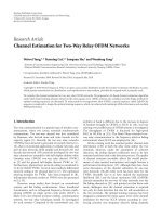
2 EURASIP Journal on Advances in Signal Processing
Audio mono 11.025 Hz
Onset-energy function
Reassigned sp ectrogram
Log-scale
Threshold >
50 dB
Low-pass filter
High-pass filter (diff)

Half-wave rectification
Sum over frequencies
Temp o d e te c t io n
Instantaneous periodicity
DFT ACF
FM-ACF
Combined DFT FM-ACF
Temp o s ta t e s
-Tempo
- Meter/beat subdivision
Viterbi decoding
Beat marking
PSOLA-based marking
Figure 1: Flowchart of our system for tempo, meter estimation, and beat marking.
mapped auto-correlation function is proposed which allows a
better discrimination between various existing periodicities
(tatum, tactus, measure). A Viterbi decoding algorithm then
estimates simultaneously the most likely tempo and meter
over time using proposed meter/beat subdivision templates.
The system is noncausal (therefore non real-time) since it
uses information from future events (through the length of
the analysis window and the use of a Viterbi algorithm). The
flowchart of the system is represented in Figure 1.
Numerous studies exist concerning tempo and beat esti-
mation. We refer the reader to [4] for a recent report on state-
of-the-art tempo estimation algorithms. Using the taxonomy
proposed in [4], we briefly review current directions in order
to locate our algorithm in the field. Tempo estimation algo-
rithms can first be distinguished from the analyzed materials:
symbolic data [5, 6] or audio data. Algorithms based on au-

dio analysis usually start by a front-end which either plays
the role of an “audio-to-symbolic” translator (extract the ex-
act location of the onsets of the events) [7–11]orextracts
frame-based audio features such as energy, energy variations,
energy in subbands or chord changes [2, 12, 13]. In the lat-
ter case, the features should represent significant cues con-
cerning the presence of musical events and (or) their roles in
the metrical structure. Depending on the kind of informa-
tion provided by this front-end and the context of the ap-
plication (real-time beat tracking or offline tempo estima-
tion), a large variety of processes are used to track/estimate
the tempo. In the case of a sequence of onsets, time interval
histograms (inter-onset-histogram [8, 14]) are often used to
detect the main periodicities. In the case of frame-based fea-
tures, a periodicity measure (Fourier transform, autocorre-
lation function, narrowed-ACF [15], wavelets, comb filter-
bank) is mostly used. The periodicity measure can be used to
estimate directly the tempo or to ser ve as observation for the
estimation of the whole metrical structure through (proba-
bilistic) models: estimation of the tatum, tactus (beat), mea-
sure and (or) estimation of systematic time deviations such
as the swing fac tor [2, 11, 16, 17].
Paper organization
The paper is organized as follows. In Section 2,wepresent
the front-end of our system for the extraction of the onset-
energy function based on a proposed reassigned spectr al en-
ergy flux. This onset-energy function is then used to estimate
the dominant periodicities at each t ime. In Section 3.1,we
present a new periodicity measure based on a combination
of discrete Fourier transform and frequency-mapped auto-

correlation function. In Section 3.2, we present our proba-
bilistic model of tempo, the meter/beat subdivision templates
and the Viterbi decoding algorithm which allows the estima-
tion of the most likely tempo and meter path over time. In
Section 4, we evaluate the performances of our system on
four different test sets among which three were used during
the ISMIR 2004 tempo induction contest.
2. ONSET-ENERGY FUNCTION
In order to detect the tempo of a piece of music from an
audio signal, one needs first to extract meaningful informa-
tion in terms of musical periodicit y from the signal. This
is the goal of the front-end of any audio-based tempo esti-
mation algorithm. Front-ends can perform onset detection.
However, by experimenting with this approach, we found
it unreliable considering the consequences that false posi-
tive and false negative detections can have on the subsequent
stages of the tempo estimation process. In [18] it has also
been found that algorithms based on onset detection suffer
more from distortion of the signal than the ones based on
frame features.
1
In addition to that the concept of discrete
onsets remains unclear for a large class of sounds such as
slow attack, slow transition between notes without an attack
phase and slow transition between chords such as played by
1
Note however that [14]arguesthataweakonsetdetectorissuitablefor
tempo induction.
Geoffroy Peeters 3
a string section. When front-ends extract frame-based au-

dio features, the most commonly used features are the vari-
ation of the signal energy or its variation inside several fre-
quency bands [12]. Since our interest is not only in music
with percussion but also in music without percussion, our
function should also react to any musically meaningful vari-
ations such as note transitions at constant global energy or
slow attacks. These variations are usually visible in a spec-
trogram representation. Reference [17] proposes a func tion,
called the spectral energy flux, which measures the varia-
tion of the spectrogram over time. For the computation of
the spectrogram, [17] uses a window of length about 10 ms.
This would lead according to [19] to a spectral resolution
2
of about 200 Hz. This spectral resolution is too large for
the detection of t ransitions between adjacent notes especially
in the lowest frequencies. In order to achieve such detec-
tion, one would need a much longer window, but then this
would be to the detriment of the temporal precision of on-
set locations. This is the usual time versus frequency reso-
lution trade-off. One would need a short window for accu-
rate temporal location of percussive onset and a long win-
dow for accurate detection of transition between adjacent
notes.
For this reason, we propose to compute the spectral en-
ergy flux using the reassigned spectrogram instead of the
normal spectrogram. By using phase information, the reas-
signed spectrogram allows significant improvement of tem-
poral and frequency resolution, therefore avoiding attacks
blurring and better differentiation of very close pitches. Be-
cause of that, we argue that using a single long window with

the reassigned spectrogram is suitable for onset detection for
both percussive and nonpercussive audio.
2.1. Reassigned spectrogram
In the following, we call “bin” a specific point of the short
time Fourier tra nsform grid defined by its frequency ω
k
and
time t
m
. The reassigned spectrogram [20] consists of reallo-
cating the energy of the “bins” of the spectrogram to the fre-
quency ω
r
and time t
r
corresponding to their center of grav-
ity. It has already been used for applications such as transient
detection, glottal closure instant detection in speech, sinu-
soidality coefficient or harmonic frequency location [21–24].
The reassignment of the frequencies is based on the com-
putation of the instantaneous frequency which is the time
derivative of the phase. We note x the signal, h the analysis
window of length L centered on time t
m
, dh the time deriva-
tive of the window h(dh
= ∂h(t)/∂t), STFT
h
the short time
Fourier transform computed using h,andSTFT

dh
the one
computed using dh. The reassignment of the frequencies can
be efficiently computed by
ω
r

x, t
m
, ω
k

=
ω
k

STFT
dh

x, t
m
, ω
k

STFT
h

x, t
m
, ω

k


,(1)
where
stands for the imaginary part. The reassignment of
2
For two sinusoidal components of equal amplitude, the spectral resolu-
tion is the minimal distance between their frequencies that guarantee that
no overlap between their main lobe occurs above a
3 dB level. The spec-
tral resolution depends on the window length and shape.
4000
2000
0
Frequency (Hz)
1.52 2.533.54
Time (s)
(a)
Reas
92 ms
46 ms
23 ms
1.52 2.533.54
Time (s)
(b)
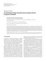
Figure 2: From top to bottom: (a) reassigned spectrogram com-
puted using a window length of 92.8 ms, superimposed: manually
annotated onset locations, (b1) corresponding reassigned spectral
energy flux function, (b2) normal spectral energy flux function

computed using a window length of 92 ms, (b3) 46 ms, (b4) 23 ms
on [signal: Asian Dub Foundation, RAFI, track 01 “Assassin” from
the “songs” database of the ISMIR 2004 test set].
the times is based on the computation of the group delay
which is the frequency derivative of the phase spectrum. We
note th the frequency derivative of the window h(th
= t h(t))
and STFT
th
the short time Fourier transform computed us-
ing th. The reassignment of the times can be efficiently com-
puted by
t
r

x, t
m
, ω
k

=
t
m
+ R

STFT
th

x, t
m

, ω
k

STFT
h

x; t
m
, ω
k


,(2)
where R stands for the real part.
Each “bin” (ω
k
, t
m
) of the spectrogram is then reassigned
to its center of gravity (ω
r
, t
r
) using (1)and(2). Since ω
r
and
t
r
are real-valued, we round them to the closest discrete fre-
quency ω

k
and discrete time t
m
of the STFT grid. The bins
are finally accumulated in the time and frequency plane.
2.2. Reassigned spectral energy flux
Except for the use of reassigned spectrogram, the computa-
tion of the reassigned spectral energy flux is close to the com-
putation of the normal spectral energy flux. It is done in the
following way.
(1) The signal is first down-sampled to 11.025 Hz and
converted to mono (mixing both channels).
(2) The reassigned spectrogram X(ω
k
, t
m
)iscomputed
using a hamming window. A long window of 92.8 ms (1023
samples) is used in order to achieve a good frequency reso-
lution. This favors the detection of note changes in the spec-
trum and therefore high values in the spectral flux. The de-
crease of the time resolution due to the use of a long w indow
is compensated by the use of the group delay (see Figure 2
4 EURASIP Journal on Advances in Signal Processing
4000
2000
0
Frequency (Hz)
00.511.522.533.54
Time (s)

(a)
Reas
92 ms
46 ms
23 ms
00.511.522.533.54
Time (s)
(b)
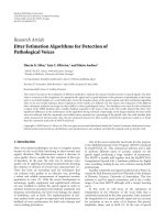
Figure 3: Same as Figure 2 but on [signal: Bernstein conducts
Stravinsky, track 23 “The jovial merchant with two gypsy girls”
from the “songs” database of the ISMIR 2004 test set].
and the corresponding discussion below). The number of
bins of the DFT used in (1)and(2) is 1024. The hop size
is set to 5.8 ms (64 samples).
(3) As in [7], the energy spectrum is converted to the
log scale. The use of the log scale will allow us in step (4)
to work on variations of energy relative to the energy level
since ∂ log(A(t))/∂t
= (∂A(t)/∂t)/A(t). A threshold of 50 dB
below the maximum energy is applied.
(4) The energy inside each frequency band e
log
(ω
k
, t
m
)is
low-pass filtered with an elliptic filter of order 5 and a cut-
off frequency of 10 Hz. The goal of the low-pass filter is to
avoid the detection of spurious onsets due to the presence

of background noise or noise events such as cymbal sounds.
The resulting energy signals are then differentiated using a
simple [1,
1] differentiator. The number of frequency bands
is among half the size of the DFT used in step (2), 500 in our
case.
(5) The resulting energy signals e
filter
(ω
k
, t
m
) are then
half-wave rectified. We note them e
HWR
(ω
k
, t
m
).
(6) For a specific time t
m
, the sum over all frequency
bands ω
k
is computed: e(t
m
) =

k

e
HWR
(ω
k
, t
m
). The result-
ing energy function e(n = t
m
) has a sampling rate of 172 Hz.
3
2.3. Comparison with the spectral energy flux
In Figures 2 and 3, we compare the reassigned and the nor-
malspectralenergyfluxfunctions.Thelatterhasbeenob-
tained by using the normal spectrogram instead of the re-
assigned spectrogram in step (2) of Section 2.2. Each figure
represents the reassigned spectrogram using a window of
3
Note that one could easily derive the onset locations by applying a thresh-
old on e(n).
length 92.8 ms, the corresponding reassigned spectral en-
ergy flux function, noted e
reas
(n), and three versions of
the normal spectral energy flux functions computed using
three different window lengths for the spectrogram (92.8ms,
46.3ms and 23.1ms), noted e
92
(n), e
46

(n), and e
23
(n), re-
spectively. Figure 2 represents the results for percussive audio
(rock music) and Figure 3 for nonpercussive audio (classi-
cal music). In the case of percussive audio, we have super-
imposed the manual annotation of the onset locations to
the reassigned spectrogram. In Figure 2, it can be seen that
many of the percussive onsets visible in e
reas
(n) are missing
in e
92
(n). This comes from the blurring that occurs on the
normal spectrogram due to the use of a long window. In this
case, a shorter window is needed in order to highlight the on-
sets in e(n) as the one used for e
23
(n). In Figure 3,weobserve
the inverse behavior. Many onsets visible in e
reas
(n) are miss-
ing in e
23
(n). This comes from the weak frequency resolution
obtained using a short window. In this case, a longer window
is needed in order to highlight the onsets in e(n), as the one
used for e
92
(n). In the case of the spectrogram, both types of

signal would thus require a different window length. We see
that with a single window length, the reassigned spectrogram
succeeded to highlight the onsets in both cases.
We continue this comparison in Section 4.3.1 where we
evaluate the influence of the choice of the reassigned or nor-
mal spectral energy flux function as well as the influence of
the window length on the global tempo recognition rate.
3. TEMPO DETECTION
We estimate the tempo from the analysis of the onset-energy
function e(n). The algorithm we propose works in two stages:
(i) first we estimate the dominant periodicities at each time
(Section 3.1); (ii) then we estimate the tempo, meter, and
beat subdivision paths that best explain the observed peri-
odicities over time (Section 3.2).
3.1. Periodicity estimation
Periodicity estimation of a signal is often done using discrete
Fourier transform (DFT) or autocorrelation function (ACF).
Ideally , e(n) is a periodic signal that can be roughly modeled
as a pulse train convolved with a low-pass envelope. If we
note f
= f
0
for fundamental frequency, the outcome of its
DFT is a set of harmonically related frequencies f
h
= hf
0
.
Depending on their relative amplitude it can be difficult to
decide wh ich harmonic corresponds to the tempo frequency.

If we note τ = 1/f
0
the period of e(n), the outcome of its
ACF is a set of periodically related lags τ
h
= h/ f
0
. Here also
it can be difficult to decide which period corresponds to the
tempo lag . Algorithms like the two-way mismatch [8, 25]or
maximum likelihood [ 26 ] try to solve this problem. In [27]
we have proposed a more straightforward approach that we
apply here to the problem of tempo periodicity estimation.
3.1.1. Combined DFT and frequency-mapped ACF
The octave uncer tainties of the DFT and ACF occur in in-
verse domains: frequency domain f
h
= hf
0
for the DFT, lag
domain τ
h
= h/ f
0
, or inverse frequency domain f
h
= f
0
/h
for the ACF. We use this property to construct a combined

Geoffroy Peeters 5
1
0
1
012 345 67
Time (s)
Signal
(a)
1
0.5
0
012345678910
Frequency (Hz)
Amplitude DFT
(b)
1
0.5
0
012345678910
Frequency (Hz)
Amplitude interpolated FM-ACF
(c)
1
0.5
0
012345678910
Frequency (Hz)
Amplitude DFT/FM-ACF
(d)
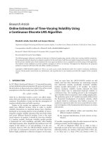
Figure 4: Simple example of combination between the DFT and the

ACF. From top to bottom: (a) sig nal, (b) magnitude of the DFT, (c)
ACF function mapped to the frequency domain, (d) product of (b)
and (c); on [signal: periodic impulse signal at 2 Hz].
function that reduces these uncertainties. We believe this
combined function can be very useful for the detection of
the various periodicities of a rhythm since it allows to better
discriminate the various periodicities of the measure, tactus,
and tatum (see Figure 6 in the remaining).
Example 1. In Figure 4, we illustrate the principle of the
method with a simple example. Figure 4(a) represents a peri-
odic impulse signal at 2 Hz, Figure 4(b) its DFT, Figure 4(c)
its ACF mapped to the frequency domain (the lags τ
l
are rep-
resented as frequencies f
l
= 1/τ
l
), Figure 4(d) the product of
the DFT and this frequency-mapped ACF. Only the compo-
nent at f = f
0
remains.
4
4
In this example, we rely on the fact that energy exists in the DFT at the
frequency f
= f
0
. In order to solve a possible “missing fundamental”

(no energy at f
= f
0
), we have proposed in [27] the use of the auto-
correlation of the DFT instead of the use of the direct DFT. In this paper,
we will ho wever use the direct DFT.
1
0.5
0
0.5
1
Amplitude
012345678910
Frequency (Hz)
DFT
Cosine at τ
= T
0
/2
f
= 2 f
0
Cosine at τ = T
0
f = f
0
Cosine at τ = 2T
0
f = f
0

/2
(a)
1
0.5
0
0.5
1
Amplitude
00.511.522.533.544.55
Lag (s)
ACF
τ
= T
0
/2
τ
= T
0
τ = 2T
0
(b)
Figure 5: (a) magnitude of the DFT of the signal; superimposed:
cosine at τ
= T
0
/2, T
0
,2T
0
and f = 2 f

0
, f
0
, f
0
/2 positions; (b) au-
tocorrelation function; superimposed: τ
= T
0
/2, T
0
,2T
0
positions;
on [signal: periodic impulse signal at 2 Hz].
Explanations
This interesting property comes f rom the fact that the ACF
r(τ) of a signal is equal to the inverse Fourier transform of
its power spectrum
S(ω)
2
. Since the power spectrum is real
and symmetric, its (inverse) Fourier transform reduces to the
real part. Therefore,
r(τ) can be considered as the projection
of S(ω)
2
on a set of cosine functions g
τ
(ω) = cos(ωτ)with

frequencies equal to the lag τ. In other words, r(τ)measures
the periodicity of the peak positions of the power spectrum.
Example 2. In Figure 5, we illustrate this for a periodic im-
pulse signal at f
0
= 2 Hz. We decompose g
τ
(ω) into its posi-
tive and negative parts: g
τ
(ω) = g
+
τ
(ω) g
τ
(ω). Positive val-
ues of
r(τ) occur only when the contribution of the projec-
tion of S(ω)
2
on g
+
τ
(ω) is greater than the one on g
τ
(ω)
(this is the case for the subharmonics of f
0
, τ = k/ f
0

, k N
+
in the figure); nonpositive values when the contribution of
g
τ
(ω) is larger than or equal to the one of g
+
τ
(ω) (this is
the case for the higher harmonics of f
0
, τ = 1/(kf
0
), k>1,
k N
+
in the figure). It is easy to see that only for the value
τ
= 1/f
0
we have simultaneously a maximum of the projec-
tion of
S(ω)
2
on g
τ
(ω) and a peak of energy in S(ω)
2
at
f = 1/τ.

This inverse octave uncertainty of the DFT and ACF is
used to compute our new periodicity measure as follows.
6 EURASIP Journal on Advances in Signal Processing
0.6
0.4
0.2
0
0.6
0.4
0.2
0
0.6
0.4
0.2
0
0.6
0.4
0.2
0
0 100 200 300 400 500
Frequency (bpm)
Duple/simple
Duple/compound
Triple/simple
Triple/compound
1/3
1/2
1
234
(a)

1
5
0
1
5
0
1
5
0
1
5
0
0123
Time (s)
(b)
Figure 6: (a) Metrical patterns of the combined DFT/FM-ACF for a tempo of 120 bpm and various theoretical typical rhythms; (b) corre-
sponding temporal signals.
Computation
We first make e(n) a zero-mean unit-variance signal. e(n)is
then analyzed both by the following.
(1) DFT:wenoteS(ω
k
, t
m
) the magnitude spectrum of
e(n)forafrequencyω
k
andaframecenteredaroundtimet
m
.

A hamming window is used with length equal to 8 s. The hop
size is set to 0.5s.
(2) Frequency mapped ACF (FM-ACF):wenote
r(τ
l
, t
m
)
the autocorrelation function of e(n)foralagτ
l
and a frame
centered around time t
m
. This function is normalized in
length and in maximum value. The normalized-in-length
autocorrelation function is defined as
r(l, m)
=
1
L l
L l 1

n=0
e

n + m
L
2

e


n + l + m
L
2

,(3)
where l is the lag τ
l
expressed in samples, m the time of the
frame t
m
in samples, and L the window length in samples.
The normalization in maximum value (at the zeroth-lag) is
obtained by r(l) = r(l)/r(0). A rectangular window is used
with length equal to 8 s. The hop size is set to 0.5s.
The value
r(τ
l
, t
m
) represents the amount of periodicity
of the signal at the lag τ
l
or at the frequency ω
l
= (2π)/τ
l
for
all l>0. Each lag τ
l

is therefore “mapped” in the frequency
domain. Of course since r(τ
l
, t
m
) has a constant resolution
in lag,
r(ω
l
, t
m
) has a decreasing resolution in frequency. In
order to get the same linearly spaced frequencies ω
k
as for
the DFT, we interpolate
5
r(τ
l
, t
m
) and sample it at the lags
τ
l
= (2π)/ω
k
. For this computation, we only consider the
frequencies ω
k
corresponding to tempo values between 30

and 600 bpm (ω
k
[0.5, 10] Hz, τ
l
[0.1, 2] s). Final ly,
5
Note that this does not improve the frequency resolution of r.
half-wave rectification is applied to r(ω
k
, t
m
)inordertocon-
sider only positive auto-correlation.
(3) Combined function: the DFT and the FM-ACF pro-
vide two measures of periodicity at the same frequencies ω
k
.
We finally compute a combined function Y(ω
k
, t
m
)bymul-
tiplying the DFT and the FM-ACF at each frequency ω
k
:
Y

ω
k
, t

m

= S

ω
k
, t
m

r

ω
k
, t
m

. (4)
In the following Y(ω
k
, t
m
) will be considered as our signal
observation.
Choice of a window length
The length of the window used for the computation of the
DFT and the ACF affects the interpretation one can make
concerning the observed periodicities. Short windows tend
to capture tatum periodicity, middle ones tactus periodic-
ity, and long ones periodicity of the measure. For a 120 bpm
musical piece, the length of a beat period is 0.5s. In order

to discriminate the beat frequencies in a spectrum (to avoid
spectral leakage), one would need a length larger than 2 s (4
time the period length). Also, in order to observe the period-
icity of the measure this would lead to 8 s for a 4/4 meter, our
choice for the system. We also apply a zero-padding factor
of 4.
6
The number of frequencies ω
k
of the DFT is therefore
equal to 8192 bins
7
and the distance between two f requencies
is equal to 1.26 bpm (0, 021 Hz). The hop size is set to 0.5s.
In the left part of Figure 6, we represent the patterns of
Y(ω
k
) for various theoretical ty pical rhythm characteristics
6
The number of bins of the DFT is taken as 4 times the smallest power of
two that is greater than or equal to the window length.
7
Note however that we only consider the frequencies corresponding to
tempo values between 30 and 600 bpm.
Geoffroy Peeters 7
2
1
0
Amplitude
0 50 100 150 200 250 300 350 400

Frequency (bpm)
DFT/FM-ACF
DFT
1/31/21 2 3
(a)
2
1
0
Amplitude
0 20 40 60 80 100 120 140 160
Frequency (bpm)
DFT/FM-ACF
DFT
1/31/21 2 3
(b)
2
1
0
Amplitude
0 100 200 300 400 500 600
Frequency (bpm)
DFT/FM-ACF
DFT
1/31/21 2 3
(c)
Figure 7: Comparison between the DFT (thin line) and the
combined DFT/FM-ACF (thick line) measured on real signals:
(a) quadruple/simple meter, (b) duple/compound meter, (c)
triple/simple meter. Superimposed: ground-truth tempo (1), 1/2
and 2 time the tempo, 1/3 and 3 time the tempo.

and a tempo of 120 bpm: duple/simple meter (eighth note
at 2/4), duple/compound meter (6/8), triple/simple meter
(eighth note at 3/4), triple/compound meter (9/8). In the
upper part of the figure the integer number 1 refers to the
tactus, the highest peak to the right (2 or 3) is the tatum
and the highest peak to the left (1/2or1/3) to the mea-
sure level. The resulting patterns of Y(ω
k
) are simple. This
comes from the fact that Y(ω
k
)istheproductoftwoin-
verse periodic series based on the periodicity of the measure
(kf
m
) and of the tatum ( f
t
/k ). Figure 6(b) represents the
corresponding temporal signal. The tactus period is equal to
0.5s.
In Figure 7, we compare the mean values over time of
S(ω
k
, t
m
)andY(ω
k
, t
m
), noted S(ω

k
)andY(ω
k
), measured
on real signals. The signal represented in Figure 7(a) is a
quadruple/simple meter.
8
Remark the large difference be-
tween the values taken by
S(ω
k
)andY(ω
k
). The value at
the tempo frequency (1) is much more emphasized in
Y(ω
k
)
than in
S(ω
k
). Figure 7(b) represents a duple/compound
8
Enya, Watermark, “Orinoco flow,” [Rhino/Warner Bros].
meter.
9
As in Figure 6, we observe the typical 1, 3 pattern
in
Y(ω
k

). Figure 7(c) represents a triple/simple meter.
10
As
in Figure 6, we observe the typical 1/3, 1 pattern in
Y(ω
k
). In
all these cases,
Y(ω
k
) gives a better emphasis on the tempo
and rhythm specificities than
S(ω
k
).
3.2. Tempo estimation
The dominant periodicities Y(ω
k
, t
m
)areestimatedateach
time t
m
. As depicted in Figure 6, Y (ω
k
, t
m
)doesnotonlyde-
pend on the tempo (120 bpm in Figure 6) but also on the
characteristics of the rhythm, at least on the subdivision of

the meter and of the beat. We therefore look for the temporal
path of tempo and meter/beat subdivision that b est explains
Y(ω
k
, t
m
).
Tempo states
In the following we consider three different kinds of me-
ter/beat subdivisions, named meter/beat subdivision tem-
plates (MBST):
(i) the duple/simple (noted 22 in the following),
(ii) the duple/compound (noted 23, example is 6/8 meter)
and
(iii) the triple/simple (noted 32, example is 3/4 meter).
We define a “tempo state” as a specific combination of a
tempo frequency b
i
and an MBST m
j
: s
ij
= [b
i
, m
j
]with
i I the set of considered tempo and j 22, 23, 32 the
three considered MBSTs. We look for the most likely tem-
poral succession of “tempo states” given our observations.

We formulate this problem as a Viterbi decoding algorithm
[28].
11
Viterbi decoding algorithm
Viterbi decoding algorithm, as used in HMM decoding [29],
requires the definition of three probabilities: an emission
probability of the states p
emi
(Y(ω
k
, t
m
) s
ij
(t
m
)), a t ransi-
tion probability between two states p
t
(s
ij
(t
m+1
), s
kl
(t
m
)), and
a prior probability of each state p
prior

(s
ij
(t
0
)).
The emission probability p
emi
(Y(ω
k
, t
m
) s
ij
(t
m
)) is the
probability that the model emits a given signal observation
Y(ω
k
, t
m
)attimet
m
given that the model is in state s
ij
at
time t
m
. This probability could be learned from annotated
data as we did in [30].

12
In the present system, we use a more
straightforward computation based on the theoretical metri-
cal patterns represented in Figure 6.Foraspecifictempob
i
and MBST m
j
,wefirstcomputeascoredefinedasaweighted
9
Boyz II Men, Coolexhighharmony, “End of the road” [Motown].
10
Viennese Waltz “media104409” from the “ballroom-dancer” database of
the ISMIR 2004 test set.
11
Our method shares some similarities with [17] in the use of a dynamic
programming technique. Reference [17] uses it to estimate simultane-
ously the most likely tempo and downbeat location over time based on
the observation of the energy flux signal and considering only a du-
ple/simple meter. We use it here to estimate simultaneously the most likely
tempo and meter/beat subdivision over time based on the observation of
Y(ω
k
, t
m
).
12
It should be noted that in [31] a weighted sum of specific ACF periodici-
ties has also been proposed in a task of meter and tempo estimation.
8 EURASIP Journal on Advances in Signal Processing
sum of the values of Y(ω

k
, t
m
) at specific frequencies:
score
i, j

Y

ω
k
, t
m

=
5

r=1
α
j,r
Y

ω = β
r
b
i
, t
m

,(5)

where β
represents the various ratios of the considered
frequency ω to the tempo frequency b
i
of the state s
ij
,
β
=

1
3
,
1
2
,1,1.5, 2, 3

. (6)
These ratios correspond to significant frequency components
for the triple meter, duple meter, tempo, “penalty” (see be-
low), simple and compound meter. α
j
represents the weight-
ings of each of these components. These weightings depend
on the MBST m
j
of the state s
ij
and have been chosen to bet-
ter discriminate the various MBSTs:

α
22
= [ 1, 1, 1, 1, 1, 1] if m
j
= 22,
α
23
= [ 1, 1, 1, 1, 1, 1] if m
j
= 23,
α
32
= [1, 1, 1, 1, 1, 1] if m
j
= 32.
(7)
The ratio β
= 1.5 is called the “penalty” ratio. It is used
to reduce the confusion between 22 and 23/32 MBST. In-
deed, the eighth note frequency of a rhythm at x bpm in a 22
MBST (tactus at the quarter note) can be interpreted as the
eighth note triplet frequency of a rhythm at (2/3)x bpm i n a
23 MBST (tactus at the dotted quarter note).
13
The negative
weighting given to the ratio 1.5 penalizes these choices.
The probability that state s
ij
emits a given signal observa-
tion is based on this score and is computed as

p
emi

Y

ω
k
, t
m

s
ij

t
m

=
score
i, j

Y

ω
k
, t
m


i, j
score

i, j

Y

ω
k
, t
m

. (8)
The transition probability favors continuity of tempi and
MBST over time. We consider independence between tempo
and MBST.
14
We compute this probability as the product of a
tempo continuity probability and an MBST continuity prob-
ability,
p
t

s
ij

t
m+1

s
kl

t

m

=
p
t

b
i

t
m+1

b
k

t
m

p
t

m
j

t
m+1

m
l


t
m

.
(9)
The goal of the first probability is to favor continuous tempi.
We set it as a Gaussian pdf N
μ=b
k
,σ=5
(b
i
). The goal of the
second probability is to avoid MBST jumps from frame to
frame. We set it empirical ly to 0.0833 for j = l and 0.833 for
j
= l.
The prior probability p
prior
(s
ij
(t
0
)) is the prior probabil-
ity to observe a specific tempo i and a specific MBST j. This
probability is set according to musical knowledge. Assump-
tions about tempo range and meter can be made according
to the music genre of the track. This music genre could be
13
The same is true for the sixteenth note and a rhythm at (4/3)x bpm in a

23 MBST.
14
This is not exactly true since some joint tempo/meter transitions are more
likely than others.
400
300
200
100
Bpm
10 20 30 40 50 60 70
Time (s)
1
233
23
(a)
3–2
2–3
2–2
Meter
0 50 100 150
Time (s)
(b)
Figure 8: (a) tempo estimation over time (b) MBST estimation
over time; on [signal: “Standard of excellence-accompaniment CD-
Book2-All inst 88. Looby Loo”].
automatically estimated by including a front-end for music
genre recognition in our system. Since our current system
does not include such a front-end, we simply favor the de-
tection of tempo in the range 50–150 bpm but we do not
favor any MBST in particular. We set it as a Gaussian pdf:

p
prior
(s
ij
(t
0
)) = p
prior
(b
i
(t
0
)) = N
μ=120,σ=80
(b
i
).
A standard Viterbi decoding algorithm is then used to
find the best path of states [b
i
, m
j
] over time, which gives
us simultaneously the best tempo and MBST path that ex-
plain Y(ω
k
, t
m
). Finally, in order to increase the precision of
the tempo estimation, frequency interpolation is performed

around the value Y(b(t
m
), t
m
). For this a second-order poly-
nomial, p(ω) = aω
2
+bω+c, is fitted to the values of Y(ω
k
, t
m
)
around ω
k
= b(t
m
). The value corresponding to the maxi-
mum of the polynomial, ω
max
= b/(2a), is chosen as the
final tempo value.
Example 3. In Figure 8 we illustrate the estimation of time-
varying MBST. Figure 8(a) represents the estimated tempo
track over time (indicated with “+”s around 100 bpm) super-
imposed to the periodicity observation Y(ω
k
, t
m
)represented
as a matrix and annotated by hand (1 for tactus frequency, 2

and 3 for tatum frequency). Figure 8(b) represents the esti-
mated MBST over time. The system has estimated a constant
tempo during the entire track duration but depending on the
local periodicities (1 and 3 or 1 and 2), the MBST is esti-
mated as either 23 or 22. Both tempo and MBST estimations
are correct.
Example 4. In Figure 9, we illustrate the estimation of time-
varying tempo on Brahms “Ungarische Tanze n5.”
15
This
15
The t rack has been annotated by hand into beat locations. The local
tempo has then been derived from the distance between adjacent beats.
Note that the resulting tempo would not necessarily correspond to the
perceived tempo.
Geoffroy Peeters 9
250
200
150
100
50
Bpm
20 40 60 80 100 120
Time (s)
Estimated tempo
Ground-truth tempo
Figure 9: Tempo estimation over time: estimated tempo (dashed
line), ground-truth tempo (continuous thick line) on [signal:
Brahms “Ungarische Tanze n5”].
piece is interesting since it has many quick tempo varia-

tions. The dashed thin line represents the estimated tempo
track while the continuous thick line represents the refer-
ence tempo. Both are superimposed to the observations ma-
trix Y(ω
k
, t
m
). The tempo has been estimated as twice the
reference tempo during the periods [0, 25], [ 34, 37], [58, 67],
[88, 101], and [110, 113] s and as half during the p eriod
[75, 85] s. The transitions being very quick in this part, the
algorithm decided there was a higher probability to remain
at 65 bpm.
4. EVALUATION
In this section, we evaluate the performances of our tempo
estimation system.
4.1. Test sets
Evaluation of algorithms is often done on personal test sets.
However, this makes the comparison with existing technolo-
gies hard. For this reason, and because of availability, we used
the three test sets of the ISMIR 2004 tempo induction contest
(see [18] for details). We also added a fourth “personal” test
set in order to represent also commercial radio music. The
test sets are
(i) the “ballroom-dancer” database:
16
698 tracks of 30 s
long. The following music genres are covered: cha cha, jive,
quickstep, rumba, samba, tango, Viennese waltz and slow
waltz music. The tracks are mainly in 4/4 and 3/4 meters and

with almost constant tempo except for the slow waltz music,
(ii) the “songs” database: 465 tracks of 20 s long. The
following music genres are covered: rock, classical, electron-
ica, latin, samba, jazz, afrobeat, flamenco, Balkan and Greek
16
.
Table 1: Comparison between reassigned and normal spectral en-
ergy flux for vari ous window lengths in a task of tempo estimation.
11.5ms 23, 1 ms 46, 3 ms 92, 8 ms
Acc1 Acc2 Acc1 Acc2 Acc1 Acc2 Acc1 Acc2
RSEF 48, 0 79, 4 49, 5 82, 4 49, 9 83, 2 49, 5 83,7
SEF
49, 7 80, 4 49,5 82, 6 49, 3 82, 8 49, 7 82, 2
music.Thetracksareinvariousmetersandwithconstantor
time variable tempo (flamenco, classical),
(iii) the “loops” database: 1889 tracks of “loops” to be
used in DJ sessions from the Tape Gallery.
17
Although the
database used in [18] had 2036 items, we had only a ccess to
1889 of them (92.8%). Also we had to manually correct part
of the annotations since some of them did not represent any
musical meaningful periodicities. When comparing our re-
sults with the ISMIR 2004 results, one should keep that in
mind. It is also worth to mention that, despite of its name,
the database contains a large part of non drum-loops sounds
like machine/engine noises with unclear periodicity,
(iv) the “poprock” database: 153 tracks of 20 s covering
commercial radio music from the last decades (80’s, 90’s,
00’s, including pop, rock, rap, musical comedy).

In the following, the results obtained with our system will
be compared with the ones obtained during the ISMIR 2004
tempo induction contest published in [18]. Each item of the
four test sets has been annotated by its mean tempo over
time. The “ballroom-dancer” and “poprock” databases have
also been annotated by the author in meter. We have used the
three following meters: 22 (if the annotated beats can be mu-
sically grouped by 2 and subdivided by 2), 23 (grouped by 2
divided by 3), 32 (grouped by 3 divided by 2).
The tracklist of the “poprock” database, as well as the
used tempo and meter annotations for the four test sets can
be found on the author’s web site.
18
4.2. Evaluation method
The tempo over time was extracted with our algorithm. The
tempo was not considered constant during the track dura-
tion. For each track, we compare the median value of the es-
timated tempo over time w ith the annotated tempo. As in
[18], we consider two accuracy measures:
(i) accuracy 1: percentage of tempo estimates within 4%
of the ground-truth tempo,
(ii) accuracy 2: percentage of tempo estimates within 4%
of either the ground-truth tempo, 1/2, 2, 1/3 or 3 the ground-
truth tempo. This allows taking into account the fact that var-
ious periodic levels often coexist within a given metric. Be-
cause the ground-truth meter is available for the “ballroom-
dancer” and “poprock” databases, we also indicate a more
restrictive definition of accuracy 2 that only considers the es-
timated tempo as correct when it is 1/2, 1 or 2 for the 22
meter, 1/3,1or2for32meter,1/2,1or3for23meter.

17
nd-effects-library.com.
18
peeters/eurasipbeat/.
10 EURASIP Journal on Advances in Signal Processing
Table 2: Results of the tempo estimation evaluation.
Ballroom Songs Loops Poprock
Acc1 Acc2 Acc1 Acc2 Acc1 Acc2 Acc1 Acc2
Time variable
22/23/32
65, 2 93, 1 49, 5 83, 7 56,1 80, 7 87, 6 97, 4
(89, 0) (97, 4)
Constant 22 68, 7 96, 9 39, 4 85, 2 59, 8 83, 1 81, 7 99, 4
ISMIR 2004 best 63, 2 92, 0 58, 5 91, 2 70, 7 81, 9
4.3. Results
4.3.1. Comparison between reassigned and normal
spectral energy flux
We first compare the results obtained using various choices
for the front-end of our system. We test the choice of the re-
assigned or normal spectral energy flux, noted RSEF and SEF,
respectively. In both cases, we test the influence of the win-
dow length, noted L. Four lengths are tested: L
= 11.5ms,
23.1ms,46.3 ms, and 92.2 ms. For this comparison, we only
use the “songs” database since this is the most balanced
database among the four, containing both percussive and
nonpercussive audio. In Tabl e 1, we indicate the accuracies 1
and 2 of the whole system for the eight versions of the front-
end. According to accuracy 1, all choices lead to close results
except for the choice of the RSEF with L

= 11.5ms which
has the lowest score. According to accuracy 2, the RSEF with
L
= 92.8 ms slightly outperforms the other methods.
19
This
therefore confirms the choice we have made previously. It is
interesting to consider that also for L = 46.3 ms, the RSEF
slightly outperforms the SEF. For both RSEF and SEF, the
lowest score is obtained with L = 11.5 ms, the choice made
in [17].
The results presented in the following are obtained with
the reassigned spectral energy flux and a window of length
92.6ms.
4.3.2. Evaluation of the system
In Table 2, we compare the results obtained using our sys-
tem (“time variable 22/23/32” row) with the best results ob-
tained during the ISMIR 2004 tempo induction contest (“IS-
MIR 2004 best” row). We indicate the accuracies 1 and 2 for
the four test sets. The values in parentheses correspond to the
restrictive accuracy 2.
In Figures 10, 11, 12,and13 we present detailed results
for each database. We define r as the ratio between the esti-
mated tempo and the ground truth tempo. The upper part
of each figure (a) represent the histogram of the values r in
log-scale over all instances of each database. The vertical lines
represent the values of r corresponding to usual tempo con-
fusions: 1/3, 1/2, 2/3, 4/3, 2, 3 (
1.58, 1, 0.58, 0.41, 1, 1.58
in log-scale). The lower part of each figure (b) indicates the

influence of the precision window width on the recognition
rate. The vertical line represents the precision window width
of 4% used in Table 2.
19
Since the database contains 465 titles, a difference of 0.21% indicates a
difference of one correct recognition.
For the “ballroom-dancer” database, the results are
65.2%/93.1% (89.0) which improve upon those obtained in
ISMIR 2004 (63.2%/92.0%). Considering accuracy 1, most
errors occurred in the jive and quickstep (half the tempo),
rumba (twice the tempo) and both waltzes. The jive and
quickstep explains the large peak at r
= 1/2 in the histogr am
of Figure 10. Considering accuracy 2, most errors occurred
in the slow waltz (the concept of onsets is unclear in the
slow chord transitions). We also evaluate the recognition rate
of the ground-truth meter. Comparing the estimated meter
with the ground-truth meter makes sense only for track with
correctly estimated tempo.
20
The recognition rate of meter
(for the 65.2% remaining tracks) is 88.7% for the 22 meter
(3.8% recognized as 23, 7.4% as 32), 43.9% for the 32 me-
ter (51.6% recognized as 22, 4.4% as 23). This is surprisingly
low.
For the “songs” database, the results are 49.5%/83.7%
which is lower than those obtained in ISMIR 2004 (58.5%/
91.2%) but would be the second best algorithm according to
accuracy 2. The large difference between accuracies 1 and 2
(and the high peak in the histogram of Figure 11 at r = 2) in-

dicates that in many cases the algorithm estimated the tatum
periodicity. Despite our 1.5penaltycoefficient, a secondary
peak exists in the histogram at r = 2/3 (detection of the
dotted quarter note). According to Figure 11, increasing the
width of the precision window to more than 4% would in-
crease a lot accuracy 2.
For the “loops” database, the results are 56.1%/80.7%,
just below those obtained in ISMIR 2004 (70.7%/81.9%) but
would be the second/third best algorithm. Three peaks exist
in the histogram at r
= 0.5, r = 2, and r = 4/3.
For the “poprock” database, the results are 87.6%/97.4%
(97.4%). The recognition rate of meter (for the 87.6% cor-
rectly estimated tempo) is 89.3% for the 22 meter (3% rec-
ognized as 23, 7.6% as 32), 100% for the 23 meter.
In order to check the importance of the meter/beat sub-
division and the time-varying estimation (Viterbi decod-
ing) parts of our algorithm, we have done the evaluation
again with a constant tempo and a 22 meter/beat subdivi-
sion hypothesis. For this, we only estimate the most likely
p
emi
(Y(ω
k
) [b
i
, 22]) of (8) and only using an average ob-
servation over time
Y(ω
k

). In this case, the weightings of (7)
are defined as α = [0,1,1,0,1,0], that is, we did not use
any penalty weightings. The results are indicated in Table 2
(“Constant 22” row).
Surprisingly, for the ballroom-dancer database, both ac-
curacies increase by about 3.5%. In this case, the evaluation
20
A track with a 32 meter will not be estimated as 32 if the estimated tempo
is twice the ground-truth tempo.
Geoffroy Peeters 11
400
300
200
100
0
Histogram
2 10 1 2
Log 2 (estimated tempo/correct tempo)
1/3
1/2
2/3
1
4/3
2
3
(a)
100
80
60
40

20
0
Accuracy 1/2
0 5 10 15 20
Precision window width
Accuracy 1
Accuracy 2
(b)
Figure 10: (a) Histogram of the ratios in log-scale between es-
timated tempi and correct tempi; (b) accuracy versus precision
window width (in (%) of correct tempo) for the ballroom-dancer
database.
of MBST has a negative effect on the result. For the songs
database, accuracy 1 decreases by almost 10% while accuracy
2 increases by 1.5%. The evaluation of MBST has therefore a
positive impact on accuracy 1, that is, it allows avoiding con-
fusion between the various levels of the metrical st ructure.
For the loops database, both accuracies increase by about 3%.
This is normal since the given hypothesis (constant tempo
and duple/simple meter) is largely valid for this database. It is
interesting to note that the simplified algorithm now outper-
forms in accuracy 2 (83.1%) the best results of ISMIR 2004
(81.9%). For the poprock database, accuracy 1 decreases by
6% while accuracy 2 increases by 2%. Here a lso, the evalua-
tion of MBST has a positive impact on accuracy 1.
200
150
100
50
0

Histogram
2 10 1 2
Log 2 (estimated tempo/correct tempo)
(a)
100
80
60
40
20
0
Accuracy 1/2
0 5 10 15 20
Precision window width
Accuracy 1
Accuracy 2
(b)
Figure 11: Same as Figure 10 for the songs database.
As a conclusion, when given no prior knowledge about
tempo evolution over time and meter/beat subdivision, the
use of the proposed MBST increases accuracy 1 (except
for the ballroom-dancer) and slightly decreases accuracy 2.
When constant tempo and duple/simple meter hypothesis
holds, the use of MBST has a negative effect.
CONCLUSION AND DISCUSSIONS
The system presented in this paper yields very good perfor-
mance for tempo estimation for a large variety of music gen-
res. Among the three test sets used for the ISMIR 2004 tempo
induction contest, our system outperformed once the previ-
ous best results and was close to them for the two others.
However, the automatic estimation of the meter, based on

the proposed meter/beat subdivision templates, remains un-
reliable.
12 EURASIP Journal on Advances in Signal Processing
1200
1000
800
600
400
200
0
Histogram
2 10 12
Log 2 (estimated tempo/correct tempo)
(a)
100
80
60
40
20
0
Accuracy 1/2
0 5 10 15 20
Precision window width
Accuracy 1
Accuracy 2
(b)
Figure 12: Same as Figure 10 for the loops database.
Try ing to improve our system, we should distinguish
two main problems. The first one concerns the extraction
of significant information from the audio signal that allows

the estimation of a musical periodicity. For this, we have
shown in an experiment that the proposed reassigned spec-
tral energy flux using a long analysis window can provide
slight improvement over the usual spectral energy flux es-
pecially for nonpercussive audio. We also base this asser-
tion on the first place obtained by our system in the non-
percussive audio category of the MIREX 2005 tempo con-
test.
21
However, the sole information extracted from the sig-
nal is related to energy (energy variations). This information
is surely too poor for the characterization of rhythm [17]. In-
clusion of features such as pitch, relative frequency positions,
21
Tempo Extraction
for details.
120
100
80
60
40
20
0
Histogram
2 10 1 2
Log 2 (estimated tempo/correct tempo)
(a)
100
80
60

40
20
0
Accuracy 1/2
0 5 10 15 20
Precision window width
Accuracy 1
Accuracy 2
(b)
Figure 13: Same as Figure 10 for the poprock database.
spectr al centroid/spread [3] could certainly improve the per-
formances of our system.
The second problem concerns the estimation of the
tempo itself. Because the tempo has inherent ambiguities due
to the various possible interpretations of a metrical struc-
ture of a rhythm, we have proposed to estimate it jointly
with the measure and tatum periodicities through the use of
meter/beat subdivision templates. This was possible since the
proposed combined DFT/ FM-ACF allows a good discrim-
ination between the measure, tactus, and tatum periodici-
ties. Considering the performance of the tempo estimation,
we believe this approach is promising. However, considering
the performance of the estimated meters, there is space for
improvements. There are two reasons for that. The first rea-
son comes from the weighting used in the templates that are
based on theoretical templates. These templates only repre-
sent the variety of possible existing rhythm patterns partially.
One solution would be to learn the templates from annotated
Geoffroy Peeters 13
data as we did in [30]. In the current work, we did not want

to use this information from the test sets. The second reason
comes from signal processing. The interpolation used during
the mapping of the ACF to the frequency domain degrades
the resolution of the combined function in the low frequen-
cies (where the measure/bar frequency is located). The me-
ter subdivision estimation is therefore more difficult than the
beat subdivision estimation. Among the most problematic
rhythms (except those in exotic meters) are the ones with
accentuations on dotted quarter notes that are frequent in
bossa-nova or funk music. Specific templates should be de-
voted to that as well.
As represented in Figure 1, the system also contains a beat
marking algorithm which we did not discuss here since it
was not possible to evaluate because of the lack of annotated
databases for beat locations. For the same reason, the time-
varying charac teristics of our algorithm have only been indi-
rectly tested in the median-tempo evaluation. Ongoing work
will concentrate on these improvements and evaluations.
ACKNOWLEDGMENTS
Part of this work was conducted in the context of the Eu-
ropean IST project Semantic HIFI
22
[32]. The author would
like to thank three anonymous reviewers for useful and de-
tailed suggestions. Many thanks also to the people who have
collaborated to the ISMIR 2004 tempo induction contest and
made the test sets and annotations available. To my father.
REFERENCES
[1] J. Bilmes, “Timing is of the essence: perceptual and compu-
tational techniques for representing, learning, and reproduc-

ing expressive timing in percussive rhythm,” M.S. thesis, MIT,
Cambridge, Mass, USA, 1993.
[2] A. Klapuri, A. Eronen, and J. Astola, “Analysis of the meter of
acoustical musical signals,” IEEE Transactions on Audio, Speech
and Language Processing, vol. 14, no. 1, pp. 342–355, 2006.
[3] F. Gouyon, A computational approach to rhythm description,
Ph.D. thesis, Universitat Pompeu Fabra, Barcelona, Spain,
2005.
[4] F. Gouyon and S. Dixon, “A review of automatic rhythm de-
scription systems,” Computer Music Journal,vol.29,no.1,pp.
34–54, 2005.
[5] J. C. Brown, “Determination of the meter of musical scores by
autocorrelation,” Journal of the Acoustical Society of America,
vol. 94, no. 4, pp. 1953–1957, 1993.
[6] P. Allen and R. Dannenberg, “Tracking musical beats in real
time,” in Proceedings of the International Computer Music Con-
ference and International Computer Music Association, pp. 140–
143, San Francisco, Calif, USA, September 1990.
[7] A. Klapuri, “Sound onset detection by applying psychoacous-
tic knowledge,” in Proceedings of the IEEE International Con-
ference on Acoustics, Speech and Signal Processing (ICASSP ’99),
vol. 6, pp. 3089–3092, Phoenix, Ariz, USA, March 1999.
[8] F. Gouyon, P. Herrera, and P. Cano, “Pulse-dependent analyses
of percussive music,” in Proceedings of AES 22nd International
Conference on Virtual, Synthetic and Entertainment Audio,pp.
396–401, Espoo, Finland, June 2002.
[9] J. Bello, Towards the automated analysis of simple polyphonic
music: a knowledge based approach, Ph.D. thesis, Queen Mary
University of London, London, UK, 2003.
22

.
[10] C. Uhle and J. Herre, “Estimation of tempo, micro time and
time signature from percussive music,” in Proceedings of the 6th
International Conference on D igital Audio Effects (DAFx ’03),
pp. 84–89, London, UK, September 2003.
[11] M. Goto, “An audio-based real-time beat tracking system for
music with or without drum-sounds,” Journal of New Music
Research, vol. 30, no. 2, pp. 159–171, 2001.
[12] E. D. Scheirer, “Tempo and beat analysis of acoustic musical
signals,” Journal of the Acoustical Society of America, vol. 103,
no. 1, pp. 588–601, 1998.
[13] J. Paulus and A. Klapuri, “Measuring the similarity of rhyth-
mic patterns,” in Proceedings of the 3rd International Confer-
ence on Music Information Retrieval (ISMIR ’02), pp. 150–156,
Paris, France, October 2002.
[14] S. Dixon, “Automatic extraction of tempo and beat from ex-
pressive performances,” Journal of New Music Research, vol. 30,
no. 1, pp. 39–58, 2001.
[15] J. C. Brown and M. S. Puckette, “Calculation of a “narrowed”
autocorrelation function,” Journal of the Acoustical Society of
America, vol. 85, no. 4, pp. 1595–1601, 1989.
[16] F. Gouyon and P. Herrera, “Determination of the meter of
musical audio signals: seeking recurrences in beat segment
descriptors,” in Proceedings of the 114th Convention of Audio
Engineering Society (AES ’03), Amsterdam, The Netherlands,
March 2003.
[17] J. Laroche, “Efficient tempo and beat tracking in audio record-
ings,” Journal of the Audio Engineering Society, vol. 51, no. 4,
pp. 226–233, 2003.
[18] F. Gouyon, A. Klapuri, S. Dixon, et al., “An experimental com-

parison of audio tempo induction algorithms,” IEEE Transac-
tions on Speech and Audio Processing, vol. 14, no. 5, pp. 1832–
1844, 2006.
[19] F. J. Harris, “On the use of windows for harmonic analysis
with the discrete Fourier transform,” Proceedings of the IEEE,
vol. 66, no. 1, pp. 51–83, 1978.
[20] P. Flandrin, Time-Frequency/Time-Scale Analysis,Academic
Press, San Diego, Calif, USA, 1999.
[21] G. Peeters and X. Rodet, “Sinola: a new analysis/synthesis
using spectrum peak shape distortion, phase and reassigned
spectrum,” in Proceedings of the International Computer Music
Conference (ICMC ’99), pp. 153–156, Beijing, China, October
1999.
[22] G. Peeters, Mod
`
eles et mod
´
elisation du signal sonore adapt
´
es
`
asescaract
´
erist iques locales, Ph.D. thesis, Universit
´
e Paris VI,
Paris, France, 2001.
[23] A. R
¨
obel, “A new approach to transient processing in the phase

vocoder ,” in Proceedings of the 6th International Conference on
Dig ital Audio Effects (DAFx ’03), pp. 344–349, London, UK,
September 2003.
[24] S. Hainsworth and P. Wolfe, “Time-frequency reassignment
for music analysis,” in Proceedings of International Computer
Music Conference (ICMC ’01), pp. 14–17, La Habana, Cuba,
September 2001.
[25] R. Maher and J. Beauchamp, “Fundamental frequency estima-
tion of musical signals using a two-way mismatch procedure,”
Journal of the Acoustical Society of America, vol. 95, no. 4, pp.
2254–2263, 1994.
[26] B. Doval and X. Rodet, “Fundamental frequency estimation
and tracking using maximum likelihood harmonic matching
and HMMs,” in Proceedings of the IEEE International Confer-
ence on Acoustics, Speech and Signal Processing (ICASSP ’93),
vol. 1, pp. 221–224, Minneapolis, Minn, USA, April 1993.
[27] G. Peeters, “Music pitch representation by periodicity mea-
sures based on combined temporal and spectral representa-
tions,” in Proceedings of the IEEE International Conference on
Acoustics, Speech and Signal Processing (ICASSP ’06), pp. 53–
56, Toulouse, France, May 2006.
14 EURASIP Journal on Advances in Signal Processing
[28] A. Viterbi, “Error bounds for convolutional codes and an
asymptotically optimum decoding algorithm,” IEEE Transac-
tions on Information Theory, vol. 13, no. 2, pp. 260–269, 1967.
[29] L. R. Rabiner, “Tutorial on hidden Markov models and se-
lected applications in speech recognition,” Proceedings of the
IEEE, vol. 77, no. 2, pp. 257–286, 1989.
[30] G. Peeters, “Rhythm classification using spectral rhythm pat-
terns,” in Proceedings of the 6th International Conference on

Music Information Retrieval (ISMIR ’05), pp. 644–647, Lon-
don, UK, September 2005.
[31] S. Dixon, E. Pampalk, and G. Widmer, “Classification of dance
music by periodicity patterns.,” in Proceedings of the 4th In-
ternational Conference on Music Information Retrieval (ISMIR
’03), pp. 159–165, Baltimore, Md, USA, October 2003.
[32] H. Vinet, “The Semantic Hifi project,” in Proceedings of the In-
ternational Computer Music Conference (ICMC ’05), pp. 503–
506, Barcelona, Spain, September 2005.
Geoffroy Peeters was born in Leuven, Bel-
gium, in 1971. He received his M.S. degree
in electrical engineering from the Univer-
sit
´
e-Catholique of Louvain-la-Neuve, Bel-
gium, in 1995 and his Ph.D. degree in com-
puter science from the Universit
´
e Paris VI,
France, in 2001. During his Ph.D., he devel-
oped new signal processing algorithms for
speech and audio processing. Since 1999, he
works at IRCAM (Institute of Research and
Coordination in Acoustic and Music) in Paris, France. His current
research interests are in signal processing and pattern matching ap-
plied to audio and music indexing. He has developed new algo-
rithms for timbre description, sound classification, audio identifi-
cation, rhythm description, automatic music structure discovery,
and audio summary. He owns several patents in these fields and
received the ICMC Best Paper Award in 2003. He has also coor-

dinated indexing research activities for the Cuidad, Cuidado, and
Semantic HIFI European projects. He is the coauthor of the ISO
MPEG-7 audio standard.