Báo cáo hóa học: " Research Article Recognition of Planar Objects Using Multiresolution Analysis" pdf

Hindawi Publishing Corporation
EURASIP Journal on Advances in Signal Processing
Volume 2007, Article ID 70351, 9 pages
doi:10.1155/2007/70351
Research Article
Recognition of Planar Objects Using Multiresolution Analysis
Nazlı G
¨
uney and Ays¸ın Ert
¨
uz
¨
un
Department of Electrical and Electronics Engineering, Bo
¯
gazic¸i University, 34342 Bebek, Istanbul, Turkey
Received 29 August 2005; Revised 29 May 2006; Accepted 16 July 2006
Recommended by Antonio Ortega
By using affine-invariant shape descriptors, it is possible to recognize an unknown planar object from an image taken from an
arbitr ary view when standard view images of candidate objects exist in a database. In a previous study, an affine-invariant function
calculated from the wavelet coefficients of the object boundary has been proposed. In this work, the invariant is constructed from
the multiwavelet and (multi)scaling function coefficients of the boundary. Multiwavelets are known to have superior performance
compared to scalar wavelets in many areas of signal processing due to their simultaneous orthogonality, symmetry, and short sup-
port properties. Going from scalar wavelets to multiwavelets is challenging due to the increased dimensionalit y of multiwavelets.
This increased dimensionality is exploited to construct invariants with better performance when the multiwavelet “detail” coef-
ficients are available. However, with (multi)scaling function coefficients, which are more stable in the presence of noise, scalar
wavelets cannot be defeated.
Copyright © 2007 Hindawi Publishing Corporation. All rights reserved.
1. INTRODUCTION
Object recognition is one of the most difficult problems in
computer vision. However, if the problem definition includes

only planar objects, which are to be viewed from arbitrary di-
rections, it is possible to design recognition systems that have
satisfactory performances. When the depth of an object along
the line of sight is small compared to the viewing distance of
the camera, as its images are produced from different view-
points, it seems to be going through an affine transformation.
Thus, for recognition of planar objects, it suffices to find suit-
able affine invariants. These invariants are shape descriptors
that remain unchanged even when the viewing point of the
camera changes. Therefore, it may be said that object recog-
nition is a search for invariants [1].
Recognition techniques are classified according to how
the shape descriptors are calculated from the images of ob-
jects. One such classification is based on whether the bound-
ary or the region of the object is required. Region-based tech-
niques take into account the whole region in the image corre-
sponding to the object, whereas boundary-based techniques
analyze the object boundary. Analyzing only the boundary
is advantageous compared to the region-based techniques
in terms of computational complexity, since the amount of
data to be processed substantially diminishes. Yet another
classification to discriminate between the shape descriptors
is whether they are local or global. Local techniques, which
usually resort to higher-order derivatives, are very much af-
fected by the presence of noise [1]. Global techniques, on
the other hand, consider the w h ole data when calculating
the shape descriptors, and hence suffer from occlusion of the
object. Fourier descriptors in [2] and the wavelet-transform-
based methods [3–5], which are the subject of this paper, are
examples of boundary-based global techniques, since com-

putation of the transform coefficients requires all of the
boundary coordinates.
Among the wavelet-transform-based techniques, the
work by Khalil and Bayoumi [4] deserves further attention.
When calculating the affine-invariant shape descriptor, they
have used the biggest number of wavelet scales. The affine-
invariant function proposed in [4] uses 7–12 wavelet scales.
Different boundaries may have similar wavelet coefficients
at a particular scale, but not at all scales [4]. Thus, with
more scales used, the more accurate the representation of the
boundary becomes. A database of 20 airplane objects is used
to test the recognition performance of the affine-invariant
function. Uniformly distributed noise at 50 dB and 20 dB
signal-to-noise ratios (SNR) is added to the randomly affine-
transformed object boundaries [4, 6]. However, only one re-
alization of noise and one object view are not sufficient to
assess the performance of the invariant function proposed.
Besides, only one type of wavelet, the one in [7], has been
used in the simulations accompanied with an inadequate
analysis as to which wavelet scales should be chosen.
2 EURASIP Journal on Advances in Signal Processing
Multiwavelets, which are generalizations of wavelets,
have shown superior performance compared to wavelets in
such areas as image compression [8] and image denoising
[9, 10]. These application areas are related to object recog-
nition, for they, too, require compact and accurate represen-
tations. Thus, the affine-invariant function should also ben-
efit from using multiwavelet coefficients instead of wavelet
coefficients. Since coefficients at different scales are multi-
plied together when calculating the invariant function, the

undecimated (redundant) multiwavelet transform, which is
also translation invariant, is employed. In [11], where pla-
nar shapes are represented with the orthogonal multiwavelet
transform coefficients, the multiwavelets are shown to be
more promising than scalar wavelets in terms of accuracy of
representation.
In this work, the affine-invariant function in [4]iscon-
structed from (multi)wavelet and (multi)scaling function co-
efficients of the object boundary. Extensive simulations are
made with three object databases and hundred views for each
of the objects. Four wavelets, two combined sets of wavelets,
and six multiwavelets are tested. The approximation proper-
ties of the (multi)wavelets are shown to be the most signifi-
cant criterion when choosing either the transform coefficient
scales or the type of (multi)wavelet. Moreover, whether the
objects are smooth or contain detail affect the performance
of the invariant function.
The rest of the paper is organized as follows. Section 2
reviews the orthogonal multiwavelet transform and explains
the procedure for calculating the redundant multiwavelet
transform. The affine-invariant function in [4] is introduced
in Section 3, where the differences between the invariants us-
ing (multi)wavelet and (multi)scaling function coefficients
are outlined. Experimental results and a theoretical analysis
based on the approximation properties of (multi)wavelets are
in Section 4. Finally, conclusions are made in Section 5 .
2. MULTIWAVELET TRANSFORM
2.1. Orthogonal multiwavelet transform
Multiwaveletshavebeenintroducedasanextensiontoscalar
wavelets and are defined by a set of wavelets instead of a sin-

gle wavelet [12]. The theory is, again, based on the idea of
multiresolution analysis [13]. The standard multiresolution,
which has one scaling function, φ(t), has the foll owing prop-
erties.
(i) The t ranslates φ(t
− k) are linearly independent and
produce a basis for the subspace V
0
.
(ii) The dilates φ(2
j
t − k) generate subspaces V
j
such that
···⊂V
−1
⊂ V
0
⊂ V
1
⊂···⊂V
j
⊂···,
∞

j=−∞
V
j
= L
2

(R),
∞

j=−∞
V
j
={0},
(1)
where L
2
(R) is the vector space of measurable, square
integrable one-dimensional (1D) functions.
(iii) The integer translates of the wavelet ψ(t
− k)produce
a basis for the “detail” subspace W
0
to give V
1
,
V
1
= V
0
⊕ W
0
,(2)
where V
0
⊥W
0

.
For multiwavelets, the subspace V
0
is spanned by translates
of R scaling functions. The resulting multiscaling function is
defined as a column vector, where each row corresponds to a
scaling function: Φ(t)
=[φ
1
(t), , φ
R
(t)]
T
. The related mul-
tiwavelet is Ψ(t)
= [ψ
1
(t), , ψ
R
(t)]
T
. Multiwavelets have
R
≥ 2, and with R = 1, scalar wavelets are obtained. The re-
lationship between multiscaling functions at adjacent scales
is described with the matrix refinement equation [14]
Φ(t)
=
√
2


k
H(k)Φ(2t − k). (3)
Similarly, the multiwavelet is expressed as a weighted sum of
the multiscaling functions at the next finer scale,
Ψ(t)
=
√
2

k
G(k)Φ(2t − k). (4)
In (3)and(4), the low-pass filter coefficients H(k) and the
high-pass filter coefficients G(k)areR
× R matrices.
If f (t)
∈ V
J+1
, it can be written as a linear combination
of multiscaling functions and multiwavelets with
f (t)
=

k
C
T
j
0
(k)Φ
j

0
,k
(t)+
J

j=j
0

k
D
T
j
(k)Ψ
j,k
(t), (5)
where C
j
and D
j
represent the multiscaling function and
multiwavelet coefficients at scale j,respectively,j
0
denotes
the coarsest scale and
Φ
j
0
,k
(t) = 2
j

0
/2
Φ

2
j
0
t − k

, Ψ
j,k
(t) = 2
j/2
Ψ

2
j
t − k

(6)
are Φ(t)andΨ(t) shifted in time and then scaled in ampli-
tude and time, respectively. Since multiwavelets and multi-
scaling functions are orthogonal, the multiscaling function
(C) and multiwavelet coefficients (D) at a coarser scale can
be calculated from the multiscaling function coefficients at a
finer scale,
C
j−1
(k) =
√

2

m
H(m − 2k)C
j
(m),
D
j−1
(k) =
√
2

m
G(m − 2k)C
j
(m).
(7)
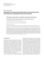
These are the analysis equations that can be implemented
with a filterbank consisting of low- and high-pass filters fol-
lowed with downsamplers. This is demonstrated in Figure 1.
Each single scaling function of the multiscaling function has
ascalarcoefficient associated with it. Hence, C is a column
vector of dimension R. In order to start the filterbank, ini-
tial estimates of the multiscaling function coefficients at the
finest (highest) scale have to be obtained from the samples
of the signal f (t). The signal samples are, thus, preprocessed
N. G
¨
uney and A. Ert
¨

uz
¨
un 3
C
j
G( n)
H(
n)
2
2
C
j 1
D
j 1
Figure 1: The analysis filterbank for orthogonal multiwavelet trans-
form.
(prefiltered) to produce reasonable values for the coefficients
of the multiscaling function at the finest scale [14]. A num-
ber of preprocessing techniques have been proposed for this
purpose. Repeated row (RR) and approximation (AP) pre-
processings are the two most widely used techniques [15]. In
RR preprocessing, the rows of the input vector to the filter-
bank are obtained by scaling the first row consisting of the
signal samples. This preprocessing increases the total num-
ber of samples leading to an oversampling of the original sig-
nal. AP preprocessing, which is based on the approximation
properties of continuous-time wavelets, on the other hand,
yields a critically sampled representation.
2.2. Redundant (undecimated) multiwavelet transform
The procedure for calculating the redundant multiwavelet

transform is based on the work of Mallat in [16] for scalar
wavelets. If R
= 2 and RR (AP) preprocessing is employed on
a 1D signal with length N, the preprocessed signal is 2
× N
(2
×N/2). H(k)are2×2matricesandC
j
(k)are2×1vectors,
H(k)
=

h
1
(k) h
2
(k)
h
3
(k) h
4
(k)

, C
j
(k) =

c
j,1
(k)

c
j,2
(k)

. (8)
Regarding each element of a matr ix filter coefficient as the
coefficient of a scalar filter, h
1
(−k)andh
3
(−k) filter the first,
and h
2
(−k)andh
4
(−k) filter the second row of multiscaling
function coefficients,
c
j−1,1
(k) = c
j,1
(k) ∗h
1
(−k)+c
j,2
(k) ∗h
2
(−k),
c
j−1,2

(k) = c
j,1
(k) ∗h
3
(−k)+c
j,2
(k) ∗h
4
(−k),
(9)
where
∗denotes convolution. In this form, it is apparent that
both rows of multiwavelet and multiscaling function coeffi-
cients at a coarser scale depend on both rows of multiscaling
function coefficients at a finer scale. We have obtained the re-
dundant multiwavelet tr ansform by avoiding downsampling
and padding each of the scalar filters with zeros for upsam-
pling. This has the same effect as padding each of the ma-
trix filter coefficients with zero matrices of size 2
×2. Conse-
quently, the number of redundant multiwavelet coefficients
at each scale is identical (i.e., 2
× N).
3. MULTIRESOLUTION ANALYSIS OF
THE OBJECT BOUNDARY
When a planar object is to be recognized from its image, the
boundary of the object, which is modeled with a 2D curve,
is analyzed. Consider a situation where reference images of
the objects to be recognized are kept in a database, and a test
image taken from a different view of one of the objects is also

present.Thegoalistofindtowhichobjectthistestimage
belongs. Each point (x(t), y(t)) on the boundary curve in the
reference image has been mapped to a point (
x(t), y(t)) on
the curve in the test image,
x(t) = a
0
+ a
1
x( t)+a
2
y(t),
y(t) = b
0
+ b
1
x( t)+b
2
y(t).
(10)
Formulas (10) are combined as
x = Ax + b, (11)
where
A
=

a
1
a
2

b
1
b
2

, b =

a
0
b
0

. (12)
A in (12) is a nonsingular square matrix representing rota-
tion, scaling, and skewing in the affine transformation, and
vector b represents translation.
3.1. The affine-invariant wavelet function
The wavelet coefficients at scale j of the boundary curve in
the test image are related to those of the boundary curve in
the reference image by an equation similar to (11):
W
j
x = AW
j
x, (13)
where W
j
denotes the wavelet “detail” coefficients at scale j.
More clearly,
W

j
x( t) = a
1
W
j
x( t)+a
2
W
j
y(t),
W
j
y(t) = b
1
W
j
x( t)+b
2
W
j
y(t),
(14)
with W
j
a
0
= W
j
b
0

= 0 due to high-pass filtering. An affine-
invariant function is defined in [4] with two scales as
f
i, j
(t) = W
i
x( t)W
j
y(t) −W
i
y(t)W
j
x( t), i = j. (15)
This is a relative invariant, where different affine transforma-
tions of the boundary produce scaled versions of f
i, j
(t), since
it is given by
det

W
i
x W
j
x

= det

A


W
i
x W
j
x

,

f
i, j
(t) = det(A) f
i, j
(t),
(16)
where det(
·) is the determinant.
An a ffine-invariant function with six wavelet scales is
proposed in [4] by introducing a wavelet-based conic equa-
tion using three wavelet scales. The shape descr iptor is the
invariant of two wavelet-based conics with parametrized co-
efficients, where the conics are defined for the scales
{a, b, c}
and {d, e, f }.Different wavelet-based conics are represented
with the two sets of scales. When the coefficients of the con-
ics are solved for, the function η
a,b,c,d,e, f
(t) calculated from
4 EURASIP Journal on Advances in Signal Processing
wavelet scales {a, b, c, d, e, f } is obtained [4]:
η

a,b,c,d,e, f
(t)
=








12W
a
xW
a
yW
2
a
y
12W
b
xW
b
yW
2
b
y
12W
c
xW

c
yW
2
c
y
















W
2
d
x 2W
d
xW
d
y 1
W

2
e
x 2W
e
xW
e
y 1
W
2
f
x 2W
f
xW
f
y 1








+









W
2
a
x 2W
a
xW
a
y 1
W
2
b
x 2W
b
xW
b
y 1
W
2
c
x 2W
c
xW
c
y 1

















12W
d
xW
d
yW
2
d
y
12W
e
xW
e
yW
2
e
y
12W
f

xW
f
yW
2
f
y








−
2








W
2
a
x 1 W
2
a

y
W
2
b
x 1 W
2
b
y
W
2
c
x 1 W
2
c
y

















W
2
d
x 1 W
2
d
y
W
2
e
x 1 W
2
e
y
W
2
f
x 1 W
2
f
y









.
(17)
In (17),
|·|is the determinant, and the dependence of x and
y on the parameter t has been omitted due to limitations of
space. The function is a relative invariant, since it is proven in
[4] to be a sum of products of the relative invariant functions
f
i, j
(t)with{i, j}∈{a, b, c, d, e, f }. An absolute invariant is
obtained in [4] by dividing the relative invariant η(t)with
another one composed of a different set of wavelet scales.
Then, the total number of scales used ranges from 7 to 12
depending on how much overlap between the chosen scales
of the two functions is allowed.
3.2. The affine-invariant multiwavelet function
With MW
j
x
i
(t) denoting the multiwavelet coefficients (de-
tail signal) of the x-coordinate function x(t) of the prepro-
cessed boundary at the ith row and scale j, and taking the
multiwavelet transform of (11), it is observed that multi-
wavelet coefficients at identical rows, which correspond to
the same wavelet ψ
i
(t), are related by an equation similar to
the scalar wavelet case for the jth scale:
⎡

⎣
MW
j
x
i
(t)
MW
j
y
i
(t)
⎤
⎦
=

a
1
b
1
a
2
b
2

⎡
⎣
MW
j
x
i

(t)
MW
j
y
i
(t)
⎤
⎦
, (18)
where i
∈{1,2, , R}. Thus, the affine-invariant function
in (17) can be constructed from the multiwavelet coefficients
by using six sets of coefficients of the form MW
j
x
i
(t), where
at each scale, there are R sets of coefficients.
3.3. The affine-invariant (multi)scaling function
The (multi)scaling function coefficients of the boundary
curve depend on the position of the object in the image, since
the effect of translation b in (12) is not eliminated with low-
pass filtering. This dependence is, however, easily removed
by selecting the centroid of the object as the center of the co-
ordinate system when constructing the affine-invariant func-
tion. Then, the scaling and multiscaling function coefficients
satisfy the same equations that the wavelet and multiwavelet
coefficients do. Although the affine-invariant function η(t)
is constructed in a similar fashion from the (multi)wavelet
and (multi)scaling function coefficients, there is a major

difference between the invariants obtained. Whereas the
(multi)wavelet coefficients at different scales correspond to
orthogonal vector spaces W
j
, the subspaces generated by the
(multi)scaling functions are nonorthogonal. Therefore, the
(multi)scaling function coefficients at different scales are re-
lated.
3.4. The choice of scales
In [4], where the affine-invariant function η(t)isproposed,
and constructed from wavelet coefficients, the first finest
scales have been avoided because they are sensitive to noise.
The effects of quantization are revealed in the finest scale of
wavelet coefficients. The authors in [17], which advocates the
use of scaling function coefficients instead of wavelet coeffi-
cients when constructing invariants, have observed that the
amplitudes of the first few wavelet scales are small and highly
sensitive to noise. As the scale gets coarser, the details of ob-
ject boundaries have been removed from the (multi)scaling
function coefficients by low-pass filtering. Thus, the more
distinguishing features of objects are concentrated in the first
finer-scale (multi)scaling function coefficients.
An object, which is known to belong to a specific
database, is identified via the maximum normalized corre-
lation value between its invariant function and the invari-
ant funct ions of the objects in the database. Thus, six scales
are enoug h to form the invariants, since they are matched by
normalized correlation taking on values in the range [0, 1].
The boundaries of objects are resampled to have a length
of 2

7
and the redundant (multi)wavelet transform is taken
for seven scales. For the multiwavelet transform, the RR pre-
processing is employed with which better recognition per-
formance is observed compared to AP preprocessing. This is
a consequence of the fact that oversampled data representa-
tions are useful for feature extraction [15]. With RR prepro-
cessing, the multiwavelet transform yields seven scales of co-
efficients for the object boundary like in the scalar case. The
chosen scales for the experiments in the next section are as
follows:
(i) wavelet: the finest scale is avoided and the coarsest six
scales are chosen;
(ii) multiwavelet: both rows of the coarsest three scales are
used with R
= 2;
(iii) scaling function: the finest six scales are employed;
(iv) multiscaling function: the finest three scales with both
rows of coefficients are u sed to construct the affine-
invariant function with R
= 2.
4. EXPERIMENTAL RESULTS AND DISCUSSION
In this section, the recognition performance of the affine-
invariant function η(t) constructed with either (multi)wavel-
et or (multi)scaling function coefficients is investigated. Ex-
periments using real airplane images, which are obtained
from [4], are carried out with experimental setups similar to
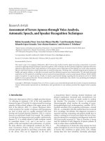
the ones in [4, 6]. The database shown in Figure 2 consists of
20 airplane images in their top view. It contains objects with
very small differences, like models (g) and (t) or (r) and (s).

N. G
¨
uney and A. Ert
¨
uz
¨
un 5
(a) (b) (c) (d) (e) (f) (g) (h) (i) (j) (k) (l)
(m) (n) (o) (p) (q) (r) (s) (t)
Figure 2: The database of airplane object images in their top view.
Theboundariesoftheobjectsareaffine transformed with
the transformation matrix
T
=
⎡
⎣
cos(θ) −sin(θ)
sin(θ)cos(θ)
⎤
⎦
⎡
⎣
2 b
0
1
2
⎤
⎦
, (19)
where θ

∈{0
◦
,36
◦
, , 324
◦
} and b ∈{−2, −3/2, −1, ,
3/2, 2, 5/2
} to realize the unknown object boundar ies. This
makes a total of 100 views for each reference object in the
database. Initially, there exists perfect point correspondence
between the boundary cur ves related by an affine transfor-
mation. For this ideal case of perfect point correspondence,
the normalized correlation is exactly one. Before calculating
the invariant function of the unknown object, u niformly dis-
tributed noise at an SNR of 20 dB is added to the boundary
curve as in [4, 6]. SNR is defined as the ratio of the average
squared distance of the boundary points from the centroid of
the curve to the variance of the uniformly distributed noise.
Uniform distribution takes on values from a finite range de-
termined by its mean and variance. Adding uniformly dis-
tributed noise is realistic in the sense that any boundary
tracking algorithm will find points closely spaced as belong-
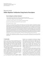
ing to the boundary. When the affine-transformed boundary
of object (i) is disturbed with uniformly distributed white
noise such that SNR
= 20 dB, it appears as in Figure 3.The
noise shifts the samples of the boundary in random direc-
tions. This results in a loss of point correspondence between
the affine-transformed and reference curves, which lowers

the correlation between their invariants.
Point correspondence between the two curves can be
restored, for instance, by finding uniform starting points
for the boundary curves of objects through registering the
shapes based on an analysis of the discrete Fourier se-
ries phase differences [18], and subsequently employing an
affine-invariant parametrization.
The experiments have been performed with four wavel-
ets, two combined sets of wavelets and six multiwavelets:
(1) MZ: the wavelet in [7], w hich is used in [4];
(2) d4: Daubechies 4-coefficient orthogonal wavelet [19];
(3) la8: Daubechies 8-coefficient least asymmetric orthog-
onal wavelet [19];
(4) bi9: 9/7-coefficient symmetric biorthogonal wavelet
[19];
(5) MZ-d4 combination;
0
50
100
150
200
250
300
350
400
5000
500
(a)
0
50

100
150
200
250
300
350
400
5000
500
(b)
Figure 3: The noisy boundary of object (i) at SNR = 20 dB con-
nected with (a) points and (b) lines.
(6) la8-bi9 combination;
(7) GHM: Geronimo-Hardin-Massopust orthogonal sym-
metric multiwavelet [20];
(8) CL: Chui-Lian orthogonal symmetric multiwavelet
[21];
(9) SA4: orthogonal symmetric multiwavelet constructed
by Shen et al. [22];
(10) bih52s: biorthogonal symmet ric multiwavelet [23];
(11) bighm2: bior thogonal multiwavelet obtained from
GHM by factoring out one approximation order [24];
(12) cardbal4: orthogonal cardinal 4-balanced multiwavelet
constructed by Selesnick [25].
For the MZ-d4 and la8-bi9 combinations, the wavelet-coef-
ficient based-invariant is calculated from the coarsest three
scales and when the scaling function coefficients are avail-
able, the finest three scales are made use of. Coefficients of
two wavelets are combined in one invariant in an effort to
make the number of single wavelets applied equal to those

of multiwavelets: the multiwavelets above have R
= 2. The
equations that multiwavelets have to satisfy make it difficult
to construct multiwavelets with R>2.
The boundaries of the objects in the database are affine
transformed using (19), and different realizations of noise
are added to each transformed curve such that SNR
= 20 dB.
The affine-invariant function η(t) calculated from the trans-
formed curve, which is noisy, is correlated with the invariants
of the objects in Figure 2 via

N−1
t=0
η(t)η
i
(t)


N−1
t=0
η
2
(t)

N−1
t=0
η
2
i

(t)
, (20)
6 EURASIP Journal on Advances in Signal Processing
Table 1: Number of correctly matched poses of objects at 20 dB with (multi)wavelet coefficients.
Number of correct matches
Plane MZ d4 la8 bi9 MZ-d4 la8-bi9 GHM CL SA4 bih52s bighm2 cardbal4
(a) 100 87 74 90 100 99 100 100 97 100 100 91
(b)
100 64 71 60 99 78 99 99 100 91 93 99
(c)
100 69 67 62 96 84 98 100 95 95 95 79
(d)
88 72 45 57 94 83 97 98 96 96 87 48
(e)
100 84 84 63 100 95 100 100 100 100 100 100
(f)
94 74 78 62 100 89 100 100 95 98 96 90
(g)
87 42 47 32 99 93 93 95 93 89 82 79
(h)
99 89 73 61 100 100 99 99 98 93 94 95
(i)
97 73 75 72 97 74 88 98 97 93 95 79
(j)
95 68 62 45 100 94 97 93 92 94 95 88
(k)
93 65 61 67 98 85 94 96 93 93 90 75
(l)
84 87 65 44 97 71 99 96 96 96 90 84
(m)

93 57 55 39 98 88 96 95 95 95 90 91
(n)
94 67 66 62 99 84 90 99 100 93 96 70
(o)
97 75 57 48 98 95 99 99 100 99 99 94
(p)
84 55 52 34 98 81 89 94 92 92 81 74
(q)
82 57 69 49 100 76 100 100 99 98 88 80
(r)
100 76 76 63 100 85 97 99 100 100 100 96
(s)
98 69 56 43 99 84 100 99 99 100 97 84
(t)
73 48 16 14 100 74 94 89 99 81 82 47
Average 92.9 68.9 62.5 53.4 98.6 85.6 96.5 97.4 96.8 94.8 92.5 82.15
where i ∈{1, ,20}, η(t)andη
i
(t)oflength2
7
are the in-
variants of the unknown and reference objects, respectively.
The maximum of the correlations identifies the unknown
object.
The recognition performance of the affine-invariant
function construc ted from (multi)wavelet coefficients is dis-
played in Ta ble 1 as the number of correct matches for each
object. In the last row, the average (multi)wavelet perfor-
mance is shown. Although the highest average recognition
rate is achieved by MZ-d4 combination, the multiwavelets

have generally outperformed the scalar wavelets. The func-
tion based on a combination of la8 and bi9 coefficients is a
major improvement over the la8 and bi9 invariants. In addi-
tion, the recognition rates of the (multi)wavelets are seen to
be correlated with the objects, where, for instance, plane (t)
generally has the lowest r a tes among all of the objects. These
observations are related to the approximation properties of
(multi)wavelets.
The subspaces V
j
spanned by translates of (multi)scaling
functions are required to reproduce polynomials up to a cer-
tain degree K
−1[26]. Therefore, as W
j
is orthogonal to V
j
,
the first K moments of the (multi)wavelet vanish,

t
k
Ψ(t)dt = 0, k = 0, , K − 1. (21)
Such a (multi)wavelet has approximation order K. When
R
= 1, the span of φ(t) contains all polynomials of degree
<K. However, when R>1, the span of each indiv idual scal-
ing function φ
i
(t), i ∈{1, , R}, does not have to contain

all such p olynomials [26]. For R
= 1, the degree of polyno-
mials that can be exactly represented by a sum of weighted
and shifted scaling functions is shown to be tied to the num-
ber of zero moments of wavelet filters as well [14]: all mo-
ments of the wavelet (high-pass) filters are zero, μ(k)
= 0for
k
= 0, 1, , K − 1, where
μ(k)
=

n
n
k
g(n). (22)
(Multi)wavelets in this work have approximation orders of 1,
2, or 4:
K
= 1:MZ,SA4,bighm2;
K
= 2: d4, GHM, CL, bih52s;
K
= 4: la8, bi9, cardbal4.
A higher approximation order necessitates an increase in the
length of filter coefficients for wavelets as exemplified by d4
and la8 wavelets.
Theoretically, smoother objects can be represented by
polynomials of lower degree. The (multi)scaling function
coefficients of such objects are sufficient for an accurate

representation and the (multi)wavelet coefficients, which
show the details, have small amplitudes. Hence, the affine-
invariant function η(t) using (multi)wavelet coefficients of
the (multi)wavelets with higher K fails to recognize smoother
objects at a corresponding higher rate. MZ wavelet with the
lowest K is the most successful wavelet in terms of recogni-
tion performance. d4 with K
= 2 comes next and the two
other wavelets, la8 and bi9 having K
= 4, are especially un-
successful with the smoothest object, plane (t). Combining
N. G
¨
uney and A. Ert
¨
uz
¨
un 7
(a) (b) (c) (d)
(e) (f) (g) (h)
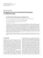
Figure 4: The database of smooth object images.
(a) (b) (c) (d)
(e) (f) (g) (h)
Figure 5: The database of device images.
their wavelet coefficients at the coarser scales so that the finest
scales with small amplitudes are avoided helps to improve
their joint performance when using the wavelet-coefficient
based invariant function. The multiwavelets have generally
high recognition r ates, since their increased dimensionality
makes it possible to disregard the noisy finest scales in the

beginning. The lower number of correct matches for card-
bal4 with K
= 4 justifies the claim about the approximation
properties of (multi)wavelets.
Two image databases have been formed to separate
smooth objects from those that contain more details. They
are shown in Figures 4 and 5,respectively.Thesameexperi-
ment is repeated and the average recognition performance of
(multi)wavelets is given in Ta ble 2. As expected, the average
number of correct matches for wavelets with high K (i.e., la8
and bi9) is very low for smooth objects. The objects in the
device images database have been correctly matched a larger
number of times, since their details have been captured by
the (multi)wavelet coefficients.
Employment of (multi)scaling coefficients when con-
structing the affine-invariant η(t)affects its performance so
muchthatwaveletswithhighK should be preferred over
the multiwavelets. The average recognition rates for the three
databases are given in Table 3. For smooth objects, combin-
ing the scaling function coefficients of two wavelets deteri-
orates the performance of the invariant while this observa-
tion does not hold for the device objects. Among the multi-
wavelets, cardbal4 has exceptionally good recognition perfor-
mance. The average number of correct matches with GHM is
high as well.
As opposed to (multi)wavelet coefficients, which are co-
efficients of basis functions spanning orthogonal spaces,
(multi)scaling function coefficients are obtained from nested
subspaces V
j

which are related. Therefore, when the coeffi-
cients of two different scaling functions are combined, as in
each of the MZ-d4, la8-bi9, or multiwavelet cases, it is es-
sential that the scaling function filters and the approxima-
tion properties of the individual scaling functions a re simi-
lar. Specifically, a constant signal should remain constant af-
ter filtering . Filtering a constant signal c
= 1 with the low-
pass filters of the wavelets and multiwavelets used here pro-
duces the signals c

and [
c
,1
c
,2
]
T
,respectively,whereT is
the transpose:
(i) c

= 1: MZ;
(ii) c

=
√
2: d4, la8, bi9;
(iii) c
,1

=
√
2c
,2
= 1: GHM;
(iv) c
,1
=
√
2c
,2
= 0: SA4, CL, bih52s, bighm2;
(v) c
,1
=
√
2c
,2
=
√
2: cardbal4.
Hence, for some of the multiwavelets, the multiscaling func-
tion coefficients of the boundaries of smoother objects at
different rows should not be jointly used in calculating the
affine-invariant function η(t) which requires them to be
multiplied as in (17). The result is especially catastrophic for
the SA4, CL, bih52s, and bighm2 multiwavelets. The aver-
agenumberofcorrectmatchesinTab le 3 is in compliance
with this observation and cardbal4 rightfully achieves high
recognition rates with an accompanying good performance

for GHM.
The performance of the affine-invariant η(t)isafunction
of the amount of noise on the boundary curve of the object
as well. Thus, a final experiment is made, where the realiza-
tions of noise are produced in such a way that SNR is varied
between 20 dB and 50 dB. The results are shown in Figure 6.
The averages of the correlations (20) between the invariants
obtained from the reference and noisy-affine transformed
curves for the objec ts in Figure 2 are displayed. It is observed
that the invariants based on either the scaling function or the
multiwavelet and the combined sets of wavelet coefficients
are less sensitive to the amount of noise.
5. CONCLUSION
In this work, recognition of planar objects from their test
images which have been obtained from different directions
than their standard view in a database has been consid-
ered. The test images and the reference ones in the database
are related by an affine transformation. Thus, affine in-
variants are required for recognition. Previously, an affine-
invariant function calculated from the wavelet coefficients
of the object boundary has been proposed in [4]. However,
8 EURASIP Journal on Advances in Signal Processing
Table 2: The average number of correct matches at 20 dB with (multi)wavelet coefficients.
Object MZ d4 la8 bi9 MZ-d4 la8-bi9 GHM SA4 CL bih52s bighm2 cardbal4
Smooth 94.3 46.4 37.4 33.5 99.1 92.5 94.9 81.5 93.4 80.8 89.4 72.9
Device
100.0 90.4 84.5 72.0 91.6 79.3 96.4 90.8 95.8 91.4 96.1 96.0
Table 3: The average number of correct matches at 20 dB with (multi)scaling function coefficients.
Object MZ d4 la8 bi9 MZ-d4 la8-bi9 GHM SA4 CL bih52s bighm2 cardbal4
Plane 97.2 96.9 94.3 95.4 78.9 78.0 65.9 29.6 36.9 13.4 14.5 90.0

Smooth
93.1 99.5 99.5 89.6 80.3 80.5 80.4 38.0 41.1 26.8 21.6 93.6
Device
98.5 100.0 98.4 66.5 93.6 93.3 95.0 60.8 63.4 54.9 39.0 97.1
0
0.2
0.4
0.6
0.8
1
Correlation (20)
123456789101112
Type of (multi)wavelet
SNR
= 20 dB
SNR
= 30 dB
SNR
= 40 dB
SNR
= 50 dB
(a)
0
0.2
0.4
0.6
0.8
1
Correlation (20)
123456789101112

Type of (multi)wavelet
SNR
= 20 dB
SNR
= 30 dB
SNR
= 40 dB
SNR
= 50 dB
(b)
Figure 6: The average correlation values (20) for the plane objects
with (a) multiwavelet coefficients and (b) multiscaling function co-
efficients; x-axis corresponds to the (multi)wavelets used in this sec-
tion.
the performance of the function has been tested for only one
view of the object with one type of wavelet. Here, we have cal-
culated the invariant from (multi)wavelet and (multi)scaling
function coefficients of the boundary. An extensive set of
simulations are made, which indicate the following:
(i) multiwavelets have a superior performance compared
to scalar wavelets when the detail coefficients are avail-
able. For smooth objects, the result is more pro-
nounced;
(ii) the scaling function coefficients of two different scal-
ing functions should not be used jointly in one invari-
ant function due to the fact that the scaling func tion
coefficients at different scales are expected to be corre-
lated;
(iii) the scaling function coefficients are more stable com-
pared to wavelet coefficients in the presence of noise.

The observations above are shown to be closely related to
multiresolution analysis and the approximation properties of
(multi)wavelets.
ACKNOWLEDGMENT
The authors would like to thank Vasily Strela for generously
providing his multiwavelet software package (MWMP),
where the coefficients for most of the (multi)wavelets used
in this paper can be found.
REFERENCES
[1] I. Weiss, “Geometric invariants and object recognition,” Inter-
national Journal of Computer Vision, vol. 10, no. 3, pp. 207–
231, 1993.
[2] K. Arbter, W. E. Snyder, H. Burkhardt, and G. Hirzinger, “Ap-
plication of affine-invariant Fourier descriptors to recognition
of 3-D objects,” IEEE Transactions on Pattern Analysis and Ma-
chine Intelligence, vol. 12, no. 7, pp. 640–647, 1990.
[3] R. Alferez and Y F. Wang, “Geometric and illumination in-
variants for object recognition,” IEEE Transactions on Pattern
Analysis and Machine Intelligence, vol. 21, no. 6, pp. 505–536,
1999.
[4] M. I. Khalil and M. M. Bayoumi, “A dyadic wavelet affine in-
variant function for 2D shape recognition,” IEEE Transactions
on Pattern Analysis and Machine Intelligence, vol. 23, no. 10,
pp. 1152–1164, 2001.
N. G
¨
uney and A. Ert
¨
uz
¨

un 9
[5] Q.M.TiengandW.W.Boles,“Wavelet-basedaffine invari-
ant representation: a tool for recognizing planar objects in 3D
space,” IEEE Transactions on Pattern Analysis and Machine In-
telligence, vol. 19, no. 8, pp. 846–857, 1997.
[6] E. Bala and A. E. Cetin, “Computationally efficient wavelet
affine invariant functions for shape recognition,” IEEE Trans-
actions on Pattern Analysis and Machine Intelligence, vol. 26,
no. 8, pp. 1095–1099, 2004.
[7] S. Mallat and S. Zhong, “Characterization of signals from mul-
tiscale edges,” IEEE Transactions on Pattern Analysis and Ma-
chine Intelligence, vol. 14, no. 2, pp. 710–732, 1992.
[8] M. B. Martin and A. E. Bell, “New image compression tech-
niques using multiwavelets and multiwavelet packets,” IEEE
Transactions on Image Processing, vol. 10, no. 4, pp. 500–510,
2001.
[9] T. D. Bui and G. Chen, “Translation-invariant denoising using
multiwavelets,” IEEE Transactions on Signal Processing, vol. 46,
no. 12, pp. 3414–3420, 1998.
[10] E. Bala and A. Ert
¨
uz
¨
un, “A multivariate thresholding tech-
nique for image denoising using multiwavelets,” EURASIP
Journal on Applied Signal Processing, vol. 2005, no. 8, pp. 1205–
1211, 2005.
[11] F. P. Nava and A. F. Martel, “Planar shape representation based
on multiwavelets,” in Proceedings of 10th European Signal Pro-
cessing Conference (EUSIPCO ’00), Tampere, Finland, Septem-

ber 2000.
[12] T. N. T. Goodman and S. L. Lee, “Wavelets of multiplicity r,”
Transactions of the American Mathematical Society, vol. 342,
no. 1, pp. 307–324, 1994.
[13] V.Strela,P.N.Heller,G.Strang,P.Topiwala,andC.Heil,“The
application of multiwavelet filterbanks to image processing,”
IEEE Transactions on Image Processing, vol. 8, no. 4, pp. 548–
563, 1999.
[14] C. S. Burrus, R. A. Gopinath, and H. Guo, Introduction to
Wavelets and Wavelet Transforms, Prentice-Hall, Upper Saddle
River, NJ, USA, 1998.
[15] V. Strela, Multiwavelets: theory and applications,Ph.D.the-
sis, Massachusetts Institute of Technology, Cambridge, Mass,
USA, 1996.
[16] S. Mallat, “Zero-crossings of a wavelet transform,” IEEE Trans-
actions on Information Theory, vol. 37, no. 4, pp. 1019–1033,
1991.
[17] I. El Rube, M. Ahmed, and M. Kamel, “Wavelet approx-
imation-based affine invariant s hape representation func-
tions,” IEEE Transactions on Pattern Analysis and Machine In-
telligence, vol. 28, no. 2, pp. 323–327, 2006.
[18] M. J. Paulik and Y. D. Wang, “Three-dimensional object recog-
nition using vector wavelets,” in Proceedings of the IEEE Inter-
national Conference on Image Processing, vol. 3, pp. 586–590,
Chicago, Ill, USA, October 1998.
[19] I. Daubechies, Ten Lectures on Wavelets, SIAM, Philadelphia,
Pa, USA, 1992.
[20] G. S. Geronimo, D. P. Hardin, and P. R. Massopust, “Fractal
functions and wavelet expansions based on several functions,”
Journal of Approximation Theory, vol. 78, no. 3, pp. 373–401,

1994.
[21] C. K. Chui and J. A . Lian, “A study of orthonormal multi-
wavelets,” CAT Report 351, Texas A&M University, Canyon,
Tex, USA, 1995.
[22]L X.Shen,H.H.Tan,andJ.Y.Tham,“Symmetric-
antisymmetric or thonormal multiwavelets and related scalar
wavelets,” Applied and Computational Harmonic Analysis,
vol. 8, no. 3, pp. 258–279, 2000.
[23] R. Turcajova and V. Strela, “Smooth hermite spline multi-
wavelets,” in preparation.
[24] V. Strela, “A note on construction of biorthogonal multi-
scaling functions,” in Contemporary Mathematics, A. Aldroubi
and E. B. Lin, Eds., vol. 216, pp. 149–157, American Mathe-
matical Society, Providence, RI, USA, 1998.
[25] I. Selesnick, “Cardinal multiwavelets and the sampling theo-
rem,” in Proceedings of the IEEE International Conference on
Acoustics, Speech, and Signal Processing (ICASSP ’99), vol. 3,
pp. 1209–1212, Phoenix, Ariz, USA, March 1999.
[26] K. Berkner and P. R. Massopust, “Translation invariant mul-
tiwavelet transforms,” Tech. Rep. CML TR 98-06, Computa-
tional Mathematics Laboratory, Rice University, Houston, Tex,
USA, 1998.
Nazlı G
¨
uney received the B.S. (with high
honors) and M.S. degrees in electr ical and
electronics engineering from Bo
¯
gazic¸i Uni-
versity, Istanbul, Turkey, in 2001 and 2003,

respectively, and she is currently working
toward the Ph.D. degree in electrical and
electronics engineering from Bo
¯
gazic¸i Uni-
versity. Since 2001, she has been a Research
and Teaching Assistant with Bo
¯
gazic¸i Uni-
versity. She worked on planar object recog-
nition for her M.S. thesis. Her current research interests include
various aspects of UWB communications with special emphasis on
design and analysis of robust systems for non-Gaussian channels.
Ays¸ın Ert
¨
uz
¨
un was born in 1959 in Salihli,
Turkey. She received the B.S. degree (with
honors) from Bo
¯
gazic¸i University, Istanbul,
Turkey, the M.Eng. degree from McMaster
University, Hamilton, Ontario, Canada, and
the Ph.D. degree from Bo
¯
gazic¸i University,
Istanbul, Turkey, all in electrical engineer-
ing, in 1981, in 1984, and in 1989, respec-
tively. Since 1988, she has been with the De-

partment of Electrical and Electronics En-
gineering at Bo
¯
gazic¸i University where she is currently a Profes-
sor. Her current research interests are in the areas of independent
component analysis and its applications, blind signal processing,
Bayesian methods, application of wavelets and adaptive systems
to communication systems, image processing, and texture analy-
sis. She has authored and coauthored nearly 70 scientific papers in
journals and conference proceedings. She is a Member of IEEE Sig-
nal Processing and Communication Societies, International Asso-
ciation of Pattern Recognition (IAPR), The Institute of Electronics,
Information and Communication Eng ineers (IEICE), and Turkish
Pattern Recognition and Image Processing Society (TOTIAD).