Báo cáo hóa học: " Research Article Separation and Localisation of P300 Sources and Their Subcomponents Using Constrained Blind Source Separation" pot

Hindawi Publishing Corporation
EURASIP Journal on Advances in Signal Processing
Volume 2007, Article ID 82912, 10 pages
doi:10.1155/2007/82912
Research Article
Separation and Localisation of P300 Sources and Their
Subcomponents Using Constrained Blind Source Separation
Loukianos Spyrou,
1
Min Jing,
1
Saeid Sanei,
1
and Alex Sumich
2
1
The Centre of Digital Signal Processing, School of Engineering, Cardiff University, Queen’s Buildings, P.O. Box 925,
Newport Road, Cardiff CF24 3AA, Wales, UK
2
The Brain Image Analysis Unit, Institute of Psychiatry, King’s College Hospital, London SE5 8AF, UK
Received 1 October 2005; Revised 31 May 2006; Accepted 11 June 2006
Recommended by Frank Ehlers
Separation and localisation of P300 sources and their constituent subcomponents for both visual and audio stimulations is in-
vestigated in this paper. An effective constrained blind source separation (CBSS) algorithm is developed for this purpose. The
algorithm is an extension of the Infomax BSS system for which a measure of distance between a carefully measured P300 and the
estimated sources is used as a constraint. During separation, the proposed CBSS method attempts to extract the corresponding
P300 signals. The locations of the corresponding sources are then estimated with some indeterminancy in the results. It can be
seen that the locations of the sources change for a schizophrenic patient. The experimental results verify the statistical significance
of the method and its potential application in the diagnosis and monitoring of schizophrenia.
Copyright © 2007 Loukianos Spyrou et al. This is an open access article distributed under the Creative Commons Attribution
License, which permits unrestricted use, distribution, and reproduction in any medium, provided the original work is properly

cited.
1. INTRODUCTION
Event-related potentials (ERPs) are those electroencephalo-
grams (EEGs) which directly measure the electrical response
of the cortex to sensory, affective, and/or cognitive events.
The fine-grained temporal resolution offered by ERPs allows
accurate study of the time course of information process-
ing unavailable to other neuroimaging techniques. However,
spatial resolution has been traditionally limited. In addition,
overlapping components of the ERP which represent sp ecific
stages of information processing are difficult to distinguish
[1, 2]. An example is the composite P300 wave, a positive
ERP component which occurs with a latency of about 300
milliseconds after novel stimuli, or task relevant stimuli, re-
quiring an effortful response on the part of the individual un-
der test [1–5]. The P300 wave represents cognitive functions
involved in orientation of attention, contextual updating , re-
sponse modulation, and response resolution [1, 3], and con-
sists of multiple overlapping subcomponents, two of which
are identified as P3a and P3b [2, 5]. P3a reflects an automatic
orientation of attention to novel or salient stimuli indepen-
dent of task relevance [5, 6]. Prefrontal, frontal, and anterior
temporal brain regions play a major role in generating P3a
giving it a frontocentral distribution [1, 5]. In contrast, P3b
has a greater centroparietal distribution due to its reliance on
posterior temporal, parietal, and poster ior cingulate mecha-
nisms [1, 2]. P3a is also characterised by a shorter latency and
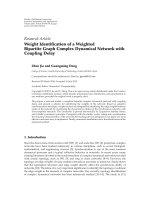
more rapid habituation than P3b [2, 5]. Figure 1 illustra tes
some typical P3a and P3b waveforms from temporal-basal
and temporo-superior dipoles [7].

Abnormalities in P300 are found in several of psychi-
atric and neurological conditions [4], however, differences
may exist in particular in the specific subcomponents [2].
Moreover, changes to certain P300 subcomponents m ay dis-
tinguish between relatives discordant for psychiatric illness,
and between subdiagnosis of illness [8, 9]. That is, although
reduced amplitude of the auditory P300 is reported in almost
all studies of schizophrenia, the nature of these reductions
including topography and associated subcomponents varies
with subdiagnosis and sex [8, 10]. Finally, certain subcom-
ponents may be modality specific, whilst others may be in-
dependent of modality [2]. Thus, auditory and visual P300
appear to be differentially affected by illness and respond dif-
ferently to treatment, suggesting differences in underlying
structures and neurotransmitter systems [2]. P300 has sig-
nificant diagnostic and prognostic potential especially w hen
combined with clinical evaluation [2, 4]. However, in order
for this to be fully realised, efficient and reliable methods for
2 EURASIP Journal on Advances in Signal Processing
1
P3b
2
P3b
3
P3a
4
P3a
2
1
43

Figure 1: Some examples for P3b (1 and 2) and P3a (3 and 4) sig-
nals and their corresponding typical locations.
separating P300 sources and its subcomponents must be es-
tablished [4].
Blind source separation (BSS) has been used to identify
the ERP subcomponents [11].TheobjectiveofBSSistosepa-
rate a number of sources (component generators) from their
mixtures (elect rode signals). This is achieved by using infor-
mation only from the sensor signals and, if available, some
information about the statistical properties of the sources.
Successfully performing BSS is a challenging problem in a
variety of real-world applications. Various algorithms have
been developed depending on specific applications [11]. A
family of BSS algorithms stems from the principle of inde-
pendent component analysis (ICA). This method tries to es-
timate the sources by assuming that they a re statistically in-
dependent.
The most common method in detection, highlighting,
and visualisation of P300 components used by clinicians is
the frame averaging method. The problem has been tackled
in more mathematical ways and one of the first approaches
was to estimate brain sources, obtained from an electroen-
cephalogram (EEG) or magnetoencephalogram (MEG), us-
ing a least-squares approach [12, 13]. ICA was used later by
a number of authors [14, 15]. The motivation was to ex-
tract sources of electrical activity which represent different
brain functions (i.e., they are independent). These authors
used the Infomax [16] algorithm which produced satisfac-
tory results in terms of source separation. In this paper, we
develop a constrained algorithm based on Infomax to sepa-

rate P300 sources and their subcomponents. The constraint
term is achieved based on a prior knowledge of some measur-
able properties of the sources such as their latencies. A simi-
lar method has been developed in [17, 18]whichemploysa
constrained ICA algorithm using reference signals. However,
the type of constraint and they way it is constructed are dif-
ferent. Here, we also emphasize on the development an au-
tomatic detection and localisation procedure for the P3a and
P3b subcomponents.
The paper is structured as follows. Section 2 describes the
basic B SS model and principles. Section 3 describes the pro-
posed methods for separation and localisation of the P300
components. Section 4 shows some experimental results
obtained by applying the proposed methods to EEGs
recorded from some normal subjects and schizophrenic pa-
tients as well as some simulated data. Section 5 concludes the
paper.
2. BLIND SOURCE SEPARATION
Regarding EEG, the mixing process is assumed instantaneous
and the model is defined as fol lows: there is a number m of
sensor signals x(t)
= [x
1
(t), x
2
(t), , x
m
(t)]
T
and a number

n of source signals s(t)
= [s
1
(t), s
2
(t), , s
n
(t)]
T
. The mixing
system is described by the matrix H
∈ R
m×n
and the relation
between the sensors and the sources is
x(t)
= Hs(t). (1)
The element h
ij
of the matrix H is the mixing coefficient
from the jth source to the ith electrode. All signals are as-
sumed zero mean or can be made so by subtracting the mean
from them, additive observation noise is assumed insignifi-
cant. The aim of B SS is to estimate the original sources using
information only from the sensors x(t). In most cases a ma-
trix W
= H
−1
is used to estimate the sources indirectly by
y(t)

= s(t) = Wx(t), (2)
where
s(t) denotes the estimate of s(t). In ICA the source sig-
nals are treated as random variables and the statistical prop-
erties of the signals are used to obtain the unmixing matrix. If
each source i
= 1, , n is assumed to have a probability den-
sity function (pdf) q
i
(·), the independence assumption can
be expressed mathematically as follows: the joint pdf q(s)of
the source vector s is equal to the product of the marginal
pdfs:
q(s) = q
1

s
1

···
q
n

s
n

=
n

i=1

q
i

s
i

. (3)
The ICA algorithm usually depends on the assumption made
for the pdfs of the sources q
i
(s
i
). Also, since a closed-form
solution to the ICA equation does not exist or it is gener-
ally very difficult to obtain, a cost function J(W), which pro-
vides a measure of independence, is optimised in an iterative
manner using an optimisation technique such as a form of
steepest descent or Newton’s method. There are two main
problems associated with the ICA method. Firstly, the esti-
mated sources can be a scaled version (potentially with a sign
change) of the original sources and, secondly, there is no way
of knowing the order of the sources. These two problems are
known, respectively, as the scaling and permutation ambi-
guities. The scaling problem may be mitigated by normal-
ising the results with respect to the geometrical dimensions
of the head. The permutation problem, however, has negli-
gible effect in this application context as will be discussed in
Section 4.
3. PROPOSED METHODS
3.1. Constrained BSS

The Infomax algorithm was used as the original cost function
since it has been reported to be effective for the separation
Loukianos Spyrou et al. 3
of EEG signals [14, 15]. The Infomax algorithm attempts
to maximise the information flow between the inputs and
the outputs of an artificial neural network (ANN). In this
case, the inputs are the electrode signals and the outputs are
some nonlinear transformation of the estimated sources. It
is shown that if the nonlinear functions a re selected appro-
priately [16], then the information maximisation will corre-
spond to the minimisation of the dependence between the
estimated sources. The Infomax cost function is
J
m
(W) = I(z, x) = H(z) − H

z | x

,(4)
where z
∈ R
n×1
is the output of the neural network (z =
f (y), f (·) is the nonlinear activation function applied ele-
ment wise to y which is the estimated source vector), x is the
input to the neural network, I(z, x) is the information be-
tween the inputs and the outputs of the ANN, H(z) is the
entropy of the output and H(z
| x) is the conditional en-
tropy of the output assuming a known input; note, for con-

venience, the time index is dropped. The natural gradient of
(4)is
∇
W
I(z, x)W
T
W =∇
W
H(z)W
T
W (5)
since H(z
| x) is independent of W. Maximisation based
on the natural gradient is used to achieve good convergence
[19]. The adaptation rule for the unmixing matrix W be-
comes
W
t+1
= W
t
+ μ

I +

1 − 2 f (y)

y
T

W,(6)

where f (y)
=(1 +exp(−y))
−1
with the assumption of super-
Gaussian outputs and μ is the learning rate. The adaptation
for an individual weight can be described by the equation
(using the gradient ascent method)
Δw
ij
=
cof w
ij
det W
+ x
j

1 − 2y
i

,(7)
where cof represents the cofactor and det the determinant.
Thus, each individual weight is adapted in a way that the
rows and columns differ from each other, as prescribed by the
first term of the right-hand side of the equation. When two
rows or columns b ecome similar, the matrix becomes singu-
lar, and then det W will tend to zero forcing the weight ele-
ment to change dramatically. This change will be affected by
cof w
ij
which shows the relative singularity of the remainder

of the matrix, regardless of the row and column this element
belongs to, compared to the whole of the matrix.
ICA in general does not produce unique outputs and we
aim to develop an algorithm that ensures that the desired
P300 source is one of the estimated sources. This can be
achieved by adding a constraint to the original algorithm. La-
grange multipliers incorporate the constraint function into
the original cost function. This changes the problem into an
unconstrained one. The constraint is considered as the Eu-
clidean distance between the estimated sources and a refer-
ence P300 signal. The reference signal is obtained by frame
averaging of the ERP obtained from a number of trials. The
constrained problem can be written as
max J
m
(W)subjecttoJ
C
(W) = 0, (8)
J
m
and J
C
are the Infomax and the constrained cost functions,
respectively. The cost function of the CBSS J algorithm is
J(W, Λ)
= J
m
(W) − ΛJ
C
(W), (9)

where Λ is the matrix of the Lagrange multipliers. The con-
straint function specialised for each column of W is defined
as
J
C

w
i

=
P

t=1

y
i
(t) −r(t)

2
for i = 1, , m, (10)
where r(t) is the reference signal and y
i
(t) is the ith output
at time t. The unknown parameters in the problem are now
two: the matrix W and the matrix Λ.ThematrixW is found
adaptively via the following relation [20]:
W
t+1
= W
t

+ μ

∇
W
t
J

W
t
, Λ

W
T
t
W
t
= W
t
+ μ

I +

1 −

1+exp

W
t
x


−1

W
t
x

T
− 2Λ

x

W
t
x − P

T

W
T
t

W
t
,
(11)
Λ
= ρ diag

(Wx − P)(Wx − P)
T


, (12)
where μ is the learning rate of the adaptation of the unmixing
matrix, ρ is a scale factor for the Lagrange multiplier matrix,
and P is a matrix whose rows contain the reference P300 sig-
nal. If a block algorithm is required, then the data vector x
becomes a matrix and it should be scaled accordingly.
The basic form of the constrained algorithm can be mod-
ified to mitigate some inherent problems with this approach.
Firstly, the present form of the algorithm tries to produce n
outputs that are as close as possible to the P300 reference sig-
nal. Although this effect is alleviated partly by the Infomax
algorithm which tries to produce different outputs, the con-
straint part of the algorithm will try and adjust more those
outputs that are further away (in Euclidean distance terms)
from the reference signal. Hence, it would be a good idea to
try to enforce the constraint in one or a small number of the
outputs. This comes from the fact that usually the P300 sig-
nal consists of a number of subcomponents in different re-
gions of the brain. Secondly, the scaling ambiguity of every
ICA algorithm can be a problem since one output could have
exactly the same shape as the reference signal but it could
be a scaled version of it. The algorithm would change that
output (since it violates the constraint) which could dam-
age its shape. So, a scaling procedure is used in which the
reference signal matches the maximum amplitude of the es-
timated sources. Finally, the problem of finding good initial
conditions for W, Λ, μ,andρ,canbeovercomepartlyby
using a variable which determines the contribution of the
two separate cost functions (i.e., main and constraint) to

the adaptation of W. This way, the algorithm can be made
to work (by avoiding the rapid divergence of the Frobenius
norm of W) in a variety of situations. This way, the stabil-
ity of the algorithm is ensured because the learning is kept
bounded especially when J
c
(w
i
)  0.Italsofunctionsasa
safety point to make sure that the algor ithm converges to a
4 EURASIP Journal on Advances in Signal Processing
solution, which produces outputs close to the reference sig-
nals. The convergence of the algorithm is stable to the opti-
mum point since both parts of the CBSS function have a neg-
ative definite Hessian matrix (easy to prove by checking the
sign and the nonsingularity of the Hessian). The constrained
cost function can take any form that would be suitable for
a specific application. A cost function which maximises the
inner product between the estimated sources and the refer-
ence signals was used but its performance was not as satisfac-
tory as the Euclidean distance function. Following the the-
ory of constrained optimisation, in cases where the separa-
tion needs to be improved over the traditional ICA methods,
a number of new BSS algorithms can be developed. Other
suggested cost functions for the present purpose can be max-
imising the spikiness of the output sources around the time
of interest (300 milliseconds), estimating the pdf of the P300
sources and forcing the pdfs of the output sources to have
a similar form
1

or even applying a spatial constraint using
prior knowledge of the possible P300 positions.
A variation of this algorithm wh ich was used to separate
the P3a and P3b subcomponents was implemented by using
the method of least squares. If the reference signals for P3a
and P3b are known, then we can model the EEG system as
r
= w
opt
X, (13)
where r is the reference signal, X is the data matrix, and w
opt
(row vector 1 × n) is the vector that should produce r.Then,
the constraint cost function will be
J
C

w
i

=


w
i
− w
opt


2

2
, (14)
where w
i
is the ith row vector of the unmixing matrix. This
vector corresponds to the ith output y
i
expected to be the
separated P3a or P3b. The selection of the appropriate y
i
to
enforce the constraint is achieved in terms of which one is
closer in terms of the Euclidean distance to the reference sig-
nal. w
opt
is found using the common least-squares (LS) solu-
tion:
w
T
opt
=

XX
T

−1
Xr
T
. (15)
Also, the gradient of (14)is

∇
w
i
J
C

w
i

= 2

w
i
− w
opt

. (16)
Then, this gradient is incorpora ted within the main Infomax
update equation in a similar manner to ( 11 ). This constraint
is different from those used in [17, 18 ].
3.2. Construction of the reference signals and
detection of P300 subcomponents
P3a and P3b are the two P300 subcomponents that overlap
at the scalp. A constrained BSS algorithm such as that de-
scribed above can be used to extract the P3a and P3b from
1
This can be facilitated as part of the original Infomax algorithm where the
activation function should ideally be derived from the pdfs of the sources.
multichannel EEGs. One important factor in applying CBSS
is the selection of the proper reference signal. The way we

obtain the reference signals is to use prior knowledge of the
latencies of the two subcomponents. P3a peaks on average
at a latency of 260 milliseconds and P3b on average at 300
milliseconds. However, it is possible that both the P3a and
P3b occur with different latencies. The distinctive feature is
then that P3a occurs before the P3b. P3a is hence selected by
space-time averaging all the electrodes and selecting the first
peak that occurs near the time of interest (250 milliseconds–
350 milliseconds) and P3b by selecting the second peak. The
two reference signals are then used in the CBSS algorithm. To
detect which of the CBSS outputs is the P3a and which is the
P3b, we use the correlation function. For two variables x and
y, the correlation coefficient is defined as
cor(x, y)
=
cov(x, y)
σ
x
σ
y
, (17)
where σ
x
denotes the standard deviation and cov(x, y) the
covariance of the two variables. The covariance of the two
variables provides a measure of how strongly correlated these
variables are. Because our purpose is to detect P3a and P3b,
the source which has the maximum correlation coefficient
with the P3a or P3b reference signal is more likely to be P3a
or P3b, which will be selected automatically.

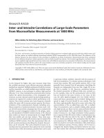
3.3. Localisation
Localisation of electrical sources inside the brain has been in-
vestigated by a number of people [12, 13, 21–23]. Unlike the
work done in [12] which assumes that the electrical sources
are magnetic dipoles, here we assume that they are sources
of isotropic propagation. Hence, the head simply mixes and
attenuates the signals. Therefore based on Figure 2 we have


f
k
− a
j


2
= d
j
for j = 1, 2, 3, (18)
where f
k
is the position of the source k, a
j
are the positions
of the electrodes, and d
j
are the distances between the source
and the jth electrode. The distances d
j
are nonlinearly pro-

portional to the inverse of the correlation between the es-
timated source and the elec trode signals. This is because a
source is attenuated nonlinearly with the distance. Hence, the
correlation of the electrodes with a source is nonlinearly pro-
portional to the distance [24]:
cor

X, s
k

=

X · s
k

= HSs
T
k
, (19)
where X
= HS, H describes the forward model for which the
magnitude of a source attenuates with 1/d
2
j
,ands
k
is the vec-
tor of all sample values of the kth source. It has to be noted
that the sources must be uncorrelated for the method to be
efficient. After computing the correlation the values are nor-

malised and converted to distances by the following:
d
j
=
1
√
cor
. (20)
It has to be noted that this approach does not provide
a valid source reconstruction since it ignores the conduc-
tivity properties of the brain but it can be used to distin-
guish between sources in relatively different locations. Index
Loukianos Spyrou et al. 5
Scalp
a1
a2
a3
d
1
d
2
d
3
f
k
Figure 2: Part of the scalp including the electrode locations, a1, a2,
and a3, and the location of the source k, f
k
, to be identified.
j represents the three electrodes that have maximum corre-

lation coefficients with source k, k
= 1, 2, , n, showing the
source number. In this equation all the variables except f
k
are
known.
Thenextstepistoconverttoamathematicalproblem,
which is required to calculate the coordinates of an unknown
point when both of the coordinates of d points and the
distances of the unknown point from the given points are
known. This problem is clearly equivalent to finding the in-
tersection point(s) of d spheres in R
d
. The points are the so-
lution to the following least-squares problem which can be
obtained from [25]:
min S

f
k

,withf
k
∈ R
d
, (21)
where
S

f

k

=
3

j=1



f
k
− a
j


2
− d
j

2
. (22)
4. EXPERIMENTAL RESULTS
4.1. Simulated data experiment
The CBSS algorithm was firstly applied to simulated data to
test its e fficacy. Two sinusoidal sources and one sinc signal
(simulating the P300 as in Figure 3)weremixed(Figure 4).
The results from the original Infomax algorithm were com-
pared with those of the CBSS algorithm. The same learning
rate (μ
= 0.001) and initial conditions (W

0
= I) were used
in both cases. Figures 5 and 6 show, respectively, the esti-
mated P300 source using the two algorithms. The original
sinc source was used as the reference. The performance was
measured with the mean square error:
error
= 10 log
1
N
N

i=1

s(i) − s(i)

2
, (23)
where N is the number of samples,
s(i) is the obtained source,
and s(i) is the original source and the error is given in dB. The
P300 obtained from normal Infomax had an error of e
=
−
18.9 dB while that of CBSS had an error of e =−19.8dB.
The CBSS algorithm used was that of (11).
012345
Time
1
0

1
Amplitude
012345
Time
1
0
1
Amplitude
012345
Time
0.5
0
0.5
1
Amplitude
Figure 3: A set of synthetic sinusoidal sources with a sinc function
emulating the P300 source.
012345
Time
2
0
2
Amplitude
012345
Time
5
0
5
Amplitude
012345

Time
5
0
5
Amplitude
Figure 4: The mixtures obtained by mixing the sources of Figure 3
using a random mixing matrix.
4.2. Separation and localisation of the P3a and P3b
4.2.1. Experiment data
The EEG data were recorded using a Nihon Kohden model
EEG-F/G amplifier and Neuroscan Acquire 4.0 software.
EEG activity was recorded following the international 10–
20 system from 15 electrodes. The reference electrodes were
linked to the earlobes. The impedance for all the electrodes
was below 5 kΩ, sampling frequency Fs
= 2 kHz, and the
6 EURASIP Journal on Advances in Signal Processing
00.511.522.5
Time (ms)
2
1
0
1
2
3
4
5
6
7
Amplitude

Figure 5: The estimated P300 source using the proposed CBSS.
CBSS achieves a slightly better representation but with a decrease
in mean square error than normal Infomax.
00.511.522.5
Time (ms)
2
1
0
1
2
3
4
5
6
7
8
Amplitude
Figure 6: The estimated P300 sources using Infomax. The simu-
lated P300 is slightly more distorted than that obtained by CBSS
and achieves a higher mean square error.
data were subsequently bandpass filtered (0.1–70 Hz). This
frequency range was chosen to be compatible with [26].
The EEG data were recorded for control and schizo-
phrenic patients. The Diagnostic and Statistical Manual of
Mental Disorders 4th edition (DSM-IV) Axis 1 disorders was
used to confirm diagnosis of schizophrenia. Subjects were re-
quired to sit alert and still with their eyes closed to avoid any
interference. Also, to avoid any muscle artefact, the neck was
firmly supported by the back of the chair. The feet were rested
on a footstep. The stimuli were presented through ear plugs

inserted in the ear. Forty rare tones (1 kHz) were randomly
distributed amongst 160 frequent tones (2 kHz). Their in-
tensity was 65 dB with 10- and 50-milliseconds duration for
0 200 400 600 800 1000
Time (ms)
5
0
5
10
FZ
0 200 400 600 800 1000
Time (ms)
10
0
10
20
CZ
0 200 400 600 800 1000
Time (ms)
5
0
5
10
PZ
Figure 7: Three channel ERP of a schizophrenic patient obtained
by averaging 40 related events.
rare and frequent tones, respectively. The subject was asked
to press a button as soon as they heard a low tone (1 kHz).
The ability to distinguish between low and high tones was
confirmed before the start of the experiment. The task is de-

signed to assess basic memory processes. ERP components
measured in this task included N100, P200, N200, and P3a
and P3b.
4.2.2. Separation of P3a and P3b
Firstly, the ERP is obtained by temporally averaging event-
related data (40 events), each event producing an EEG of size
n
×T,wheren is the number of electrode signals and T is the
number of samples of the event. That averaged ERP is also of
dimensions n
× T. The advantage of averaging event-related
data is not only to enhance the signal, but also to remove
non-event-related noise. Secondly, the reference subcompo-
nent signal is selected according to the method described in
Section 3.2. Thirdly, CBSS is applied to the ERP (n
× T)in
order to separate the P300 and its sub-components. Filter-
ing (at the Delta range) is applied to the separated sources,
based on the knowledge that the main power of the P300
component is in the Delta range [27]. Figure 7 shows the ERP
and Figure 8 shows the estimated P3a and P3b sources for a
schizophrenic patient. Figure 9 shows the ERP and Figure 10
shows the estimated P3a and P3b for a control subject. It can
be seen that the P3a component is earlier in latency than the
P3b.
4.2.3. Localisation of P3a and P3b
To approximately specify the location of a source in the
head, we consider a spherical model of the head and as-
sume isotropic propagation of the sources. Using the method
Loukianos Spyrou et al. 7

0 100 200 300 400 500 600 700 800 900 1000
Time (ms)
5
0
5
P3a
0 100 200 300 400 500 600 700 800 900 1000
Time (ms)
4
2
0
2
4
6
P3b
Figure 8: The separated P3a and P3b from the signals of Figure 7
using the proposed CBSS algorithms.
0 200 400 600 800 1000
Time (ms)
10
0
10
FZ
0 200 400 600 800 1000
Time (ms)
10
0
10
CZ
0 200 400 600 800 1000

Time (ms)
10
0
10
PZ
Figure 9: Three channel ERPs of a control subject obtained by av-
eraging 40 related events.
described in Section 3, there may be some trivial solutions
(i.e., the points which fall outside the head) which are auto-
matically discarded based on geometrical constraints.
The result of the localisation of the P3a and P3b com-
ponents is shown in Figure 11 for five schizophrenic patients
and in Figure 12 for five control subjects. It is evident that
the P3a and P3b for a schizophrenic patient are closely and
irregularly located, whereas for a control subject the P3a and
P3b are located in distinct regions.
0 200 400 600 800 1000
Time (ms)
4
2
0
2
4
6
P3a
0 200 400 600 800 1000
Time (ms)
4
2
0

2
4
6
P3b
Figure 10: The separated P3a and P3b from the signals of Figure 9
using the proposed CBSS algorithm.
Figure 11: Localisation result for schizophrenic patients. The circles
correspond to the P3a and the squares to P3b. The P3a and P3b are
closely and ir regularly located following no specific pattern.
Figure 12: Localisation result for normal subjects. The circles cor-
respondtoP3aandthesquarestoP3b.TheP3aandP3bsourcesare
located in distinct regions in the brain.
8 EURASIP Journal on Advances in Signal Processing
0 100 200 300 400 500 600 700 800 900 1000
Time (ms)
5
0
5
Amplitude
0 100 200 300 400 500 600 700 800 900 1000
Time (ms)
5
0
5
10
Amplitude
0 100 200 300 400 500 600 700 800 900 1000
Time (ms)
2
1

0
1
2
Amplitude
Figure 13: The top figure shows the output obtained by normal
Infomax while the middle figure shows the CBSS output and the
bottom figure shows the reference signal for a schizophrenic patient.
4.2.4. Comparison between CBSS and Infomax
Some obtained P3a using normal unconstrained Infomax
and CBSS is shown here. The results from normal Infomax,
CBSS, and the reference signal are shown in Figures 13 and
14. It is seen that the CBSS produces better results than those
of the normal Infomax in terms of highlighting of the rel-
evant signals (P3a’s latency is about 260–280 milliseconds).
In quantitative terms CBSS can produce results with up to
33% more similarity with the reference signal.
2
Another sig-
nificance of the proposed CBSS algorithm is that the P3a and
P3b are robustly extracted. While Infomax may fail to pro-
duce those outputs (due to the nonstationarity of the data
and the initialisation procedure), CBSS ensures that the de-
sired outputs are always extracted.
4.3. Visual and auditory P300 comparison
The approximate source localisation method described in
Section 3 was implemented for audio and visual ERPs sep-
arately. This was done to examine any differences in the lo-
cations to be further used in diagnosis of the psychiatric dis-
orders. A set of EEG was obtained using the same hardware
and software but with a 64-electrode cap.

To obtain the visual P300 the experiment consisted of a
series of letters displayed successively with a period of 5 sec-
onds. The image lasted 100 milliseconds. When a letter was
displayed twice in a row, the subject had to press a button,
2
In terms of inner product of the output and reference signal of both meth-
ods.
0 100 200 300 400 500 600 700 800 900 1000
Time (ms)
10
5
0
5
10
Amplitude
0 100 200 300 400 500 600 700 800 900 1000
Time (ms)
5
0
5
10
Amplitude
0 100 200 300 400 500 600 700 800 900 1000
Time (ms)
2
0
2
4
Amplitude
Figure 14: The top figure shows the output obtained by normal

Infomax while the middle figure shows the CBSS output and the
bottom figure shows the reference signal for a control subject.
00.10.20.30.40.5
Time (s)
20
10
0
10
20
Amplitude (mV)
Figure 15: Visual P300 obtained using CBSS.
which should elicit a P3b. Occasionally, a checkerboard was
displayed on the screen resulting in a P3a. The experiment
lasted about 7 minutes. A similar experiment was performed
to obtain the auditory P300. The sounds of different letters
were played through ear plugs inserted into the ear. A se-
quence of letters was pronounced and when two were pro-
nounced in series, the subject had to press a button, which
should elicit a P3b. Intermittently, noise sound was played re-
sulting in a P3a. The period was again 5 seconds. The exper-
iment lasted a bout 7 minutes. The data which should elicit a
P3b were selected for this experiment.
CBSS was used to extract the P300 based on (11)and
then the inner-product between the estimated P300 source
and each electrode was computed. The estimated P300 from
visual stimuli is shown in Figure 15 and from auditory stim-
uli in Figure 16. Figures 17 and 18 show the inner-product of
the estimated P300 and the electrode for visual and auditory
Loukianos Spyrou et al. 9
00.10.20.30.40.5

Time (s)
6
4
2
0
2
4
6
Amplitude (mV)
Figure 16: Auditory P300 obtained using CBSS.
Figure 17: Distribution of visual P300 over the scalp elect rodes. It
can be seen that the P300 is distributed in a different way over the
electrodes than the auditory P300.
Figure 18: Distribution of auditory P300 over the scalp electrodes.
It is seen that the auditory P300 is distributed differently over the
electrodes than the visual P300.
data, respectively. Results from two data frames are shown. It
is obser ved that the latency for the visual P300 is longer than
for the auditory P300. Another important conclusion is that
the projections of the P300 audio and visual sources over the
electrode are different. This means that these components are
generated in different regions of the brain.
5. CONCLUSIONS
In this paper, a constrained B SS method has been developed
to separate and localise the P300 signals and their constituent
subcomponents from the EEG/ERP signals. The incorpo-
rated constraint minimises the distance between a measured
reference signal and the estimated indep endent components.
The proposed CBSS method achieves better performance in
terms of extraction of the relevant signals. The algorithm was

applied for separation and localisation of both audio and vi-
sual P300 sources. The CBSS method was also used to sep-
arate and localise the P3a and P3b subcomponents. A num-
ber of experiments on healthy subjects and patients suffering
from schizophrenia were carried out. As a result, the latency
of the P300 for schizophrenic patients was seen to be longer
than that of the healthy person. Also, it was concluded that
the P3a and P3b subcomponents are often located in com-
pletely different regions of the brain for the healthy subject
whereas for the schizophrenic patients the sources are closely
and irregularly located. Although the localisation algorithm
has yet to be modified to mitigate the indeterminacy and to
incorporate the nonhomogeneity of the head, the primary
outcomes of this work are very valuable for diagnosis, treat-
ment, and monitoring certain psychiatric illnesses.
REFERENCES
[1] J. Dien, K. Spencer, and E. Donchin, “Localization of the
event-related potential novelty response as defined by prin-
cipal components analysis,” Cognitive Brain Research, vol. 17,
no. 3, pp. 637–650, 2003.
[2]T.Frodl-Bauch,R.Bottlender,andU.Hegerl,“Neurochem-
ical substrates and neuroanatomical generators of the event-
related P300,” Neuropsychobiology, vol. 40, no. 2, pp. 86–94,
1999.
[3] A. Kok, J. Ramautar, M. De Ruiter, G. Band, and K. Rid-
derinkhof, “ERP components associated with successful and
unsuccessful stopping in a stop-signal task,” Psychophysiology,
vol. 41, no. 1, pp. 9–20, 2004.
[4] J. Polich, “Clinical application of the P300 event-related brain
potential,” P hysical Medicine and Rehabilitation Clinics of

North America, vol. 15, no. 1, pp. 133–161, 2004.
[5] D. Friedman, Y. Cycowicz, and H. Gaeta, “The novelty P3: an
event-related brain potential (ERP) sign of the brain’s evalua-
tion of novelty,” Neuroscience & Biobehavioral Rev iews, vol. 25,
no. 4, pp. 355–373, 2001.
[6] M. Comerchero and J. Polich, “P3a and P3b from typical au-
ditory and visual stimuli,” Clinical Neurophysiology, vol. 110,
no. 1, pp. 24–30, 1999.
[7] E. Niedermeyer and F. L. da Silva, Electroencephalography, Ba-
sic Problems, Clinical Applications, and Related Fields, Lippin-
cott Williams & Wilkins, Philadelphia, Pa, USA, 4th edition,
1999.
10 EURASIP Journal on Advances in Signal Processing
[8] B. Turetsky, E. Colbath, and R. Gur, “P300 subcomponent
abnormalities in schizophrenia: I . Physiological evidence for
gender and subty pe specific differences in regional pathology,”
Biological Psychiatry, vol. 43, no. 2, pp. 84–96, 1998.
[9] B. Turetsky, T. Cannon, and R. Gur, “P300 subcomponent ab-
normalities in schizophrenia: III. Deficits in unaffected sib-
lings of schizophrenic probands,” Biological Psychiatry, vol. 47,
no. 5, pp. 380–390, 2000.
[10] Y W. Jeon and J. Polich, “Meta-analysis of P300 and
schizophrenia: patients, paradigms, and practical implica-
tions,” Psychophysiology, vol. 40, no. 5, pp. 684–701, 2003.
[11] A. Cichocki and S I. Amari, Adaptive Blind Signal and Image
Processing: Learning Algorithms and Applications,JohnWiley
& Sons, New York, NY, USA, 2002.
[12] J. C. Mosher, P. C. Lewis, and R. M. Leahy, “Multiple dipole
modeling and localization from spatio-temporal MEGdata,”
IEEE Transactions on Biomedical Engineering,vol.39,no.6,pp.

541–557, 1992.
[13] J. C. Mosher and R. M. Leahy, “EEG and MEG source localiza-
tion using recursively applied (RAP)music,” in Proceedings o f
the 13th Asilomar Conference on Signals, Systems and Comput-
ers, vol. 2, pp. 1201–1207, Pa cific Grove, Calif, USA, November
1996.
[14] S. Makeig, A. J. Bell, T P. Jung, and T. J. Sejnowski, “Indepen-
dent component analysis of electroencephalographic data,” in
Advances in Neural Information Processing Systems, vol. 8, pp.
145–151, MIT Press, Cambridge, Mass, USA, 1996.
[15] S. Makeig, T P. Jung , A. J. Bell, D. Ghahremani, and T. J.
Sejnowski, “Blind separation of auditor y event-related brain
responses into independent components,” Proceedings of the
National Academy of Sciences of the United States of America,
vol. 94, no. 20, pp. 10979–10984, 1997.
[16] A. J. Bell and T. J. Sejnowski, “An information-maximization
approach to blind separation and blind deconvolution,” Neu-
ral Computation, vol. 7, no. 6, pp. 1129–1159, 1995.
[17] W. Lu and J. C. Rajapakse, “Constrained ICA,” in Advances
in Neural Information Processing Systems, vol. 13, MIT Press,
Cambridge, Mass, USA, 2000.
[18] W. Lu and J. C. Rajapakse, “Approach and applications of con-
strained ICA,” IEEE Transactions on Neural Networks, vol. 16,
no. 1, pp. 203–212, 2005.
[19] A. Cichocki, R. Unbehauen, and E. Rummert, “Robust learn-
ing algorithm for blind separation of signals,” Electronics Let-
ters, vol. 30, no. 17, pp. 1386–1387, 1994.
[20] A. Cichocki and R. Unbehauen, Neural Networks for Optimisa-
tion and Signal Processing, John Wiley & Sons, New York, NY,
USA, 1994.

[21] J.C.Mosher,R.M.Leahy,andP.S.Lewis,“EEGandMEG:
forward solutions for inverse methods,” IEEE Transactions on
Biomedical Engineering, vol. 46, no. 3, pp. 245–259, 1999.
[22] N. Von Ellenrieder, C. H. Muravchik, and A. Nehorai, “A
meshless method for solving the EEG forward problem,” IEEE
Transactions on Biomedical Engineering, vol. 52, no. 2, pp. 249–
257, 2005.
[23] C G. B
´
enar, R. N. Gunn, C. Grova, B. Champagne, and J. Got-
man, “Statistical maps for EEG dipolar source localization,”
IEEE Transactions on Biomedical Engineering,vol.52,no.3,pp.
401–413, 2005.
[24] J. Sarvas, “Basic mathematical and electromagnetic concepts
of the biomagnetic inverse problem,” Physics in Medicine and
Biology, vol. 32, no. 1, pp. 11–22, 1987.
[25] I. D. Coope, “Reliable computation of the points of intersec-
tion of n spheres in n-space,” ANZIAM Journal,vol.42,no.5,
pp. 461–477, 2000.
[26] B. Karoumi, A. Laurent, F. Rosenfeld, et al., “Alteration of
event related potentials in siblings discordant for schizophre-
nia,” Schizophrenia Research, vol. 41, no. 2, pp. 325–334, 2000.
[27] J. Yordanova and V. Kolev, “The relationship between P300
and event-related theta EEG activity,” Psycoloquy, vol. 7,
no. 25, Memory Brain (7), 1996.
Loukianos Spyrou studied for a degree
in Electronics with Communications Engi-
neering, University of York. He received his
M.S. degree in digital signal processing from
King’s College London, in 2004. Currently

he is at the Centre of Digital Signal Process-
ing in Cardiff University working towards
his Ph.D. His main research interest is signal
processing methods for brain signals. His
Ph.D. research is focused on the separation,
localisation, and classification of event-related potentials.
Min Jing received the M.S. degree in digi-
tal signal processing from the King’s College
London, University of London, UK, in 2004.
Currently she is working towards the Ph.D.
degree in signal processing at the Centre of
Digital Signal Processing, Institute of Infor-
mation System and Integration Technology,
Cardiff University. Her research interests are
in signal processing in biomedical filed. Her
Ph.D. research focus is epileptic seizure pre-
diction by fusion of scalp EEG & fMRI, blind source separation,
and nonlinear dynamic analysis.
Saeid Sanei received his Ph.D . degree from
Imperial College of Science, Technology,
and Medicine, London, in biomedical sig-
nal and image processing in 1991. He has
been a Member of academic staff in Iran,
Singapore, and UK. His major interest is
in biomedical signal and image processing,
adaptive and nonlinear signal processing,
and pattern recognition and classification.
He has had a major contribution to elec-
troencephalogram (EEG) analysis such as epilepsy prediction, cog-
nition evaluation, and brain computer interfacing (BCI). Within

the area of pattern recognition, he has contributed to the design
and application of support vector machines (SVMs) and hidden
Markov models (HMMs) for classification of signals and images.
Currently, he is serving as a Senior Lecturer within the Centre of
Digital Signal Processing, Cardiff University, UK, and as a Senior
Member of IEEE.
Alex Sumich is a Research Psychologist at
the Institute of Psychiatry (.
kcl.ac.uk). Publications and currently held
grants include neuroimaging and neuro-
physiological studies of brain dysfunction
associated with adult and adolescent psychi-
atric illness, specifically schizophrenia, de-
pression, ADHD, and conduct disorder. He
operates the London-based Brain Resource
Company Laboratory, a specialist clinic for
applied neuroscience ().