Báo cáo hóa học: " Position-Based Relaying with Hybrid-ARQ for Efficient Ad Hoc Networking" potx
Bạn đang xem bản rút gọn của tài liệu. Xem và tải ngay bản đầy đủ của tài liệu tại đây (765.5 KB, 15 trang )
EURASIP Journal on Wireless Communications and Networking 2005:5, 610–624
c
2005 B. Zhao and M. C. Valenti
Position-Based Relaying with Hybrid-ARQ
for Efficient Ad Hoc Networking
Bin Zhao
Lane Department of Computer Science and Elect rical Engineering, College of Engineering and Mineral Resources,
West Virginia University, Morgantown, WV 26506-6109, USA
Email:
Matthew C. Valenti
Lane Department of Computer Science and Elect rical Engineering, College of Engineering and Mineral Resources,
West Virginia University, Morgantown, WV 26506-6109, USA
Email:
Received 15 June 2004; Revised 3 January 2005
This paper presents and analyzes an integrated, cross-layer protocol for wireless ad hoc networking that utilizes position loca-
tion (e.g., through an onboard GPS receiver) and jointly performs the operations of network-layer relaying and link-layer ARQ-
based error control. The protocol is a modified version of the hybrid-ARQ-based intra-cluster geographically-informed relay-
ing (HARBINGER) protocol (2005) and unifies the concepts of geographic random forwarding (GeRaF) (2003), point-to-point
hybrid-ARQ (2001), and cooperative diversity (2004). The modification makes the protocol especially suitable for sensor networks
whose nodes cycle in and out of sleep states and permits a closed-form analysis. Performance bounds and simulations indicate
the potential for a dramatic improvement in the tradeoff between active node density and end-to-end message delay as compared
with the GeRaF protocol and are used to motivate further study of practical implementation issues.
Keywords and phrases: relay networks, ad hoc networking, cross-layer protocols, hybrid-ARQ, GeRaF, HARBINGER.
1. INTRODUCTION
Wireless ad hoc networks in general, and sensor networks
in particular, must be energy efficient and able to deliver
messages with low latency. One way to improve the energy-
latency tradeoff is to exploit the inherent spatial diversity
that arises when multiple relay nodes are within transmission
range of each source node [1, 2]. A properly designed cross-
layer protocol could enable multiple single-antenna devices
located in close proximity of one another to operate as a
virtual antenna array by implementing a st rategy known as
cooperative diversity [3]. Another way to conserve energy is
to periodically put each radio into a sleep mode, since lis-
tening to idle channels consumes significant processing and
transceiver power [4]. The lifetime of the network is primar-
ily a function of the duty cycle of the nodes, and networks
whose nodes are in a sleep state for a higher percentage of
time will last longer. However, these two strategies conflict
This is an open access ar ticle distributed under the Creative Commons
Attribution License, which permits unrestricted use, distribution, and
reproduction in any medium, provided the original work is properly cited.
with one another. A network with an aggressive sleep cycle
might not have a high enough active node density for co-
operative diversity to be effective.Inthispaper,wewillde-
scribe and analyze efficient cross-layer protocols that simul-
taneously allow a wireless network to exploit distributed di-
versity while maintaining an aggressive sleep schedule.
The protocols discussed in this paper are based upon
the HARBINGER
1
protocol that we first introduced in [1].
HARBINGER is a generalization of the concept of hybrid-
ARQ [5]. With hybrid-ARQ, messages are encoded using
a low-rate mother code and broken into several frames of
incremental redundancy (IR). The transmitter will send IR
frames one at a time until the receiver is able to decode the
message and responds with a positive acknowledgment. With
traditional point-to-point hybrid-ARQ, all IR frames are sent
by the source node. However, in dense wireless networks,
nodes near the source and/or destination may overhear the
transmitted frames. A cluster can be formed by pooling the
source, destination, and several nearby relay nodes. If any
1
Hybrid-ARQ-based intra-cluster geographically-informed relaying.
Position-Based Relaying with Hybrid-ARQ 611
of the relay nodes are able to successfully decode the mes-
sage, then they can transmit the next IR frame. This adds a
dimension of transmit spatial diversity, since all transmitted
frames do not come from the same location. HARBINGER
is a true cross-layer protocol because it combines elements of
link-layer error control (through transmission of incremen-
tal redundancy) and network-layer routing (through relay
selection).
Though simple in concept, implementing HARBINGER
poses several challenges. The most crucial issue is that sev-
eral relays in the cluster could overhear the transmission and
a contention scheme is required to determine which relays
transmit and when they do so. The solution suggested in [1],
and also adopted in this paper, is to use geographic informa-
tion to guide the relay schedule. It is assumed that each node
knows its own location (by using an onboard GPS receiver
or a localization algorithm) and that messages are addressed
by the physical location of the destination. When a message
is successfully decoded by multiple relays, then the relay that
is closest to the destination will be the one that transmits the
next IR frame, thus maximizing the forward progress of the
message. Implementation details of this contention scheme
are discussed later in this paper.
Another issue with the basic version of HARBINGER is
that it does not lend itself to networks w ith aggressive sleep
schedules and requires each node to buffer a fairly large num-
ber of received IR frames. This is because all nodes in the
cluster must remain awake and available to transmit the next
IR frame until the message is successfully decoded at the des-
tination. Furthermore, each node must keep copies of every
IR frame it receives from every node in the cluster until the
message is final ly decoded by the destination. Because each
node buffers all of the frames it receives and these frames are
sent from multiple transmitters, the memory in the system
precludes an efficient closed-form analysis, and thus perfor-
mance must be assessed through simulation (all numerical
results in [1] were found through simulation).
The twist on HARBINGER considered in this paper is to
allow all nodes to flush their memory of previously transmit-
ted IR frames every time a new relay is selected to forward the
message, that is, every time there is forward progress. Though
seemingly a minor modification, this has a profound impact
on the system. First, it reduces the required buffer size at each
relay and second, it allows nodes to go back to sleep once
a new relay is selected. Just as some nodes in the cluster go
back to sleep, others may wake up, thereby making the clus-
ter composition time-varying, adding an additional element
of time-diversity. Finally, and perhaps most importantly for
this paper, by constraining the nodes to flush their memory
each time the message hops to the next relay, a closed-form
analysis is possible.
Even though nodes flush their memory after each for-
ward hop, hybrid-ARQ is still an important feature of the
protocol. To see this, consider a situation where the prop-
agation environment is isotropic and the channel is un-
faded (thereby producing concentric circles of equal signal-
to-noise ratio). The low-rate mother code is broken into
M equal-sized frames of incremental redundancy. When the
first IR frame is sent, all nodes within some range R
1
of
the source will be able to successfully decode the message,
where R
1
depends on the minimum SNR required to decode
the first IR frame. If there is no node within range R
1
, then
the source can send the next IR frame. The implication of
sending the second frame is that the code rate has effectively
been lowered, and therefore the reachable range w ill have in-
creased; therefore, any node within range R
2
>R
1
will be able
to decode the second frame (provided that it was awake when
the first frame was transmitted). This process continues un-
til, finally, the Mth frame is sent and any node within range
R
M
is able to decode the frame.
Under the memory-flushing constraint considered in
this paper, HARBINGER is related to an independently de-
veloped protocol known as geographic random forwarding
(GeRaF) [6, 7]. Like our protocol, GeRaF is a cross-layer pro-
tocol that uses position location to guide the selection of a re-
lay. However, GeRaF does not use hybrid-ARQ, and is there-
fore only able to reach nodes within range R
1
. In fact, GeRaF
is a special case of HARBINGER, and in particular corre-
sponds to the case that M = 1. The benefit of using hybrid-
ARQ (M>1) is that the coverage area effectively increases af-
ter each transmission. As illustrated in the numerical results,
the coverage expansion effect allows the network to operate
with a lower density of active nodes, thereby allowing the sys-
tem to operate with a more aggressive sleep schedule than if
it used GeRaF.
The rest of this paper is organized as follows. In Section 2,
the basic HARBINGER protocol is briefly reviewed and
modifications related to memory flushing are discussed. Two
new versions of HARBINGER, termed fast HARBINGER [8]
and slow HARBINGER [9]arepresented.Section 3 presents
an analysis of these two versions of HARBINGER through
a nontrivial generalization of GeRaF. Section 4 provides nu-
merical results and s tudies the impact of parameters such as
active node density, path loss exponent, and M (the maxi-
mum number of IR frames). Simulation results are provided
to validate the analysis. Finally, Section 5 draws conclusions
and suggests paths for future research.
2. MODIFIED HARBINGER
Consider a network N ={Z
k
:1≤ k ≤ K} consisting of
a source Z
s
,adestination Z
d
= Z
K
,andK − 2 relays.Each
node has a single half-duplex radio and a single antenna.
The propagation environment is isot ropic and impaired only
by exponential path loss and additive white Gaussian noise
(AWGN). While the channel is likely to be affected also by
interference and fading, such issues were already discussed
in [1], are outside the scope of the present paper, and will
only obscure the analysis that we present here. Nodes are
numbered according to their distance to the destination, with
Z
1
being the furthest and Z
K−1
being the closest. Initially,
the source is node Z
s
= Z
1
, but the identity of the source
node changes as the message propagates through the net-
work. Time is divided into slots s, which are of equal dura-
tion. Nodes cycle on and off according to a pseudorandom
sleep schedule, and we denote the cluster C(s) ⊂ N to be the
612 EURASIP Journal on Wireless Communications and Networking
set of geographically advantaged
2
active nodes within range
R
M
of the source during the sth slot. The average density of
active nodes per unit area is denoted by ρ. For analytical pur-
poses, it is assumed that the nodes are distributed according
to a two-dimensional Poisson process, though the protocol
itself will work for any arbitrary node distribution.
The source begins by encoding a b
d
bit message into a
codeword of length n symbols. The codeword is broken into
M frames,eachoflengthL
= n/M and rate r = b
d
/L.The
code itself could simply be a repetition code, in which case all
M frames are identical and each node in the cluster will di-
versity combine [10]allframesthatithasreceived.Moregen-
erally, incremental redundancy [10] could be used, whereby
each frame is obtained by puncturing a rate r/M mother
code. With incremental redundancy, a different part of the
codeword is transmitted each time, and after the mth frame,
a receiver will pass the rate r/m code that it has until then re-
ceived through its decoder (code combining). As in [5], M is
called the rate constraint.
During each slot, the source transmits the next ARQ
frame in the sequence, while all other nodes in the cluster
listen for the frame. The frames 1 ≤ m ≤ M are trans-
mitted during consecutive slots {s
1
, , s
M
}. Each frame has
a header that contains the ARQ frame sequence number
m :1≤ m ≤ M, location of the source, and location of the
destination. The header is encoded separately by a rate r/M
code so that all nodes in the cluster can decode every frame’s
header. To improve efficiency, an RTS-CTS dialogue could be
used. An RTS packet could be sent prior to the ARQ frame.
The RTS would contain the same information in the frame
header and would also be encoded by a rate r/M code. If the
current network configuration and interference conditions
will not allow the message to make any forward progress,
the source could wait until more favorable conditions prevail.
Details of the dialogue go beyond the scope of this paper, but
are a straightforward modification of the handshaking pro-
cedure discussed in [6, 7].
ThesourcecontinuestotransmitARQframesuntilei-
ther all M frames have been transmitted, the destination de-
codes the message, or a relay is able to decode the message
and is elected to forward the message. In the case that nei-
ther relay nor destination was able to decode the message,
the process starts over with the source once again transmit-
ting up to M frames. On the other hand, if relay Z
r
is able
to decode the message and is elected to forward the mes-
sage, then it assumes the role of the source, and the process
starts over w ith the new source Z
s
= Z
r
transmitting up to M
frames. Finally, if the destination is able to decode the mes-
sage, the process halts and the message is delivered to the ap-
plication.
Nodes periodically make an independent decision to
wake up, go to sleep, or remain in the same state. Nodes may
change sleep states at one of two instances, depending on the
version of the HARBINGER protocol. In fast HARBINGER,
2
Geographically advantaged nodes are closer to the destination than the
source is to the destination [6].
nodes may change state at the end of each slot, and so the
network topology is fixed for only one slot at a time. In
slow HARBINGER, nodes may only change state once ev-
ery M slots. The M slots are arranged into a superslot that
is long enough for all M ARQ frames to be transmitted. The
hybrid-ARQ protocol is synchronized with the superslots so
that the first ARQ frame must be sent during the first slot
of the superslot, and so on. This guar antees that the topol-
ogywillremainfixedforallM ARQ frames, but also means
that the network must wait until the start of the next su-
perslot before the message can be forwarded from the new
source.
Each frame is transmitted by the source node Z
s
with
average energy per symbol E
s
, which is assumed to be con-
stant for all frames. For the sake of mathematical tractabil-
ity, we follow [5] and assume that circularly symmetric com-
plex Gaussian symbols are transmitted. The frame is received
at node Z
k
∈{C(s) \ Z
s
} with average energy per symbol
E
k
= K
o
d
−µ
k
E
s
,whered
k
is the distance from Z
s
to Z
k
, µ is a
path loss exponent, and K
o
is a constant that depends on the
wavelength λ
c
and free-space reference distance d
o
[11].
The signal is received at Z
k
over an additive white Gaus-
sian noise (AWGN) channel with signal-to-noise ratio (SNR)
E
k
/N
o
,whereN
o
is the one-sided noise spectral density. If
only one frame was sent, the channel would have a capacity of
C = (1/2) log
2
(1+E
k
/N
o
).However,duetotheuseofhybrid-
ARQ, node Z
k
couldhavereceivedmorethanjustoneframe.
Consider the case when node Z
k
has received m frames. For
a diversity combining system, the SNR adds [5], and thus the
capacity becomes C
k
(m) = (1/2) log
2
(1 + mE
k
/N
o
), while for
code combining, the capacities add [5], and thus C
k
(m) =
(m/2) log
2
(1 + E
k
/N
o
).
Any node Z
k
whose capacity after the mth tr ansmission
is greater than the rate r will have accumulated enough in-
formation to decode the message. Define the decoding set
D (s
m
) ⊂ C(s
m
) to be the set of all nodes that have decoded
the message after the mth frame has been transmitted, that
is, D(s
m
) ={Z
k
: C
k
(m) >r}. As soon as the destination is
admitted to the decoding set, the message is delivered to the
application. Once a relay is added to the decoding set, it could
potentially become the new source and forward the message.
The two modifications of HARBINGER differ in how the for-
warding relay is selected from the decoding set, as discussed
in the next two sections.
2.1. Slow HARBINGER
In slow HARBINGER, the composition of the cluster C(s)re-
mains fixed for all s : s
1
≤ s ≤ s
M
, that is, for an entire super-
frame. After the mth frame has been transmitted, all nodes
within some distance d
m
will be able to decode the message
and will be added to the decoding set. The distance d
m
is
found from the capacity expression and exponential path loss
model to be
d
m
=
K
0
E
s
/N
o
2
2r/m
− 1
1/µ
(1)
Position-Based Relaying with Hybrid-ARQ 613
for code combining, and
d
m
=
mK
0
E
s
/N
o
2
2r
− 1
1/µ
(2)
for diversity combining. To remove dependency on the pa-
rameters K
0
, E
s
/N
o
, and the actual physical distances, we nor-
malize the transmission distance so that the r ange that can be
reached after the first ARQ frame is transmitted is unity. We
denote normalized distance as R
m
, so that R
1
= 1and
R
m
=
2
2r
− 1
2
2r/m
− 1
1/µ
for code combining,
m
1/µ
for diversity combining.
(3)
Thus, under slow HARBINGER, D(s
m
) ={Z
k
: Z
k
∈
C(s
m
), d
k
<R
m
}. We define the mth coverage band B
m
to be
the geographically advantaged area that is between distance
R
m−1
and R
m
from the source. Band B
0
is defined to contain
only the source. We further define B
m
to be the band that
contains the node in the cluster that is closest to the destina-
tion. If two or more nodes are at the same minimum distance
to the destination but in different bands, then B
m
will be the
band which is closer to the source (has smallest subscript). If
m
= 0, then the cluster contains only the source, and there-
fore it should not transmit any ARQ frames during the cur-
rent superslot (the source can determine if there are any other
nodes in the cluster by sending out an RTS packet).
Since the sleep states are synchronized to only change
once every M slots, the network must wait until the start
of the next superslot before the message can be transmitted
from a new source, that is, the message may only make for-
ward progress once every M slots. Because of this, there are
two very different strategies for picking which node in the
cluster will forward the message. The first strategy, termed
slow HARBINGER A, minimizes the source-destination la-
tency, while the second strategy, termed slow HARBINGER
B, minimizes the energy consumption.
Minimizing the latency is equivalent to maximizing the
forward progress of the message. This is accomplished in
slow HARBINGER A by selecting the forwarding node after
frame m
is sent to be the relay that is closest to the destina-
tion, that is, the Z
k
∈ C(s
m
) with the largest index k (since
nodes are indexed according to distance to the destination).
Note that it is possible for more than one relay to be added to
the decoding set during the final hybrid-ARQ transmission
m
. This occurs if there are more than one relay in band B
m
.
In this case, a contention mechanism is needed to pick the re-
lay that is closest to the destination. The contention scheme
from [6] could be adopted, which slices the cluster into sev-
eral priority regions based on the distance to the destination.
Nodes that are in the priority region closest to the destination
are given the opportunity to contend for the channel first. If
no nodes are found, then the second closest priority zone has
the opportunity to contend, and so on. If multiple nodes are
present in the same priority zone, a random backoff proce-
dure can be used to further resolve the contention. Once a
forwarding relay is selected, all nodes in the cluster may go
back to sleep, with the forwarding relay waking up again at
the start of the next superslot.
Due to the exponential path loss effect, minimizing en-
ergy consumption is equivalent to minimizing the number
of ARQ transmissions required for the message to make for-
ward progress in each superslot. This is accomplished in
slow HARBINGER B by selecting the forwarding node from
among the first relays added to the decoding set. Once any re-
lay is added to the decoding set, it will signal an acknowledg-
ment and the source will stop transmitting frames. If multi-
ple relays are added to the decoding set at the same time, then
the same contention scheme used for slow HARBINGER A
can be used to select the relay that is closest to the destination
(the contention scheme will also prevent acknowledgments
from colliding).
2.2. Fast HARBINGER
With fast HARBINGER, the composition of the cluster C(s)
may change after each slot. If a node Z
k
islocatedincoverage
band B
j
, then it will be able to decode the message after the
mth ARQ frame is transmitted if it was awake for the last j
out of the m ARQ transmissions. Once a node wakes up and
receives the next ARQ frame, it must make a local decision
to stay awake or go back to sleep. The node will compare the
ARQ sequence number against its own location, and will go
back to sleep if it will be unable to decode the message after
the last (Mth) ARQ frame is transmitted. A node located in
B
j
will go back to sleep if it wakes up after slot m = M − j.
Otherwise, it will stay awake for the remaining ARQ trans-
missions until either it decodes the message or another node
in the cluster decodes the message and sends an acknowl-
edgment. Once a node is admitted to the decoding set, the
source stops transmitting and the node in the decoding set
that is closest to the destination begins to forward the mes-
sage during the next slot. If more than one node are added to
the decoding set after the same frame, the same contention
scheme used by slow HARBINGER can be used to select the
node that is closest to the destination.
3. RECURSIVE ANALYSIS
The analysis of modified HARBINGER is a nontrivial gen-
eralization of the analysis of GeRaF introduced in [6]. The
analysis gives recursive upper and lower bounds on the aver-
age end-to-end latency (in number of slots) and the average
number of ARQ transmissions for the message to be deliv-
ered to the destination. The first metric is of interest because
it quantifies the network delay, while the second metric is re-
latedtoenergyconsumption(sinceeachARQframeistrans-
mitted with equal energy). Because of the complexity of the
analysis, we only present the main results in this section. Full
details of the analysis can be found in the appendix.
614 EURASIP Journal on Wireless Communications and Networking
A(D, r
1
, r
2
)
(0, 0)
Destination
(D,0)
Source
r
1
r
2
D
Figure 1: The area of intersection of two circles of radii r
1
and r
2
separated by a distance of D.
As with GeRaF, we assume that the active nodes are dis-
tributed according to a two-dimensional Poisson process.
This is an accurate model when the density of ac tual nodes
is high and each node uses an exponential sleep timer [6].
The analysis relies on certain features of Poisson processes
which implies that (1) the number (|C(s)|)ofactivenodes
in a cluster C(s) is a Poisson random variable; and (2) if the
node dist ribution of entire network is two-dimensional Pois-
son with density ρ, then any region within the network will
have a Poisson node distribution with density ρ.
ThesourceanddestinationareseparatedbyD units,
where a unit is the range of the first ARQ transmission R
1
=
1. To enable recursive calculation, space is divided into ν in-
crements per unit distance. Each increment has length 1/ν.
The upper and lower bounds coincide as ν →∞.Wede-
fine the message transfer probability ω(j, k, b, m) to be a joint
probability, where j is the number of increments separating
the source and destination, k is the forward progress (in in-
crements) of the message during the current hop, b is the
number of slots that have elapsed for the current hop, and
m is the number of received ARQ frames during the cur-
rent hop. We define the empty hop probability ω
0
( j) to be the
probability that no forward progress has been made in the
current hop when the source is j increments from the des-
tination. In the following analysis, we assume that j>νR
M
,
that is, that direct communications is not possible between
source and destination.
Let A(D, r
1
, r
2
) denote the area of intersection of two cir-
cles with radii r
1
and r
2
separated by a center-to-center dis-
tance of D. This area is indicated in Figure 1 and is computed
using
A
D, r
1
, r
2
= 2
r
1
D−r
2
arccos
x
2
+ D
2
− r
2
2
2Dx
xdx. (4)
3.1. Slow HARBINGER
As derived in the appendix, the lower bound on average mes-
sage delay when the source and destination are separated by
j ≤ νD increments is
n( j)
=
νR
M
k=1
M
m=1
ω( j, k, M, m)
n( j−k)+M
+ω
0
( j)
n( j)+M
,
(5)
while the lower bound on the average number of ARQ trans-
missions is
e( j) =
νR
M
k=1
M
m=1
ω( j, k, M, m)
e( j − k)+m
+ ω
0
( j)e( j). (6)
The corresponding upper bound is found by replacing the
( j − k)termsin(5)and(6)with(j − k +1).
The empty hop probability for slow HARBINGER (both
types) is given by
ω
0
( j) = exp
− ρA
j
ν
,
j
ν
, R
M
. (7)
The message transfer probability depends on the type of
protocol. For slow HARBINGER A, it is
ω( j, k, M, m)
= ex p
− ρA
j
ν
,
j − k
ν
, R
M
·
exp
ρ
A
j
ν
,
j − k
ν
, R
m−1
− A
j
ν
,
j − k +1
ν
, R
m−1
− exp
ρ
A
j
ν
,
j − k
ν
, R
m
− A
j
ν
,
j − k +1
ν
, R
m
,
(8)
while for slow HARBINGER B, it is
ω( j, k, M, m)
= ex p
− ρA
j
ν
,
j
ν
, R
m−1
·
exp
− ρ
A
j
ν
,
j − k
ν
, R
m
− A
j
ν
,
j − k
ν
, R
m−1
− exp
− ρ
A
j
ν
,
j − k +1
ν
, R
m
− A
j
ν
,
j − k +1
ν
, R
m−1
.
(9)
The end-to-end delay is computed recursively. For slow
HARBINGER A, the recursion starts from a distance separa-
tion of νR
M
+ 1 increments, that is, the index j in (5)and
(6) is initially set to j
= νR
M
+ 1. For slow HARBINGER B,
Position-Based Relaying with Hybrid-ARQ 615
the recursion starts at j
= νR
1
+ 1. The initial conditions for
the recursion are n( j) = M for j ≤ νR
M
and e( j) = m for
νR
m−1
+1 ≤ j ≤ νR
m
, where 1 ≤ m ≤ M. During the first step
of the recursion, the message delay n( j
) and number of ARQ
transmissions e( j
) are computed for the initial condition j
.
These results are then used to compute the message delay at
increment j = j
+ 1. The process continues recursively, un-
til the message delay and number of ARQ transmissions at
increment j
= νD are computed.
3.2. Fast HARBINGER
Because the composition of the cluster C(s) changes after
each slot in fast HARBINGER, its statistics are different than
slow HARBINGER’s. In particular, the lower bound on av-
erage message delay when the source and destination are
separated by j ≤ νD increments is
n( j)=
νR
M
k=1
M
b=1
b
=1
ω( j, k, b, )
n( j−k)+b
+ω
0
( j)
n( j)+M
,
(10)
and the lower bound on the average number of ARQ trans-
mission is
e( j) =
νR
M
k=1
M
b=1
b
=1
ω( j, k, b, )
e( j −k)+
+ω
0
( j)e( j). (11)
The corresponding upper bound is found by replacing the
( j − k)termsin(10)and(11)with(j − k +1).
For fast HARBINGER, the empty hop probability is
ω
0
( j) =
M
i=1
exp
− ρA
j
ν
,
j
ν
, R
i
, (12)
while the message transfer probability is
ω( j, k, b, m)
=
Ω( j, k, b, m) − Ω( j, k, b, m − 1) for m ≤ b,
0 otherwise,
(13)
where
Ω( j, k, b, m)
=
exp
− ρA
j
ν
,
j
ν
, R
M
b−m
×
m−1
i=1
exp
− ρA
j
ν
,
j
ν
, R
i
·
exp
− ρA
j
ν
,
j − k
ν
, R
m
− exp
− ρA
j
ν
,
j − k +1
ν
, R
m
.
(14)
The end-to-end delay and number of ARQ transmissions
are computed recursively just as in slow HARBINGER. The
initial conditions are identical to that of slow HARBINGER
B, and in particular j
= νR
1
+1,n(j) = 1for j ≤ νR
1
,and
e( j) = 1for j ≤ νR
1
.
4. NUMERICAL RESULTS
In this section, both analy tical and simulation results are pre-
sented to illustrate the behavior of modified HARBINGER
and demonstrate its advantage over GeRaF. The simulation
setup is discussed in Section 4.1. Since code combining al-
lows the coverage circles R
m
to expand at a faster rate than
with diversity combining, we begin by presenting numerical
results for code combining. The average latency and number
of ARQ transmissions are presented for code combining in
Sections 4.2 and 4.3,respectively.Acomparisonofcodecom-
bining and diversity combining is then given in Section 4.4.
Finally, the impact of the path loss exponent µ is assessed in
Section 4.5.
4.1. Simulation setup
To validate the analysis, a set of computer simulations was
executed. In each simulation t rial, the source and relay are
first located a fixed distance D apart. The relay topology
is then per iodically created at random according to a two-
dimensional Poisson process with density ρ. Note that the
number of nodes located within a coverage area of size A is in
itself a Poisson random variable with mean ε = ρA. The ho-
mogeneous Poisson distribution is generated following the
methodology of [12] by first generating a Poisson random
variable w ith mean ε = ρA to determine the number P of
nodes within the area of interest, and then independently
placing each node within the area according to a uniform dis-
tribution.
The rate that the network topolog y changes depends on
the version of HARBINGER. For slow HARBINGER, the
cluster composition remains fixed for an entire superslot
at a time. Thus, the simulation must draw from the Pois-
son process only once per superslot. If the cluster contains
more than just the source, then the message will make for-
ward progress, otherwise a new distribution is drawn. In
either case, a message delay counter is incremented by M
slots. For slow HARBINGER A, the message progresses to
either the relay in the cluster that is closest to the destina-
tion or to the destination itself (if it is in the cluster). For
slow HARBINGER B, the message progresses to either the
most geographically advantaged node that is first added to
the decoding set or to the destination itself if it is added to
the decoding set first. Each time the message makes forward
progress, an ARQ frame counter is incremented by amount κ
if the node that the message progresses to is in band B
κ
.Once
the message reaches the destination, the simulation halts and
a new trial is run. For each set of simulation parameters, 5000
trials are run.
For fast HARBINGER, it is necessary to update the clus-
ter configuration prior to each slot. Note that the sequence of
616 EURASIP Journal on Wireless Communications and Networking
012345678910
Active node density
5
10
15
20
25
30
Average delay
Upper bound
Lower bound
GeRaF
M = 2
M
= 3
M = 12
Simulation
Figure 2: Upper and lower bounds on message delay (in units of su-
perslots) for slow HARBINGER A under different rate constraints
M,wheretheperframecoderater = 1, path loss exponent µ = 3,
ν = 50 increments per unit distance, source-destination distance
D = 10, and code combining hybrid-ARQ is used. GeRaF corre-
sponds to the case that M = 1.
cluster configurations is actually a correlated Poisson process
because nodes located in band B
j
that wake up prior to slot
s
m
will stay awake during slot s
m+1
if m ≤ M − j. Prior to slot
s
1
, a two-dimensional Poisson process is generated for each
coverage b and {B
1
, , B
M
}. What happens next depends on
whether these coverage bands are empty or not. If all M
coverage bands are empty, then prior to slot s
2
,anewtwo-
dimensional Poisson process is created for coverage bands
{B
1
, , B
M−1
}. Note that nodes do not need to be placed in
band B
M
because they will wake up too late to decode the
message. On the other hand, if some band B
κ
is nonempty
after slot s
1
, then prior to slot s
2
, a new two-dimensional
process is created for each coverage band {B
1
, , B
κ−1
}.In
this case, new nodes do not need to be placed in band B
κ
or high er because the node already in band B
κ
will be able
to decode the message earlier. This entire process continues
recursively until either the Mth ARQ frame is transmitted
or the message makes forward progress. If the message did
not make any forward progress, then an ARQ frame counter
and a delay counter will be incremented by M, and the pro-
cess will start over again from the same source node. On the
other hand, if the message does make forward progress, then
the two counters will be incremented by the message delay b
and the actual number of transmitted ARQ frames m,respec-
tively. If the message progresses to a relay, then the process
will start over at the relay (which becomes the new source).
Otherwise, if the message progresses to the destination, then
the trial will halt and the simulation will move on to the next
trial.
012345678910
Active node density
10
12
14
16
18
20
22
24
26
28
30
Average delay
GeRaF
M = 2
M = 3
M = 12
Simulation
Figure 3: Lower bounds on message delay (in units of super-
slots) for slow HARBINGER B under the same conditions used in
Figure 2.
4.2. Message delay
Bounds on message delay for both slow HARBINGER and
fast HARBINGER are plotted in Figures 2, 3,and4 for per-
framecoderater = 1, path loss exponent µ = 3, ν = 50 in-
crements per unit distance, source-destination distance D =
10, and several values of the rate constraint M. The figures
show the average end-to-end delay versus the node density ρ,
where delay is in units of superslots for slow HARBINGER
and in units of slots for fast HARBINGER and the node den-
sity is in units of nodes per unit area. In each Figure, the per-
formance of GeRaF (M = 1) is included for reference. Also
the corresponding simulation results are shown. Figure 2
shows both upper and lower bounds for slow HARBINGER
A. Note that the two bounds are close to one another and
that the simulation result lies between these two bounds. The
tightness of the bounds is a function of the number of incre-
ments ν per unit distance, and as ν →∞, the bounds get
tighter. Due to the tightness of both bounds, we will only
show lower performance bounds for the rest of this paper.
In Figure 2, we observe that the message delay in slow
HARBINGER A decreases significantly with increasing M
for all node densities. This result is rather intuitive, since
from the message delay perspective, slow HARBINGER A
is essentially GeRaF with its coverage radius expanded to
R
M
. Asymptotically, as the active node density ρ →∞,
the message delay will converge to D/R
M
+1. Unlike
slow HARBINGER A, both slow HARBINGER B and fast
HARBINGER have a similar delay performance as that of
GeRaF in a relatively dense network, as shown in Figures 3
Position-Based Relaying with Hybrid-ARQ 617
01234567
Active node density
15
20
25
30
35
40
Average delay
GeRaF
M = 2
M = 3
M = 12
Simulation
Figure 4: Lower bounds on message delay (in units of slots) for fast
HARBINGER under the same conditions used in Figure 2.
and 4. In fact, they all asymptotically converge to a mes-
sage delay of D +1 as node density ρ →∞. The major
benefit of HARBINGER is in sparse networks, that is, where
ρ → 0. From these figures, it is apparent that the same aver-
age delay can be achieved with a lower node density by using
HARBINGER instead of using GeRaF. For instance, consider
fast HARBINGER with a delay of 25 slots. Using GeRaF, the
density needs to be around ρ = 3 to achieve this delay. But by
using fast HARBINGER with just M = 2, the required den-
sity is reduced to ρ = 2. By increasing M to 12, the required
density is around ρ = 1.5 or about half what is needed for
GeRaF, implying that the nodes may be asleep twice as often.
It is interesting to note that the performance for M = 3is
nearly identical to that of M = 12 suggesting that diminish-
ing returns kick in quickly and high values of M might not
be needed in practice.
For both slow HARBINGER A and fast HARBINGER,
the delay i s a monotonically decreasing function of node
density. However, an interesting phenomenon we observed
for slow HARBINGER B in Figure 3 is that as the rate con-
straint gets fairly large, that is, M = 12, the delay is not a
monotonic function of density. In particular, in low-densit y
networks and for M = 12, the message delay actually de-
creases along with the node density. This observation is
counterintuitive, but can be explained. Recall that with slow
HARBINGER B, the forwarding node is selected from among
the relays that are added to the decoding set first. In a dense
network, the forwarding node will almost always be within
band B
1
and so there will not be much forward progress.
However, as the density decreases, the probability that the
forwarding node is in B
1
decreases. In a less-dense network,
it becomes likely that the forwarding node is in some further
00.511.522.5
Active node density
0.6
0.65
0.7
0.75
0.8
0.85
Message advancement per slot
D = 10
D = 3
Figure 5: The average message advancement per slot for slow
HARBINGER B with rate constraint M = 12 for source-destination
separation D = 3 and 10, perframe code rate r = 1, path loss expo-
nent µ = 3, ν = 50 increments per unit distance, and code combin-
ing.
ring B
m
,wherem>1, implying that each hop will have more
forward progress.
To further explain this phenomenon, Figure 5 shows the
average message advancement Avg(j) in the network per su-
perslot as a function of node density, where
Avg( j) =
νR
M
k=1
M
m=1
k
ν
ω( j, k, M, m). (15)
Notice that in Figure 5, the message progress is actually larger
in networks with lower density, indicating that nodes closer
to the destination are more likely to be chosen as a relay. This
leads to smaller end-to-end delay at low node densities, as
shown in Figure 3.
4.3. Number of ARQ transmissions
In this section, we investigate the average number of ARQ
transmissions required for the message to reach the destina-
tion. Since all ARQ frames are transmitted with the same en-
ergy, the average number of ARQ transmissions is related to
the energy efficiency of the protocol. We note that there are
other issues that impact the energy efficiency of the proto-
col, such as how RTS, CTS, and other signaling packets are
handled. However, these issues are highly implementation-
dependent and outside the scope of the paper. Also, the en-
ergy consumed transmitting short control packets is gener-
ally less than the energy when transmitting the longer mes-
sage frames. Another very important issue dictating energy
efficiency is the duty cycle of the nodes themselves, as often
618 EURASIP Journal on Wireless Communications and Networking
01234567
Active node density
15
20
25
30
35
40
Average number of ARQ transmissions
M = 12
M = 3
M = 2
GeRaF
Simulation
Figure 6: Lower bound on the average number of ARQ transmis-
sions per message in slow HARBINGER A under the same condi-
tions used in Figure 2.
01234567
Active node density
14
16
18
20
22
24
26
28
30
32
Average number of ARQ transmissions
M = 12
M = 3
M = 2
GeRaF
Simulation
Figure 7: Lower bound on the average number of ARQ transmis-
sions per message in slow HARBINGER B under the same condi-
tions used in Figure 2.
the energy required for a node just to stay awake is similar to
the amount of RF power required for it to transmit [4].
As with the delay, the upper and lower bounds on the
number of end-to-end ARQ transmissions are tight for suffi-
ciently high ν (e.g., the ν = 50 used here), and so in this sec-
tion, we only plot the lower bounds for all three versions of
HARBINGER in Figures 6, 7,and8 for r = 1, µ = 3, ν = 50,
and D = 10. Simulation results are also provided. Notice
that in all three figures, HARBINGER requires more frames
01234567
Active node density
16
18
20
22
24
26
28
Average number of ARQ transmissions
M = 12
M = 3
M = 2
GeRaF
Simulation
Figure 8: Lower bound on the average number of ARQ transmis-
sions per message in fast HARBINGER under the same conditions
used in Figure 2.
to be transmitted per message than GeRaF, and the number
of required transmissions increases with M.Atfirstglance,
this would imply that the energy efficiency of HARBINGER
is much worse than that of GeRaF. This would be true if
the energy-latency tradeoff was the same and if nodes only
consumed energ y when the y transmitted. However, the key
benefit of HARBINGER is that it allows a lower node den-
sity to achieve the same latency target, and thus nodes can
save a very significant amount of energy by remaining in a
sleep state for a higher proportion of time. We also note that,
as shown in [1], additional energy savings can be achieved
by removing the memory-flushing condition from the net-
work, though this greatly complicates the analysis and re-
quires nodes to remain in a ready state longer.
Further, notice that although both slow HARBINGER
and fast HARBINGER require more ARQ transmissions than
GeRaF in low-density networks, they all converge to GeRaF
in high-density networks. In fact, as ρ →∞, both slow
HARBINGER B and fast HARBINGER asy mptotically re-
quire D +1 ARQ transmissions for each message. As M
gets fairly large, that is, M = 12, the message delay of fast
HARBINGER is almost equivalent to the average number
of ARQ transmissions per message, indicating that with fast
HARBINGER, there almost always exists at least one relay
in the first coverage band (B
1
). Since the delay performance
yields diminishing returns of high values of M and the num-
ber of ARQ transmissions increases with M, it seems most
appropriate to pick a rate constraint of about M = 2or
M = 3. Fortunately, use of a lower rate constraint also sim-
plifies many of the implementation details.
4.4. Diversity combining versus code combining
HARBINGER with incremental redundancy and code com-
bining always outperforms its repetition coding and diversity
Position-Based Relaying with Hybrid-ARQ 619
01234567
Active node density
15
20
25
30
35
40
Average delay
Diversity combining
Code combining
M = 2
M = 12
Figure 9: Lower bound on message delay (in slots) for fast
HARBINGER with diversity combining and code combining under
rate constraints M ={2,12}, perframe code rate r = 1, path loss
exponent µ = 3, ν = 50 increments per unit distance, and source-
destination distance D = 10.
01234567
Active node density
16
18
20
22
24
26
28
30
32
Average number of ARQ transmissions
Diversity combining
Code combining
M = 12
M = 2
Figure 10: Lower bound on the average number of ARQ trans-
missions required per message for fast HARBINGER with diversity
combining and code combining under the same conditions used in
Figure 9.
combining counterpart. However, code combining is more
complex than diversity combining, and therefore will require
more complicated hardware which consumes more power
to process the ARQ frames. The question remains whether
the extra complexity required by code combining is justi-
fied by its superior performance. In Figures 9 and 10,we
compare the performance of fast HARBINGER with code
12345678910
Node density
0.4
0.5
0.6
0.7
0.8
0.9
1
Normalized message delay with respect to GeRaF
HARBINGER µ = 2
HARBINGER µ = 3
HARBINGER µ = 4
HARBINGER µ = 5
Figure 11: The influence of different propagation exponents on the
latency of fast HARBINGER (relative to GeRaF) with rate constraint
M
= 2, code combining, perframe code rate r = 1, ν = 50 incre-
ments per unit distance, and source-destination distance D = 10.
combining against fast HARBINGER with diversity combin-
ing for M = 2 and 12. The extension to slow HARBINGER
is straightforward. We observe that diversity combining per-
forms consistently worse than code combining in terms of
message delay and energy efficiency. However, under a small
rate constraint, for example, M = 2, the energy-efficiency
improvement of code combining over diversity combining
becomes marginal. If we further take into account the pro-
cessing energy savings in the receiver, diversity combining
turns out to be a very attractive low-cost extension to the
GeRaF protocol. In addition, we note that HARBINGER with
code combining reduces to its diversity combining counter-
part for low per-block code rate r since
lim
r→0
2
2r
− 1
2
2r/m
− 1
1/µ
= lim
r→0
2r ln 2 + O
r
2
2r ln 2/m + O
r
2
1/µ
= m
1/µ
.
(16)
4.5. Path loss effect
While the previous results were entirely for a path loss ex-
ponent µ = 3, we also explored the impact of µ on the per-
formance of the HARBINGER protocol. In particular, Fig-
ures 11 and 12 show the delay of fast HARBINGER, normal-
ized with respect to the delay of GeRaF, for M = 2, 12 and
µ ={2, 3, 4, 5}. Notice that HARBINGER always provides
considerable gain in terms of average delay over GeRaF re-
gardless of propagation coefficient, although the gain tends
to decrease in environments with high path loss.
620 EURASIP Journal on Wireless Communications and Networking
12345678910
Node density
0.4
0.5
0.6
0.7
0.8
0.9
1
Normalized message delay with respect to GeRaF
HARBINGER µ = 2
HARBINGER µ = 3
HARBINGER µ = 4
HARBINGER µ = 5
Figure 12: The influence of different propagation exponents on the
latency of fast HARBINGER (relative to GeRaF) with rate constraint
M = 12 and the other conditions used in Figure 11.
5. CONCLUSIONS
By introducing a cross-layer hybrid-ARQ mechanism into
the GeRaF protocol, significant improvements in the t rade-
off between latency and active node densities can be achieved.
While the total number of transmitted ARQ packets increases
with the rate constraint M of the hybrid-ARQ mechanism,
most of the latency improvements are realized when the
hybrid-ARQ protocol uses small values of M,suchasM = 2
or 3. For such values of M, it is possible to reduce the ac-
tive node density by a factor of two or more, implying that
nodes will be able to conserve a significant amount of energy
by remaining asleep longer. Alternatively, for the same node
densities, a lower end-to-end latency can be achieved.
In this paper, the channel was impaired by only expo-
nential path loss and AWGN. Furthermore, it was a ssumed
that the hybrid-ARQ mechanism used capacity-approaching
coding and that the control signaling was perfect. The benefit
of making these assumptions is that it permits an elegant re-
cursive analysis that very accurately bounds the information-
theoretic performance limits. These limits show the bene-
fit of the proposed modified HARBINGER protocols relative
to GeRaF and serve as a motivation for further study into
practical aspects of the protocol. Issues that should be con-
sidered in future research include the practical implemen-
tation of control signaling; the performance of actual FEC
codes, modulation formats, and receivers; and the impact of
interference, collisions, and fading. However, such effects are
quite complicated and can only be assessed through simula-
tion w h ich can be very time-intensive for large networks.
APPENDIX
Suppose the source is located at coordinates (D, 0) and the
destination at (0, 0), as in [6]. First define the coverage disk
O
m
to be the circular region with radius R
m
and center (D,0).
The mth coverage ring R
m
is then defined as R
m
= O
m
−O
m−1
.
Nodes in R
m
require m ARQ frames to decode the message.
Under rate constraint M, there are altogether M coverage
rings.
Likewise, the distance disk Q
k
is defined as a circular re-
gion with radius k/ν and center (0, 0), where ν denotes the
number of increments per unit distance. The kth distance in-
terval
k
is defined as
k
= Q
k
− Q
k−1
. With a quantization
level 1/ν, the separation distance D between the source and
destination is divided into νD distance intervals. Finally, we
define the coverage band B
m
as the geographically advantaged
region in the mth coverage ring, for example, B
m
= R
m
∩Q
νD
.
The coverage rings and distance intervals divide the
geographical ly advantaged region O
M
∩ Q
νD
into a two-
dimensional grid of partitions. Each partition S
m, j
is defined
as the intersection of the mth coverage ring and the jth dis-
tance interval,
S
m, j
=
O
m
− O
m−1
∩
Q
j
− Q
j−1
for
D − R
m
ν +1≤ j ≤ νD,1≤ m ≤ M,
∅ for j<
D − R
m
ν +1, 1≤ m ≤ M,
(A.1)
where m and j are nonnegative integers. Any active node in
S
m, j
is able to decode the message by receiving exactly m ARQ
frames from the source. It is straightforward to show that
m
j
S
m, j
= O
M
∩ Q
νD
,
S
m, j
∩ S
n,k
=∅ if m = n,orj = k.
(A.2)
We further define the following regions:
S
m
−
, j
=
m
n=1
S
n, j
= O
m
∩
Q
j
− Q
j−1
,
S
m, j
−
=
j
k=1
S
m,k
=
O
m
− O
m−1
∩ Q
j
,
S
m
−
, j
−
=
m
n=1
j
k=1
S
n,k
= O
m
∩ Q
j
.
(A.3)
Notice that (A.3) are general definitions which may result in
an empty set under certain conditions, for instance when j ≤
(D − R
m
)ν, S
m
−
, j
−
=∅.
Let X
t
•,◦
denote the event that region S
•,◦
contains at least
one potential relay during the tth slot, where “•” corresponds
to either m or m
−
in (A.3)and“◦” corresponds to either j
or j
−
in (A.3). Whenever S
•,◦
=∅, its corresponding event
probabilities are X
t
•,◦
= 0and
¯
X
t
•,◦
= 1 (a bar over an event
denotes its complement). Although the time index t is neces-
sary to trace the performance of fast HARBINGER, for slow
HARBINGER, X
t
•,◦
simply reduces to X
•,◦
, since the network
topology remains fixed for the entire superslot.
In this appendix, we will derive two important
event probabilities, namely ω(νD, k, b, m)andω
0
(νD).
ω(νD, k, b, m) is a joint probability, where νD is the number
Position-Based Relaying with Hybrid-ARQ 621
of increments separating the source and destination, k is the
forward progress (in increments) of the message during the
current hop, b is the number of slots that have elapsed for the
current hop, and m is the number of received ARQ frames
during the current hop. We define the empty hop probabil-
ity ω
0
( j) to be the probability that no forward progress has
been made in the current hop when the source is j incre-
ments from the destination.
A. Slow HARBINGER
Slow HARBINGER with a coverage radius R
M
is a straight-
forward extension of GeRaF in the sense that its network
topology remains fixed every superslot, therefore every hop
always takes M slots. Different relay selection criteria lead to
the two variations on slow HARBINGER, and consequently
affect the event probability ω(νD, k, b, m). In particular, slow
HARBINGER A selects a relay that is within the distance ring
with smallest index (closest to the destination) to minimize
the message delay, while slow HARBINGER B selects a relay
that is within the coverage ring with smallest index (reach-
able with minimum number of ARQ frames) to minimize
the number of ARQ transmissions.
First consider slow HARBINGER A. When D>R
M
,
in order to make a forward progress of k increments in
the current hop with m ARQ frames, S
M
−
,(νD−k)
−
should
be empty (otherwise, a forward progress larger than k in-
crements might occur). In addition, S
(m−1)
−
,νD−k+1
should
be empty (otherwise, fewer ARQ frames are necessary
to achieve the same forward progress), while S
m,νD−k+1
should be nonempty. Likewise, in order to make the
same forward progress with m ARQ frames under slow
HARBINGER B, bands
{B
1
, , B
m−1
} should be empty. In
addition, S
m,(νD−k)
−
in band B
m
should be empty while
S
m,νD−k+1
should be nonempty. Therefore, the joint proba-
bility ω(νD, k, M, m)becomes
ω(νD, k, M, m)
=
Pr
¯
X
M
−
,(νD−k)
−
Pr
X
m,νD−k+1
∩
¯
X
(m−1)
−
,νD−k+1
for slow HARBINGER A,
Pr
¯
X
(m−1)
−
,(νD)
−
Pr
X
m,νD−k+1
∩
¯
X
m,(νD−k)
−
for slow HARBINGER B.
(A.4)
An empty hop occurs when all coverage bands are empty,
therefore
ω
0
(νD) = Pr
¯
X
M
−
,(νD)
−
. (A.5)
Given a two-dimensional Poisson process, individual
event probabilities in (A.4)and(A.5) could be evaluated as
Pr
¯
X
M
−
,(νD−k)
−
= ex p
− ρA
D, D −
k
ν
, R
M
,
Pr
¯
X
(m−1)
−
,(νD)
−
= exp
− ρA
D, D, R
m−1
,
Pr
X
m,νD−k+1
∩
¯
X
(m−1)
−
,νD−k+1
=exp
ρ
A
D, D−
k
ν
, R
m−1
−A
D, D−
k − 1
ν
, R
m−1
−exp
ρ
A
D, D−
k
ν
, R
m
−A
D, D−
k − 1
ν
, R
m
,
Pr
X
m,νD−k+1
∩
¯
X
m,(νD−k)
−
=exp
− ρ
A
D, D −
k
ν
, R
m
− A
D, D −
k
ν
, R
m−1
− exp
− ρ
A
D, D −
k − 1
ν
, R
m
− A
D, D −
k − 1
ν
, R
m−1
,
Pr
¯
X
M
−
,(νD)
−
= ex p
− ρA
D, D, R
M
,
(A.6)
where A(D, r
1
, r
2
) denote the area of intersection of two cir-
cles with radii r
1
and r
2
separated by a center-to-center dis-
tance of D. This area is indicated in Figure 1 and is computed
using (4).
On the other hand, when D ≤ R
M
and particularly if
the destination is located in the pth coverage band, the ge-
ographically advantaged region is not empty, therefore
ω
0
(νD) ≡ 0. (A.7)
In this case, slow HARBINGER A will forward the message
directly to the destination during the very first hop, and thus
ω(νD, k, M, m) =
1, m = p,
0 otherwise.
(A.8)
With slow HARBINGER B, nodes closer to the source
might be chosen as the forwarding relay, therefore
ω(νD, k, M, m)
=
Pr
¯
X
(p−1)
−
,(νD)
−
for k = νD, m = p,
Pr
¯
X
(m−1)
−
,(νD)
−
∩ X
m,νD−k+1
∩
¯
X
m,(νD−k)
−
for k ≤ R
p−1
ν, m ≤ p − 1,
0 otherwise.
(A.9)
B. Fast HARBINGER
Unlike slow HARBINGER, cluster C(s) changes from slot to
slot. The source has no a priori knowledge regarding which
node will be chosen as the forwarding relay and when. There-
fore, the message delay and number of ARQ transmissions
required for each hop are heavily influenced by the time-
varying nature of network.
First, consider the event probability of empty hop. An
empty hop occurs if and only if the following joint event
occurs: bands {B
1
, B
2
, , B
M
},forexampleS
M
−
,(νD)
−
,are
empty during s
1
; bands {B
1
, B
2
, , B
M−1
},forexample
S
(M−1)
−
,(νD)
−
, are empty during s
2
; and so forth; band {B
1
},
622 EURASIP Journal on Wireless Communications and Networking
for example, S
1
−
,(νD)
−
, is empty during s
M
. Notice that during
s
2
,bandB
M
does not need to be empty because it does not
affect the event probability of empty hop. In particular, nodes
in band B
M
need M ARQ frames to decode the message.
When they just awake during s
2
, they have already missed
the first ARQ frame and the remaining M − 1ARQframes
are not enough for these nodes to decode. For the same
reason, only S
(M−2)
−
,(νD)
−
needs to be empty during s
3
,and
so forth and S
1
−
,(νD)
−
needs to be empty during s
M
. There-
fore, the corresponding event probability could be summa-
rized as
ω
0
(νD) = Pr
M
t=1
¯
X
t
(M+1−t)
−
,(νD)
−
. (A.10)
Deriving ω(νD, k, b, m) for fast HARBINGER is fairly
complicated. Instead, we study a slightly different event prob-
ability Ω(νD, k, b, m). Ω(νD, k, b, m) is a joint event proba-
bility, where k denotes the forward progress, b denotes the
message delay, and m indicates that at most m ARQ frames
will be transmitted in the current session/hop.
It is straightforward to show that
ω(νD, k, b, m) = Ω( νD, k, b, m)− Ω(νD, k, b, m− 1). (A.11)
Consider D>R
M
. As a simple example, first assume that
M = 2. Notice that m ≤ b;thusΩ(νD, k, b, m) has no-zero
value only for three cases, for example, b = 1, m = 1; b = 2,
m = 1; and b = 2, m = 2. More specifically, their corre-
sponding event probability is
Ω(νD, k, b, m) =
Pr
¯
X
1
1,(νD−k)
−
∩ X
1
1,νD−k+1
, b = m = 1,
Pr
¯
X
1
2
−
,(νD)
−
∩
¯
X
2
1,(νD−k)
−
∩ X
2
1,νD−k+1
, b = 2, m = 1,
Pr
¯
X
1
1
−
,(νD)
−
∩
¯
X
1
2,(νD−k)
−
∩
¯
X
2
1,(νD−k)
−
∩
X
2
1,νD−k+1
∪ X
1
2,νD−k+1
, b = m = 2.
(A.12)
The expressions for Ω(νD, k,1,1)andΩ(νD, k,2,1)arequite
intuitive, and thus the discussion will be focused on joint
event probability Ω(νD, k,2,2).Inparticular,bandB
1
should
be empty during s
1
(otherwise, the current session/hop will
terminate with only 1 slot of message delay). In a ddition,
S
2,(νD−k)
−
should be empty during s
1
and S
1,(νD−k)
−
should
be empty during s
2
, otherwise a message progress greater
than k increments might occur. Finally, to make a for-
ward progress of k increments, distance interval
νD−k+1
should be nonempty. In particular, a nonempty S
1,νD−k+1
during s
2
and/or a nonempty S
2,νD−k+1
during s
1
ensures
that at most 2 ARQ frames are transmitted during the
hop.
Following the same rationale, (A.12) could be generalized
for M>2. In particular, in order to make a forward progress
of k increments with b slots of message delay and at most m
ARQ frames, the following sequence of events should occur.
First of all, bands {B
1
, B
2
, , B
m−1
} should be empty dur-
ing s
b−m+1
; bands {B
1
, B
2
, , B
m−2
} should be empty during
s
b−m+2
; ; bands {B
1
} should be empt y during s
b−1
(oth-
erwise, the current session/hop will terminate with a de-
lay smaller than b). Secondly, bands {B
1
, B
2
, , B
M
} should
be empty dur ing {s
1
, s
2
, , s
b−m
} (otherwise, more than m
ARQ frames wil l be transmitted). In addition, S
m,(νD−k)
−
should be empty during s
b−m+1
; S
m+1,(νD−k)
−
should be empty
during s
b−m+2
; and so forth; S
1,(νD−k)
−
should be empty dur-
ing s
b
(otherwise, a forward progress greater than k incre-
ments might occur). Finally, to make a forward progress of k
increments in the current hop, at least one of the follow ing
events should occur: a nonempty S
m,(νD−k+1)
−
during s
b−m+1
;
anonemptyS
m−1,(νD−k+1)
−
during s
b−m+2
; and so forth; a
nonempty S
1,(νD−k+1)
−
during s
b
. In summary,
Ω(νD, k, b, m)
= Pr
b−m
t=1
¯
X
t
M
−
,(νD)
−
∩
b−1
t=b−m+1
¯
X
t
(b−t)
−
,(νD)
−
∩
m
l=1
¯
X
b+1−l
l,(νD−k)
−
∩
m
l=1
X
b+1−l
l,νD−k+1
,
(A.13)
which could be further decomposed into a product of condi-
tional probabilities
Ω(νD, k, b, m)
= Pr
m
l=1
¯
X
b+1−l
l,(νD−k)
−
∩
m
l=1
X
b+1−l
l,νD−k+1
b−m
t=1
¯
X
t
M
−
,(νD)
−
∩
b−1
t=b−m+1
¯
X
t
(b−t)
−
,(νD)
−
Pr
b−1
t=b−m+1
¯
X
t
(b−t)
−
,(νD)
−
b−m
t=1
¯
X
t
M
−
,(νD)
−
× Pr
b−m
t=1
¯
X
t
M
−
,(νD)
−
.
(A.14)
Given a two-dimensional Poisson distributed network, when
partition A of the network i s empty during s
i
, the node
Position-Based Relaying with Hybrid-ARQ 623
distribution of partition B will follow Poisson process during
s
i+1
as long as partition B is a subset of partition A. Therefore,
each term in (A.14)couldbecomputedas
Pr
b−m
t=1
¯
X
t
M
−
,(νD)
−
= Pr
¯
X
1
M
−
,(νD)
−
Pr
¯
X
2
M
−
,(νD)
−
¯
X
1
M
−
,(νD)
−
···
× Pr
¯
X
b−m
M
−
,(νD)
−
b−m−1
t=1
¯
X
t
M
−
,(νD)
−
=
Pr
¯
X
M
−
,(νD)
−
b−m
=
exp
− ρA
D, D, R
M
b−m
Pr
b−1
t=b−m+1
¯
X
t
(b−t)
−
,(νD)
−
b−m
t=1
¯
X
t
M
−
,(νD)
−
=
Pr
¯
X
(m−1)
−
,(νD)
−
Pr
¯
X
(m−2)
−
, j
−
···Pr
¯
X
1
−
,(νD)
−
=
m−1
i=1
exp
− ρA
D, D, R
i
,
Pr
m
l=1
¯
X
b+1−l
l,(νD−k)
−
∩
m
l=1
X
b+1−l
l,νD−k+1
b−m
t=1
¯
X
t
M
−
,(νD)
−
∩
b−1
t=b−m+1
¯
X
t
(b−t)
−
,(νD)
−
=
Pr
m
l=1
¯
X
l,(νD−k)
−
∩
m
l=1
X
l,νD−k+1
= ex p
− ρA
D, D −
k
ν
, R
m
− exp
− ρA
D, D −
k − 1
ν
, R
m
.
(A.15)
Likewise, the closed-form expression for ω
0
(νD)be-
comes
ω
0
(νD) =
M
i=1
exp
− ρA
D, D, R
i
. (A.16)
When D ≤ R
M
, the destination is located in O
M
, there-
fore the geographically advantaged region is not empty, thus
w
0
(νD) ≡ 0andΩ(νD, k, b, m) = 0 when m = b.More
specifically, suppose that the destination is located within the
pth coverage band. If a forward progress of k ≤ νR
p−1
is to be
made with a message delay b ≤ p − 1, the event probability
becomes
Ω(νD, k, b, b)
= Pr
b−1
m=1
¯
X
b−m
m
−
,(νD)
−
∩
b
m=1
¯
X
b+1−m
m,(νD−k)
−
∩
b
m=1
X
b+1−m
m,νD−k+1
= Pr
b
m=1
¯
X
b+1−m
m,(νD−k)
−
∩
b
m=1
X
b+1−m
m,νD−k+1
b−1
m=1
¯
X
b−m
m
−
,(νD)
−
Pr
b−1
m=1
¯
X
b−m
m
−
,(νD)
−
=
exp
− ρA
D, D −
k
ν
, R
b
− exp
− ρA
D, D −
k − 1
ν
, R
b
·
b−1
i=1
exp
− ρA
D, D, R
i
. (A.17)
If on the other hand, to make a forward progress of k>
νR
p−1
, the destination should always be chosen as the relay,
thus b = p and k = νD,
Ω(νD, k, b, b) = Pr
b−1
m=1
¯
X
b−m
m
−
,(νD)
−
=
b−1
i=1
exp
− ρA
D, D, R
i
.
(A.18)
Otherwise, Ω(νD, k, b, b) = 0.
ACKNOWLEDGMENTS
This work was supported by the Office of Naval Research
under Grant N00014-00-0655. Parts of this paper have ap-
peared at the 2004 IEEE Military Communications Confer-
ence (MILCOM) and the 2004 IEEE Global Telecommunica-
tions Conference (GLOBECOM).
REFERENCES
[1] B. Zhao and M. C. Valenti, “Practical relay networks: A gen-
eralization of hybrid-ARQ,” IEEE J. Select. Areas Commun.,
vol. 23, no. 1, pp. 7–18, 2005.
[2] J. E. Wieselthier, G. D. Nguyen, and A. Ephremides, “Re-
source management in energy-limited, bandwidth-limited,
transciever-limited wireless networks for session-based multi-
casting,” Computer Networks, vol. 39, no. 2, pp. 113–131, 2002.
[3] J.N.Laneman,D.N.C.Tse,andG.W.Wornell,“Coopera-
tive diversity in wireless networks: Efficient protocols and out-
age behavior,” IEEE Trans. Inform. Theory, vol. 50, no. 12, pp.
3062–3080, 2004.
[4] R. Min, M. Bhardwaj, S H. Cho, et al., “Energy-centric en-
abling technologies for wireless sensor networks,” IEEE Wire-
less Communications, vol. 9, no. 4, pp. 28–39, 2002.
[5] G. Caire and D. Tuninetti, “The throughput of hybrid-ARQ
protocols for the Gaussian collision channel,” IEEE Trans. In-
form. Theory, vol. 47, no. 5, pp. 1971–1988, 2001.
[6] M. Zorzi and R. R. Rao, “Geographic random forwarding
(GeRaF) for ad hoc and sensor networks: Multihop perfor-
mance,” IEEE Transactions on Mobile Computing,vol.2,no.4,
pp. 337–348, 2003.
[7] M. Zorzi and R. R. Rao, “Geographic random forwarding
(GeRaF) for ad hoc and sensor networks: Energy and latency
performance,” IEEE Transactions on Mobile Computing, vol. 2,
no. 4, pp. 349–365, 2003.
624 EURASIP Journal on Wireless Communications and Networking
[8] B. Zhao, R. Iyer Seshadri, and M. C. Valenti, “Geographic ran-
dom forwarding with hybrid-ARQ for ad hoc networks with
rapid sleep cycles,” in Proc. IEEE Global Telecommunications
Conference (GLOBECOM ’04), vol. 5, pp. 3047–3052, Dallas,
Tex, USA, November–December 2004.
[9] M. C. Valenti and B. Zhao, “Hybrid ARQ-based intra-cluster
geographically-informed relaying,” in Proc. IEEE Military
Communication Conference (MILCOM ’04),Monterey,Calif,
USA, November 2004.
[10] S. Wicker, Error Control Systems for Digital Communications
and Storage, Prentice-Hall, Englewood Cliffs, NJ, USA, 1995.
[11] T. S. Rappaport, Wireless Communications: Principles and
Practice, Prentice-Hall PTR, Upper Saddle River, NJ, USA,
2nd e dition, 2002.
[12] D.L.SnyderandM.I.Miller,Random Point Processes in Time
and Space, Springer, New York, NY, USA, 1991.
Bin Zhao received the B.S.E.E. and M.S.E.E.
degrees from Shanghai Jiaotong University,
Shanghai, China, in 1995 and 1998, respec-
tively . He received a Ph.D . degree in elec-
trical engineering from West Virginia Uni-
versity (Morgantown, WVa, USA) in 2004,
where he worked as a Research Assistant
in the Wireless Communications Research
Laboratory. He is currently a communica-
tions engineer in Efficient Channel Coding
Inc. (Brooklyn Heights, Ohio, USA). His research interests are in
the areas of communication theory, error-correction coding, sen-
sor networks, and information theory. Prior to attending gradu-
ate school at West Virginia University, he was a DSP engineer with
Huawei Technologies Co. Ltd. where he was engaged in the devel-
opment of real-time speech and channel codec for IS-95 system.
Matthew C. Valenti received a B.S.E.E. de-
gree from Virginia Tech, Blacksburg (USA),
in 1992, an M.S.E.E. degree from the Johns
Hopkins University (Baltimore, Md, USA)
in 1995, and a Ph.D. degree in electrical
engineering from Virginia Tech, in 1999,
wherehewasaBradleyFellow.Heiscur-
rently an Assistant Professor in the Lane De-
partment of Computer Science and Electri-
cal Engineer ing at West Virginia University
(Morgantown, WVa, USA). He serves as an Associate Editor for
IEEE Transactions on Vehicular Technology, and has been on the
technical program committee for several international conferences.
His research interests are in the areas of communication theory,
error-correction coding, applied information theory, and wireless
multiple-access networks. He also acts as a consultant to several
companies engaged in various aspects of turbo codec design, in-
cluding software radio, FPGA, and ASIC implementations for mil-
itary, satellite, and third-generation cellular applications. Prior to
attending graduate school at Virginia Tech, he was an electronics
engineer at the United States Naval Research Laboratory (Wash-
ington, DC, USA) where he was engaged in the design and devel-
opment of a space-bourne adaptive antenna array and a system for
the collection and correlation of maritime ELINT signals.