THERMODYNAMIC MODELING, ENERGY EQUIPARTITION, AND NONCONSERVATION OF ENTROPY FOR DISCRETE-TIME pptx
Bạn đang xem bản rút gọn của tài liệu. Xem và tải ngay bản đầy đủ của tài liệu tại đây (898.18 KB, 44 trang )
THERMODYNAMIC MODELING, ENERGY EQUIPARTITION,
AND NONCONSERVATION OF ENTROPY
FOR DISCRETE-TIME DYNAMICAL SYSTEMS
WASSIM M. HADDAD, QING HUI, SERGEY G. NERSESOV,
AND VIJAYSEKHAR CHELLABOINA
Received 19 November 2004
We develop thermodynamic models for discrete-time large-scale dynamical systems.
Specifically, using compartmental dynamical system theory, we develop energy flow mod-
els possessing energy conservation, energy equipartition, temperature equipartition, and
entropy nonconservation principles for discrete-time, large-scale dynamical systems. Fur-
thermore, we introduce a new and dual notion to entropy; namely, ectropy, as a measure
of the tendency of a dynamical system to do useful work and grow more organized, a nd
show that conservation of energy in an isolated thermodynamic system necessarily leads
to nonconservation of ect ropy and entropy. In addition, using the system ectropy as a Lya-
punov function candidate, we show that our discrete-time, large-scale thermodynamic
energy flow model has convergent trajectories to Lyapunov stable equilibria determined
by the system initial subsystem energies.
1. Introduction
Thermodynamic principles have been repeatedly used in continuous-time dynamical sys-
tem theor y as well as in information theory for developing models that capture the ex-
change of nonnegative quantities (e.g., mass and energy) between coupled subsystems
[5, 6, 8, 11, 20, 23, 24]. In particular, conservation laws (e.g., mass and energy) are used
to capture the exchange of material between coupled macroscopic subsystems known as
compartments. Each compartment is assumed to be kinetically homogeneous; that is,
any material entering the compartment is instantaneously mixed with the material in the
compartment. These models are known as compartmental models and are widespread in
engineering systems as well as in biological and ecological sciences [1, 7, 9, 16, 17, 22].
Even though the compartmental models developed in the literature are based on the first
law of thermodynamics involving conservation of energy principles, they do not tell us
whether any particular process can actually occur; that is, they do not address the second
law of thermodynamics involving entropy notions in the energy flow between subsys-
tems.
The goal of the present paper is directed towards developing nonlinear discrete-time
compartmental models that are consistent with thermodynamic principles. Specifically,
Copyright © 2005 Hindawi Publishing Corporation
Advances in Difference Equations 2005:3 (2005) 275–318
DOI: 10.1155/ADE.2005.275
276 Thermodynamic modeling for discrete-time systems
since ther modynamic models are concerned with energy flow among subsystems, we
develop a nonlinear compartmental dynamical system model that is characterized by en-
ergy conservation laws capturing the exchange of energy between coupled macroscopic
subsystems. Furthermore, using graph-theoretic notions, we state three thermodynamic
axioms consistent with the zeroth and second laws of thermodynamics that ensure that
our large-scale dynamical system model gives rise to a thermodynamically consistent en-
ergy flow model. Specifically, using a large-scale dynamical systems theory perspective,
we show that our compartmental dynamical system model l eads to a precise formula-
tion of the equivalence between work energy and heat in a large-scale dynamical sys-
tem.
Next, we give a deterministic definition of entropy for a large-scale dynamical sys-
tem that is consistent with the classical thermodynamic definition of entropy and show
that it satisfies a Clausius-type inequality leading to the law of entropy nonconservation.
Furthermore, we introduce a new and dual notion to entropy; namely, ectropy,asamea-
sure of the tendency of a large-scale dynamical system to do useful work and grow more
organized, and show that conservation of energy in an isolated thermodynamically con-
sistent system necessarily leads to nonconservation of ectropy and entropy. Then, using
the system ectropy as a Lyapunov function candidate, we show that our thermodynami-
cally consistent large-scale nonlinear dynamical system model possesses a continuum of
equilibria and is semistable ; that is, it has convergent subsystem energies to Lyapunov sta-
ble energy equilibria determined by the large-scale s ystem initial subsystem energies. In
addition, we show that the steady-state distribution of the large-scale system energies is
uniform leading to system energy equipartitioning corresponding to a minimum ectropy
and a maximum entropy equilibrium state. In the case where the subsystem energies
are proportional to subsystem temperatures, we show that our dynamical system model
leads to temperature equipartition, wherein all the system energy is transferred into heat
at a uniform temperature. Furthermore, we show that our system-theoretic definition
of entropy and the newly proposed notion of ectropy are consistent with Boltzmann’s
kinetic theory of gases involving an n-body theory of ideal gases divided by diather mal
walls.
The contents of the paper are as follows. In Section 2, we establish notation, defi-
nitions, and rev iew some basic results on nonnegative and compartmental dynamical
systems. In Section 3, we use a large-scale dynamical systems perspective to develop a
nonlinear compartmental dynamical system model characterized by energy conservation
laws that is consistent with basic thermodynamic principles. Then we tur n our attention
to stability and convergence. In particular, using the total subsystem energies as a candi-
date system energy storage function, we show that our thermodynamic system is lossless
and hence can deliver to its surroundings all of its stored subsystem energies and can store
all of the work done to all of its subsystems. Next, using the system ectropy as a Lyapunov
function candidate, we show that the proposed thermodynamic model is semistable with
a uniform energy distribution corresponding to a minimum ectropy and a maximum en-
tropy. In Section 4, we generalize the results of Section 3 to the case where the subsystem
energies in large-scale dynamical system model are proportional to subsystem tempera-
tures and arrive at temperature equipartition for the proposed thermodynamic model.
Wassim M. Haddad et al. 277
Furthermore, we provide an interpretation of the steady-state expressions for entropy
and ectropy that is consistent with kinetic theory. In Section 5, we specialize the results of
Section 3 to ther modynamic models with linear energy exchange. Finally, we draw con-
clusions in Section 6.
2. Mathematical preliminaries
In this section, we introduce notation, several definitions, and some key results needed
for developing the main results of this paper. Let R denote the set of real numbers, let Z
+
denote the set of nonnegative integers, let R
n
denote the set of n × 1columnvectors,let
R
m×n
denote the set of m × n real matrices, let (·)
T
denote transpose, and let I
n
or I denote
the n×n identity matrix. For v ∈ R
q
,wewritev ≥≥ 0(resp.,v 0) to indicate that every
component of v is nonnegative (resp., positive). In this case, we say that v is nonnegative
or positive, respectively. Let R
q
+
and R
q
+
denote the nonnegative and positive orthants of
R
q
; that is, if v ∈ R
q
,thenv ∈ R
q
+
and v ∈ R
q
+
are equivalent, respectively, to v ≥≥ 0and
v 0. Finally, we write ·for the Euclidean vector norm, (M)andᏺ(M)forthe
range space and the null space of a matrix M, respectively, spec(M) for the spectrum of
the square mat rix M,rank(M) for the rank of the matrix M,ind(M) for the index of M;
that is, min{k ∈ Z
+
:rank(M
k
) = rank(M
k+1
)}, M
#
for the group generalized inverse of
M, where ind(M) ≤ 1, ∆E(x(k)) for E(x(k +1))− E(x(k)), Ꮾ
ε
(α), α ∈ R
n
, ε>0, for the
open ball centered at α with radius ε,andM ≥ 0(resp.,M>0) to denote the fact that the
Hermitian matrix M is nonnegative (resp., positive) definite.
The following definition introduces the notion of Z-, M-, nonnegative, and compart-
mental matrices.
Definit ion 2.1 [2, 5, 12]. Let W
∈ R
q×q
. W is a Z-matrix if W
(i, j)
≤ 0, i, j = 1, ,q, i = j.
W is an M-matrix (resp., a nonsingular M-matrix)ifW is a Z-matrix and all the principal
minors of W are nonnegative (resp., positive). W is nonnegative (resp., positive)ifW
(i,j)
≥
0(resp.,W
(i, j)
> 0), i, j = 1, ,q.Finally,W is compartmental if W is nonnegative and
q
i=1
W
(i, j)
≤ 1, j = 1, ,q.
In this paper, it is important to distinguish between a square nonnegative (resp., posi-
tive) matrix and a nonnegative-definite (resp., positive-definite) matrix.
The following definition introduces the notion of nonnegative functions [12].
Definit ion 2.2. Let w
= [w
1
, ,w
q
]
T
: ᐂ → R
q
,whereᐂ is an open subset of R
q
that con-
tains R
q
+
.Thenw is nonnegative if w
i
(z) ≥ 0foralli = 1, , q and z ∈ R
q
+
.
Note that if w(z) = Wz,whereW ∈ R
q×q
,thenw(·) is nonnegative if and only if W is
a nonnegative matrix.
Proposition 2.3 [12]. Suppose that R
q
+
⊂ ᐂ. Then R
q
+
is an invariant set with respect to
z(k +1)= w
z(k)
, z(0) = z
0
, k ∈ Z
+
, (2.1)
where z
0
∈ R
q
+
,ifandonlyifw : ᐂ → R
q
is nonnegative.
278 Thermodynamic modeling for discrete-time systems
The following definition introduces several types of stability for the discrete-time
nonnegative dynamical system (2.1).
Definit ion 2.4. The equilibrium solution z(k) ≡ z
e
of (2.1)isLyapunov stable if, for every
ε>0, there exists δ = δ(ε) > 0suchthatifz
0
∈ Ꮾ
δ
(z
e
) ∩ R
q
+
,thenz(k) ∈ Ꮾ
ε
(z
e
) ∩
R
q
+
, k ∈ Z
+
. The equilibrium solution z(k) ≡ z
e
of (2.1)issemistable if it is Lyapunov
stable and there exists δ>0suchthatifz
0
∈ Ꮾ
δ
(z
e
) ∩ R
q
+
, then lim
k→∞
z(k) exists and
corresponds to a Lyapunov stable equilibrium point. The equilibrium solution z(k) ≡ z
e
of (2.1)isasymptotically stable if it is Lyapunov stable and there exists δ>0suchthatif
z
0
∈ Ꮾ
δ
(z
e
) ∩ R
q
+
, then lim
k→∞
z(k) = z
e
. Finally, the equilibrium solution z(k) ≡ z
e
of
(2.1)isglobally asymptotically stable if the previous statement holds for all z
0
∈ R
q
+
.
Finally, recall that a matrix W ∈ R
q×q
is semistable if and only if lim
k→∞
W
k
exists [12],
while W is asymptotically stable if and only if lim
k→∞
W
k
= 0.
3. Thermodynamic modeling for discrete-time systems
3.1. Conservation of energy and the first law of thermodynamics. The fundamental
and unifying concept in the analysis of complex (large-scale) dynamical systems is the
concept of energy. The energy of a state of a dynamical system is the measure of its abil-
ity to produce changes (motion) in its own system state as well as changes in the system
states of its surroundings. These changes occur as a direct consequence of the energy flow
between different subsystems within the dynamical system. Since heat (energy) is a funda-
mental concept of thermodynamics involving the capacity of hot bodies (more energetic
subsystems) to produce work, thermodynamics is a theory of large-scale dynamical sys-
tems [13]. As in thermodynamic systems, dynamical systems can exhibit energy (due to
friction) that becomes unavailable to do useful work. This is in turn contributes to an
increase in system entropy; a measure of the tendency of a system to lose the ability to do
useful work.
To develop discrete-time compartmental models that are consistent with thermody-
namic principles, consider the discrete-time large-scale dynamical system Ᏻ shown in
Figure 3.1 involving q interconnected subsystems. Let E
i
: Z
+
→ R
+
denote the energy
(and hence a nonnegative quantity) of the ith subsystem, let S
i
: Z
+
→ R denote the ex-
ternal energy supplied to (or extrac ted from) the ith subsystem, let σ
ij
: R
q
+
→ R
+
, i = j,
i, j = 1, ,q, denote the exchange of energy from the jth subsystem to the ith subsystem,
and let σ
ii
: R
q
+
→ R
+
, i = 1, , q, denote the energy loss from the ith subsystem. An energ y
balance equation for the ith subsystem yields
∆E
i
(k) =
q
j=1, j=i
σ
ij
E(k)
− σ
ji
E(k)
− σ
ii
E(k)
+ S
i
(k), k ≥ k
0
, (3.1)
or, equivalently, in vector form,
E(k +1)= w
E(k)
− d
E(k)
+ S(k), k ≥ k
0
, (3.2)
Wassim M. Haddad et al. 279
S
1
S
i
S
j
S
q
Ᏻ
1
Ᏻ
i
Ᏻ
j
Ᏻ
q
.
.
.
.
.
.
σ
11
(E)
σ
ii
(E)
σ
jj
(E)
σ
(E)
σ
ij
(E) σ
ji
(E)
Figure 3.1. Large-scale dynamical system Ᏻ.
where E(k) = [E
1
(k), ,E
q
(k)]
T
, S(k) = [S
1
(k), ,S
q
(k)]
T
, d(E(k)) = [σ
11
(E(k)), ,
σ
(E(k))]
T
, k ≥ k
0
,andw = [w
1
, ,w
q
]
T
: R
q
+
→ R
q
is such that
w
i
(E) = E
i
+
q
j=1, j=i
σ
ij
(E) − σ
ji
(E)
, E ∈ R
q
+
. (3.3)
Equation (3.1) yields a conservation of energy equation and implies that the change of
energy stored in the ith subsystem is equal to the external energy supplied to (or ext racted
from) the ith subsystem plus the energ y gained by the ith subsystem from all other sub-
systems due to subsystem coupling minus the energy dissipated from the ith subsystem.
Note that (3.2) or, equivalently, (3.1) is a statement reminiscent of the first law of thermo-
dynamics for each of the subsystems, with E
i
(·), S
i
(·), σ
ij
(·), i = j,andσ
ii
(·), i = 1, ,q,
playing the role of the ith subsystem internal energy, energy supplied to (or extracted
from) the ith subsystem, the energy exchange between subsystems due to coupling, and
the energy dissipated to the environment, respectively.
To further elucidate that (3.2) is essentially the statement of the principle of the con-
servation of energy, let the total energy in the discrete-time large-scale dynamical system
Ᏻ be g iven by U
e
T
E, E ∈ R
q
+
,wheree
T
[1, ,1], and let the energy received by
the discrete-time large-scale dynamical system Ᏻ (in forms other than work) over the
discrete-time interval {k
1
, ,k
2
} be given by Q
k
2
k=k
1
e
T
[S(k) − d(E(k))], where E(k),
k ≥ k
0
, is the solution to (3.2). Then, premultiplying (3.2)bye
T
and using the fact that
e
T
w(E) ≡ e
T
E, it follows that
∆U
= Q, (3.4)
280 Thermodynamic modeling for discrete-time systems
where ∆U U(k
2
) − U(k
1
) denotes the variation in the total energy of the discrete-time
large-scale dynamical system Ᏻ over the discrete-time interval {k
1
, ,k
2
}. This is a state-
ment of the first law of thermodynamics for t he discrete-time large-scale dynamical sys-
tem Ᏻ and gives a precise formulation of the equivalence between variation in system
internal energy and heat.
It is impor t ant to note that our discrete-time large-scale dynamical system model does
not consider work done by the system on the environment nor work done by the envi-
ronment on the system. Hence, Q can be interpreted physically as the amount of energy
that is received by the system in forms other than work. The extension of addressing work
performed by and on the system can be easily handled by including an additional state
equation, coupled to the energy balance equation (3.2), involving volume states for each
subsystem [13]. Since this slight extension does not alter any of the results of the paper, it
is not considered here for simplicity of exposition.
For our large-scale dynamical system model Ᏻ, we assume that σ
ij
(E) = 0, E ∈ R
q
+
,
whenever E
j
= 0, i, j = 1, ,q. This constraint implies that if the energy of the jth sub-
system of Ᏻ is zero, then this subsystem cannot supply any energy to its surroundings nor
dissipate energ y to the environment. Furthermore, for the remainder of this paper, we as-
sume that E
i
≥ σ
ii
(E) − S
i
−
q
j=1, j=i
[σ
ij
(E) − σ
ji
(E)] =−∆E
i
, E ∈ R
q
+
, S ∈ R
q
, i = 1, ,q.
This constraint implies that the energy that can be dissipated, extr a cted, or exchanged by
the ith subsystem cannot exceed the current energy in the subsystem. Note that this as-
sumption implies that E(k) ≥≥ 0forallk ≥ k
0
.
Next, premultiplying (3.2)bye
T
and using the fact that e
T
w(E) ≡ e
T
E, it follows that
e
T
E
k
1
=
e
T
E
k
0
+
k
1
−1
k=k
0
e
T
S(k) −
k
1
−1
k=k
0
e
T
d
E(k)
, k
1
≥ k
0
. (3.5)
Now, for the discrete-time large-scale dynamical system Ᏻ, define the input u(k) S(k)
and the output y(k) d(E(k)). Hence, it follows from (3.5) that the discrete-time large-
scale dynamical system Ᏻ is lossless [23] with respect to the energy supply rate r(u, y) =
e
T
u − e
T
y and with the energy storage function U(E) e
T
E, E ∈ R
q
+
. This implies that (see
[23] for details)
0
≤ U
a
E
0
=
U
E
0
=
U
r
E
0
< ∞, E
0
∈ R
q
+
, (3.6)
where
U
a
E
0
− inf
u(·),K≥k
0
K−1
k=k
0
e
T
u(k) − e
T
y(k)
,
U
r
E
0
inf
u(·),K≥−k
0
+1
k
0
−1
k=−K
e
T
u(k) − e
T
y(k)
,
(3.7)
and E
0
= E(k
0
) ∈ R
q
+
.SinceU
a
(E
0
) is the maximum amount of stored energy which can
be extracted from the discrete-time large-scale dynamical system Ᏻ at any discrete-time
instant K,andU
r
(E
0
)istheminimumamountofenergywhichcanbedeliveredto
Wassim M. Haddad et al. 281
the discrete-time large-scale dynamical system Ᏻ to transfer it from a state of minimum
potential E(−K) = 0toagivenstateE(k
0
) = E
0
,itfollowsfrom(3.6) that the discrete-
time large-scale dynamical system Ᏻ can deliver to its surroundings all of its stored sub-
system energies and can store all of the work done to all of its subsystems. In the case
where S(k) ≡ 0, it follows from (3.5) and the fact that σ
ii
(E) ≥ 0, E ∈ R
q
+
, i = 1, ,q,that
thezerosolutionE(k) ≡ 0 of the discrete-time large-scale dynamical system Ᏻ with the
energy balance equation (3.2) is Lyapunov stable with Lyapunov function U(E)corre-
sponding to the total energy in the system.
The next result shows that the large-scale dynamical system Ᏻ is locally controllable.
Proposition 3.1. Consider the discrete-time large-scale dynamical system Ᏻ with energy
balance equation (3.2). Then for every equilibrium state E
e
∈ R
q
+
and every ε>0 and T ∈
Z
+
, there exist S
e
∈ R
q
, α>0,and
T ∈{0, ,T} such that for every
E ∈ R
q
+
with
E −
E
e
≤αT,thereexistsS : {0, ,
T}→R
q
such that S(k) − S
e
≤ε, k ∈{0, ,
T},and
E(k) = E
e
+((
E − E
e
)/
T)k, k ∈{0, ,
T}.
Proof. Note that w ith S
e
= d(E
e
) − w(E
e
)+E
e
, the state E
e
∈ R
q
+
is an equilibrium state of
(3.2). Let θ>0andT ∈ Z
+
,anddefine
M(θ,T) sup
E∈Ꮾ
1
(0),k∈{0, ,T}
w
E
e
+ kθE
− w
E
e
− d
E
e
+ kθE
+ d
E
e
− kθE
.
(3.8)
Note that for every T ∈ Z
+
,lim
θ→0
+
M(θ,T) = 0. Next, let ε>0andT ∈ Z
+
be given,
and let α>0besuchthatM(α,T)+α ≤ ε. (The existence of such an α is guaranteed
since M(α,T) → 0asα → 0
+
.) Now, let
E ∈ R
q
+
be such that
E − E
e
≤αT.With
T
E − E
e
/α≤T,wherex denotes the smallest integer greater than or equal to x,and
S(k) =−w
E(k)
+ d
E(k)
+ E(k)+
E − E
e
E − E
e
/α
, k ∈{0, ,
T}, (3.9)
it follows that
E(k) = E
e
+
E − E
e
E − E
e
/α
k, k ∈{0, ,
T}, (3.10)
is a solution to (3.2). The result is now immediate by noting that E(
T) =
E and
S(k) − S
e
≤
w
E
e
+
E − E
e
E − E
e
/α
k
− w
E
e
− d
E
e
+
E − E
e
E − E
e
/α
k
+ d
E
e
−
E − E
e
E − E
e
/α
k
+ α
≤ M(α,T)+α
≤ ε, k ∈{0, ,
T}.
(3.11)
It follows from Proposition 3.1 that the discrete-time large-scale dynamical system Ᏻ
with the energy balance equation (3.2)isreachable from and cont rollable to the origin in
282 Thermodynamic modeling for discrete-time systems
R
q
+
. Recall that the discrete-time large-scale dynamical system Ᏻ with the energy balance
equation (3.2) is reachable from the origin in R
q
+
if, for all E
0
= E(k
0
) ∈ R
q
+
, there exist a
finite time k
i
≤ k
0
and an input S(k)definedon{k
i
, ,k
0
} such that the state E(k), k ≥ k
i
,
canbedrivenfromE(k
i
) = 0toE(k
0
) = E
0
.Alternatively,Ᏻ is controllable to the origin in
R
q
+
if, for all E
0
= E(k
0
) ∈ R
q
+
, there exist a finite time k
f
≥ k
0
and an input S(k)definedon
{k
0
, ,k
f
} such that the state E(k), k ≥ k
0
, can be driven from E(k
0
) = E
0
to E(k
f
) = 0.
We let ᐁ
r
denote the set of all admissible bounded energy inputs to the discrete-time
large-scale dynamical system Ᏻ such that for any K ≥−k
0
, the system energy state can
be driven from E(−K) = 0toE(k
0
) = E
0
∈ R
q
+
by S(·) ∈ ᐁ
r
,andweletᐁ
c
denote the
set of all admissible bounded energy inputs to the discrete-time large-scale dynamical
system Ᏻ such that for any K ≥ k
0
, the system energy state can be driven from E(k
0
) =
E
0
∈ R
q
+
to E(K) = 0byS(·) ∈ ᐁ
c
.Furthermore,letᐁ be an input space that is a subset of
bounded continuous R
q
-valued functions on Z. The spaces ᐁ
r
, ᐁ
c
,andᐁ are assumed to
be closed under the shift operator; that is, if S(·) ∈ ᐁ (resp., ᐁ
c
or ᐁ
r
), then the function
S
K
defined by S
K
(k) = S(k +K) is contained in ᐁ (resp., ᐁ
c
or ᐁ
r
)forallK ≥ 0.
3.2. Nonconservation of entropy and the second law of thermodynamics. The non-
linear energy balance equation (3.2) can exhibit a full range of nonlinear behavior in-
cluding bifurcations, limit cycles, and even chaos. However, a thermodynamically consis-
tent energy flow model should ensure that the evolution of the system energy is diffusive
(parabolic) in character with convergent subsystem energies. Hence, to ensure a ther-
modynamically consistent energy flow model, we require the following axioms. For the
statement of these axioms, we first recall the following graph-theoretic notions.
Definit ion 3.2 [2]. A directed graph G(Ꮿ) associated with the connectivity matrix Ꮿ
∈ R
q×q
has vertices {1, 2, , q} and an arc from vertex i to vertex j, i = j,ifandonlyifᏯ
(j,i)
= 0.
A graph G(Ꮿ) associated with the connectivit y matrix Ꮿ ∈ R
q×q
is a directed g raph for
which the arc s et is symmetric; that is, Ꮿ = Ꮿ
T
.ItissaidthatG(Ꮿ)isstrongly connected
if for any ordered pair of vertices (i, j), i = j, there exists a path (i.e., sequence of arcs)
leading from i to j.
Recall that Ꮿ ∈ R
q×q
is irreducible; that is, there does not exist a permutation matrix
such that Ꮿ is cogredient to a lower-block triangular matrix, if a nd only if G(Ꮿ)isstrongly
connected (see [2, Theorem 2.7]). Let φ
ij
(E) σ
ij
(E) − σ
ji
(E), E ∈ R
q
+
, denote the net
energy exchange between subsystems Ᏻ
i
and Ᏻ
j
of the discrete-time large-scale dynamical
system Ᏻ.
Axiom 1. For the connectivit y matr ix Ꮿ ∈ R
q×q
associated with the large-scale dynamical
system Ᏻ defined by
Ꮿ
(i, j)
=
0 if φ
ij
(E) ≡ 0,
1 otherwise,
i
= j, i, j = 1, , q,
Ꮿ
(i,i)
=−
q
k=1, k=i
Ꮿ
(k,i)
, i = j, i = 1, ,q,
(3.12)
rankᏯ = q − 1,andforᏯ
(i, j)
= 1, i = j, φ
ij
(E) = 0 if and only if E
i
= E
j
.
Wassim M. Haddad et al. 283
Axiom 2. For i, j = 1, , q, (E
i
− E
j
)φ
ij
(E) ≤ 0, E ∈ R
q
+
.
Axiom 3. For i, j = 1, , q, (∆E
i
− ∆E
j
)/(E
i
− E
j
) ≥−1, E
i
= E
j
.
The fact that φ
ij
(E) = 0ifandonlyifE
i
= E
j
, i = j, implies that subsystems Ᏻ
i
and
Ᏻ
j
of Ᏻ are connected;alternatively,φ
ij
(E) ≡ 0 implies that Ᏻ
i
and Ᏻ
j
are disconnected.
Axiom 1 implies that if the energies in the connected subsystems Ᏻ
i
and Ᏻ
j
are equal, then
energy exchange between these subsystems is not possible. T his is a statement consistent
with the zeroth law of thermodynamics which postulates that temperature equality is a
necessary and sufficient condition for thermal equilibrium. Furthermore, it follows from
the fact that Ꮿ = Ꮿ
T
and rankᏯ = q − 1 that the connectivity matr ix Ꮿ is irreducible
which implies that for any pair of subsystems Ᏻ
i
and Ᏻ
j
, i = j,ofᏳ, there exists a sequence
of connected subsystems of Ᏻ that connect Ᏻ
i
and Ᏻ
j
. Axiom 2 implies that energy is
exchanged from more energetic subsystems to less energetic subsystems and is consistent
with the second law of thermodynamics which states that heat (energy) must flow in the
direction of lower temperatures. Furthermore, note that φ
ij
(E) =−φ
ji
(E), E ∈ R
q
+
, i = j,
i, j = 1, ,q, which implies conservation of energy between lossless subsystems. With
S(k) ≡ 0, Axioms 1 and 2 along with the fact that φ
ij
(E) =−φ
ji
(E), E ∈ R
q
+
, i = j, i, j =
1, ,q, imply that at a given instant of time, energy can only be transported, stored, or
dissipated but not created and the maximum amount of energy that can be transported
and/or dissipated from a subsystem cannot exceed the energy i n the subsystem. Finally,
Axiom 3 implies that for any pair of connected subsystems Ᏻ
i
and Ᏻ
j
, i = j, the energy
difference between consecutive time instants is monotonic; that is, [E
i
(k +1)− E
j
(k +
1)][E
i
(k) − E
j
(k)] ≥ 0forallE
i
= E
j
, k ≥ k
0
, i, j = 1, ,q.
Next, we establish a Clausius-type inequality for our t hermodynamically consistent
energy flow model.
Proposition 3.3. Consider the discrete-time large-scale dynamical system Ᏻ with energy
balance equation (3.2) and assume that Axioms 1, 2,and3 hold. Then for all E
0
∈ R
q
+
,
k
f
≥ k
0
,andS(·) ∈ ᐁ such that E(k
f
) = E(k
0
) = E
0
,
k
f
−1
k=k
0
q
i=1
S
i
(k) − σ
ii
E(k)
c + E
i
(k +1)
=
k
f
−1
k=k
0
q
i=1
Q
i
(k)
c + E
i
(k +1)
≤ 0,
(3.13)
where c>0, Q
i
(k) S
i
(k) − σ
ii
(E(k)), i = 1, ,q, is the amount of net energy (heat) re-
ceived by the ith subsystem at the kth instant, and E(k), k ≥ k
0
, is the solution to (3.2)with
initial condition E(k
0
) = E
0
. Furthermore, equality holds in (3.13)ifandonlyif∆E
i
(k) = 0,
i = 1, ,q,andE
i
(k) = E
j
(k), i, j = 1, ,q, i = j, k ∈{k
0
, ,k
f
− 1}.
Proof. Since E(k) ≥≥ 0, k ≥ k
0
,andφ
ij
(E) =−φ
ji
(E), E ∈ R
q
+
, i = j, i, j = 1, ,q,itfol-
lows from (3.2), Axioms 2 and 3, and the fact that x/(x +1) ≤ log
e
(1 + x), x>−1
284 Thermodynamic modeling for discrete-time systems
that
k
f
−1
k=k
0
q
i=1
Q
i
(k)
c + E
i
(k +1)
=
k
f
−1
k=k
0
q
i=1
∆E
i
(k) −
q
j=1, j=i
φ
ij
E(k)
c + E
i
(k +1)
=
k
f
−1
k=k
0
q
i=1
∆E
i
(k)
c + E
i
(k)
1+
∆E
i
(k)
c + E
i
(k)
−1
−
k
f
−1
k=k
0
q
i=1
q
j=1, j=i
φ
ij
E(k)
c + E
i
(k +1)
≤
q
i=1
log
e
c + E
i
k
f
c + E
i
k
0
−
k
f
−1
k=k
0
q
i=1
q
j=1, j=i
φ
ij
E(k)
c + E
i
(k +1)
=−
k
f
−1
k=k
0
q−1
i=1
q
j=i+1
φ
ij
E(k)
c + E
i
(k +1)
−
φ
ij
E(k)
c + E
j
(k +1)
=−
k
f
−1
k=k
0
q−1
i=1
q
j=i+1
φ
ij
E(k)
E
j
(k +1)− E
i
(k +1)
c + E
i
(k +1)
c + E
j
(k +1)
≤ 0,
(3.14)
which proves (3.13).
Alternatively, equality holds in (3.13)ifandonlyif
k
f
−1
k=k
0
(∆E
i
(k)/(c + E
i
(k + 1))) = 0,
i = 1, ,q,andφ
ij
(E(k))(E
j
(k +1)− E
i
(k +1))= 0, i, j = 1, , q, i = j, k ≥ k
0
.Moreover,
k
f
−1
k=k
0
(∆E
i
(k)/(c + E
i
(k + 1))) = 0isequivalentto∆E
i
(k) = 0, i = 1, ,q, k ∈{k
0
, ,k
f
−
1}.Hence,φ
ij
(E(k))(E
j
(k +1)− E
i
(k +1))= φ
ij
(E(k))(E
j
(k) − E
i
(k)) = 0, i, j = 1, ,q,
i = j, k ≥ k
0
. Thus, it follows from Axioms 1, 2,and3 that equality holds in (3.13)ifand
only if ∆E
i
= 0, i = 1, , q,andE
j
= E
i
, i, j = 1, ,q, i = j.
Inequality (3.13) is analogous to Clausius’ inequality for reversible and irreversible
thermodynamics as applied to discrete-time large-scale dynamical systems. It follows
from Axiom 1 and (3.2)thatfortheisolated discrete-time large-scale dynamical system Ᏻ;
that is, S(k)
≡ 0andd(E(k)) ≡ 0, the energy states given by E
e
= αe, α ≥ 0, correspond to
the equilibrium energy states of Ᏻ.Thus,wecandefineanequilibrium process as a process
where the trajector y of the discrete-time large-scale dynamical system Ᏻ stays at t he equi-
librium point of the isolated system Ᏻ. The input that can generate such a trajectory can
be given by S(k)
= d(E(k)), k ≥ k
0
.Alternatively,anonequilibrium process is a process that
is not an equilibrium one. Hence, it follows from Axiom 1 that for an equilibrium pro-
cess, φ
ij
(E(k)) ≡ 0, k ≥ k
0
, i = j, i, j = 1, ,q, and thus, by Proposition 3.3 and ∆E
i
= 0,
i = 1, ,q, inequality (3.13) is satisfied as an equality. Alternatively, for a nonequilibrium
process, it follows from Axioms 1, 2,and3 that (3.13) is satisfied as a strict inequality.
Next, we give a deterministic definition of entropy for the discrete-time large-scale
dynamical system Ᏻ that is consistent with the classical thermodynamic definition of
entropy.
Wassim M. Haddad et al. 285
Definit ion 3.4. For the discrete-time large-scale dynamical system Ᏻ with energy balance
equation (3.2), a function : R
q
+
→ R satisfying
E
k
2
≥
E
k
1
+
k
2
−1
k=k
1
q
i=1
S
i
(k) − σ
ii
E(k)
c + E
i
(k +1)
, (3.15)
for any k
2
≥ k
1
≥ k
0
and S(·) ∈ ᐁ,iscalledtheentropy of Ᏻ.
Next, we show that (3.13) guarantees the existence of an entropy function for Ᏻ.For
this result, define, the available entropy of the large-scale dynamical system Ᏻ by
a
E
0
− sup
S(·)∈ᐁ
c
,K≥k
0
K−1
k=k
0
q
i=1
S
i
(k) − σ
ii
E(k)
c + E
i
(k +1)
, (3.16)
where E(k
0
) = E
0
∈ R
q
+
and E(K) = 0, and define the required entropy supply of the large-
scale dynamical system Ᏻ by
r
E
0
sup
S(·)∈ᐁ
r
, K≥−k
0
+1
k
0
−1
k=−K
q
i=1
S
i
(k) − σ
ii
E(k)
c + E
i
(k +1)
, (3.17)
where E(−K) = 0andE(k
0
) = E
0
∈ R
q
+
. Note that the available entropy
a
(E
0
)isthe
minimum amount of scaled heat (entropy) that can be ext racted from the large-scale
dynamical system Ᏻ in order to transfer it from an initial state E(k
0
) = E
0
to E(K) = 0.
Alternatively, the required entropy supply
r
(E
0
) is the maximum amount of scaled heat
(entropy) that can be delivered to Ᏻ to transfer it from the origin to a given initial state
E(k
0
) = E
0
.
Theorem 3.5. Consider the discrete-time large-scale dynamical system Ᏻ with energy bal-
ance equation (3.2) and assume that Axioms 2 and 3 hold. Then there exists an entropy
function for Ᏻ.Moreover,
a
(E), E ∈ R
q
+
,and
r
(E), E ∈ R
q
+
, are possible entropy functions
for Ᏻ with
a
(0) =
r
(0) = 0. Finally, all entropy functions (E), E ∈ R
q
+
,forᏳ satisfy
r
(E) ≤ (E) − (0) ≤
a
(E), E ∈ R
q
+
. (3.18)
Proof. Since, by Proposition 3.1, Ᏻ is controllable to and reachable from the origin in R
q
+
,
it follows f rom (3.16)and(3.17)that
a
(E
0
) < ∞, E
0
∈ R
q
+
,and
r
(E
0
) > −∞, E
0
∈ R
q
+
,
respectively. Next, let E
0
∈ R
q
+
and let S(·) ∈ ᐁ be such that E(k
i
) = E(k
f
) = 0andE(k
0
) =
E
0
,wherek
i
≤ k
0
≤ k
f
. In this case, it follows from (3.13)that
k
f
−1
k=k
i
q
i=1
S
i
(k) − σ
ii
E(k)
c + E
i
(k +1)
≤ 0, (3.19)
or, equivalently,
k
0
−1
k=k
i
q
i=1
S
i
(k) − σ
ii
E(k)
c + E
i
(k +1)
≤−
k
f
−1
k=k
0
q
i=1
S
i
(k) − σ
ii
E(k)
c + E
i
(k +1)
. (3.20)
286 Thermodynamic modeling for discrete-time systems
Now, taking the supremum on both sides of (3.20)overallS(·) ∈ ᐁ
r
and k
i
+1≤ k
0
,we
obtain
r
E
0
= sup
S(·)∈ᐁ
r
,k
i
+1≤k
0
k
0
−1
k=k
i
q
i=1
S
i
(k) − σ
ii
E(k)
c + E
i
(k +1)
≤−
k
f
−1
k=k
0
q
i=1
S
i
(k) − σ
ii
E(k)
c + E
i
(k +1)
.
(3.21)
Next, taking the infimum on both sides of (3.21)overallS(·) ∈ ᐁ
c
and k
f
≥ k
0
,weobtain
r
(E
0
) ≤
a
(E
0
), E
0
∈ R
q
+
, which implies that −∞ <
r
(E
0
) ≤
a
(E
0
) < +∞, E
0
∈ R
q
+
.
Hence, the function
a
(·)and
r
(·)arewelldefined.
Next, it follows from the definition of
a
(·)that,foranyK ≥ k
1
and S(·) ∈ ᐁ
c
such
that E(k
1
) ∈ R
q
+
and E(K) = 0,
−
a
E
k
1
≥
k
2
−1
k=k
1
q
i=1
S
i
(k) − σ
ii
E(k)
c + E
i
(k +1)
+
K−1
k=k
2
q
i=1
S
i
(k) − σ
ii
E(k)
c + E
i
(k +1)
, k
1
≤ k
2
≤ K,
(3.22)
and hence
−
a
E
k
1
≥
k
2
−1
k=k
1
q
i=1
S
i
(k) − σ
ii
E(k)
c + E
i
(k +1)
+sup
S(·)∈ᐁ
c
,K≥k
2
K−1
k=k
2
q
i=1
S
i
(k) − σ
ii
E(k)
c + E
i
(k +1)
=
k
2
−1
k=k
1
q
i=1
S
i
(k) − σ
ii
E(k)
c + E
i
(k +1)
−
a
E
k
2
,
(3.23)
which implies that
a
(E), E ∈ R
q
+
, satisfies (3.15). Thus,
a
(E), E ∈ R
q
+
, is a possible
entropy function for Ᏻ. Note that with E(k
0
) = E(K) = 0, it follows from (3.13) that the
supremum in (3.16) is taken over the set of nonpositive values with one of the values
being zero for S(k) ≡ 0. Thus,
a
(0) = 0. Similarly, it can be shown that
r
(E), E ∈ R
q
+
,
given by (3.17) satisfies (3.15), and hence is a possible entropy function for the system Ᏻ
with
r
(0) = 0.
Next, suppose that there exists an entropy function : R
q
+
→ R for Ᏻ and let E(k
2
) = 0
in (3.15). Then it follows from (3.15)that
E
k
1
) − (0) ≤−
k
2
−1
k=k
1
q
i=1
S
i
(k) − σ
ii
E(k)
c + E
i
(k +1)
, (3.24)
Wassim M. Haddad et al. 287
for all k
2
≥ k
1
and S(·) ∈ ᐁ
c
, which implies that
E
k
1
− (0) ≤ inf
S(·)∈ᐁ
c
,k
2
≥k
1
−
k
2
−1
k=k
1
q
i=1
S
i
(k) − σ
ii
E(k)
c + E
i
(k +1)
=−
sup
S(·)∈ᐁ
c
,k
2
≥k
1
k
2
−1
k=k
1
q
i=1
S
i
(k) − σ
ii
E(k)
c + E
i
(k +1)
=
a
E
k
1
.
(3.25)
Since E(k
1
) is arbitrary, it follows that (E) − (0) ≤
a
(E), E ∈ R
q
+
.Alternatively,let
E(k
1
) = 0in(3.15). Then it follows from (3.15)that
E
k
2
− (0) ≥
k
2
−1
k=k
1
q
i=1
S
i
(k) − σ
ii
E(k)
c + E
i
(k +1)
, (3.26)
for all k
1
+1≤ k
2
and S(·) ∈ ᐁ
r
.Hence,
E
k
2
− (0) ≥ sup
S(·)∈ᐁ
r
,k
1
+1≤k
2
k
2
−1
k=k
1
q
i=1
S
i
(k) − σ
ii
E(k)
c + E
i
(k +1)
=
r
E
k
2
, (3.27)
which, since E(k
2
) is arbitrary, implies that
r
(E) ≤ (E) − (0), E ∈ R
q
+
.Thus,allen-
tropy functions for Ᏻ satisfy (3.18).
Remark 3.6. It is important to note that inequality (3.13) is equivalent to the existence
of an entropy function for Ᏻ.Sufficiency is simply a statement of Theorem 3.5 while
necessity follows from (3.15)withE(k
2
) = E(k
1
). For nonequilibrium process with energy
balance equation (3.2), Definition 3.4 does not provide enough information to define the
entropy uniquely. This difficulty has long been pointed out in [19] for thermodynamic
systems. A similar remark holds for the definition of ectropy introduced below.
The next proposition gives a closed-form expression for the entropy of Ᏻ.
Proposition 3.7. Consider the discrete-time large-scale dynamical system Ᏻ with energy
balance equation (3.2) and assume that Axioms 2 and 3 hold. Then the function :
R
q
+
→ R
given by
(E) = e
T
log
e
ce + E
− qlog
e
c, E ∈ R
q
+
, (3.28)
where c>0 and log
e
(ce + E) denotes the vector natural logarithm given by [log
e
(c + E
1
), ,
log
e
(c + E
q
)]
T
, is an entropy function of Ᏻ.
288 Thermodynamic modeling for discrete-time systems
Proof. Since E(k) ≥≥ 0, k ≥ k
0
,andφ
ij
(E) =−φ
ji
(E), E ∈ R
q
+
, i = j, i, j = 1, ,q,itfol-
lows that
∆
E(k)
=
q
i=1
log
e
1+
∆E
i
(k)
c + E
i
(k)
≥
q
i=1
∆E
i
(k)
c + E
i
(k)
1+
∆E
i
(k)
c + E
i
(k)
−1
=
q
i=1
∆E
i
(k)
c + E
i
(k)+∆E
i
(k)
=
q
i=1
∆E
i
(k)
c + E
i
(k +1)
=
q
i=1
S
i
(k) − σ
ii
E(k)
c + E
i
(k +1)
+
q
j=1, j=i
φ
ij
E(k)
c + E
i
(k +1)
=
q
i=1
S
i
(k) − σ
ii
E(k)
c + E
i
(k +1)
+
q−1
i=1
q
j=i+1
φ
ij
E(k)
c + E
i
(k +1)
−
φ
ij
E(k)
c + E
j
(k +1)
=
q
i=1
S
i
(k) − σ
ii
E(k)
c + E
i
(k +1)
+
q−1
i=1
q
j=i+1
φ
ij
E(k)
E
j
(k +1)− E
i
(k +1)
c + E
i
(k +1)
c + E
j
(k +1)
≥
q
i=1
S
i
(k) − σ
ii
E(k)
c + E
i
(k +1)
, k ≥ k
0
,
(3.29)
wherein(3.29), we used the fact that log
e
(1 + x) ≥ x/(x +1), x>−1. Now, summing
(3.29)over{k
1
, ,k
2
− 1} yields (3.15).
Remark 3.8. Note that it follows from the first equality in (3.29) that the entropy function
given by (3.28) satisfies (3.15) as an equality for an equilibrium process and as a strict
inequality for a nonequilibrium process.
The entropy expression given by (3.28) is identical in form to the Boltzmann entropy
for statistical thermodynamics. Due to the fact that the entropy is indeterminate to the
extent of an additive constant, we can place the constant q log
e
c to zero by taking c = 1.
Since (E)givenby(3.28) achieves a maximum when all the subsystem energies E
i
, i =
1, ,q, are equal, entropy can be thought of as a measure of the tendency of a system to
lose the ability to do useful work, lose order, and to settle to a more homogenous state.
3.3. Nonconservation of ectropy. In this subsection, we introduce a new and dual no-
tion to entropy; namely ectropy, describing the status quo of the discrete-time large-scale
dynamical system Ᏻ . First, however, we present a dual inequality to inequality (3.13)that
holds for our thermodynamically consistent energy flow model.
Wassim M. Haddad et al. 289
Proposition 3.9. Consider the discrete-time large-scale dynamical system Ᏻ with energy
balance equation (3.2) and assume that Axioms 1, 2,and3 hold. Then for all E
0
∈ R
q
+
,
k
f
≥ k
0
,andS(·) ∈ ᐁ such that E(k
f
) = E(k
0
) = E
0
,
k
f
−1
k=k
0
q
i=1
E
i
(k +1)
S
i
(k) − σ
ii
E(k)
=
k
f
−1
k=k
0
q
i=1
E
i
(k +1)Q
i
(k) ≥ 0, (3.30)
where E(k), k ≥ k
0
, is the solution to (3.2) with initial condition E(k
0
) = E
0
.Furthermore,
equality holds in (3.30)ifandonlyif∆E
i
= 0 and E
i
= E
j
, i, j = 1, ,q, i = j.
Proof. Since E(k) ≥≥ 0, k ≥ k
0
,andφ
ij
(E) =−φ
ji
(E), E ∈ R
q
+
, i = j, i, j = 1, ,q,itfol-
lows from (3.2)andAxioms2 and 3 that
2
k
f
−1
k=k
0
q
i=1
E
i
(k +1)Q
i
(k) =
k
f
−1
k=k
0
q
i=1
E
2
i
(k +1)− E
2
i
(k)
− 2
k
f
−1
k=k
0
q
i=1
q
j=1, j=i
E
i
(k +1)φ
ij
E(k)
+
k
f
−1
k=k
0
q
i=1
q
j=1, j=i
φ
ij
E(k)
+ S
i
(k) − σ
ii
E(k)
2
= E
T
k
f
E
k
f
− E
T
k
0
E
k
0
− 2
k
f
−1
k=k
0
q
i=1
q
j=1, j=i
E
i
(k +1)φ
ij
E(k)
+
k
f
−1
k=k
0
q
i=1
q
j=1, j=i
φ
ij
E(k)
+ S
i
(k) − σ
ii
E(k)
2
=−2
k
f
−1
k=k
0
q−1
i=1
q
j=i+1
φ
ij
E(k)
E
i
(k +1)− E
j
(k +1)
+
k
f
−1
k=k
0
q
i=1
q
j=1, j=i
φ
ij
E(k)
+ S
i
(k) − σ
ii
E(k)
2
≥ 0,
(3.31)
which proves (3.30).
Alternatively, equality holds in (3.30)ifandonlyifφ
ij
(E(k))(E
i
(k +1)− E
j
(k +1))= 0
and
q
j=1, j=i
φ
ij
(E(k)) + S
i
(k) − σ
ii
(E(k)) = 0, i, j = 1, ,q, i = j, k ≥ k
0
.Next,
q
j=1, j=i
φ
ij
(E(k)) + S
i
(k) − σ
ii
(E(k)) = 0ifandonlyif∆E
i
= 0, i = 1, , q, k ≥ k
0
.Hence,
φ
ij
(E(k))(E
j
(k +1)− E
i
(k +1))= φ
ij
(E(k))(E
j
(k) − E
i
(k)) = 0, i, j = 1, ,q, i = j, k ≥
k
0
. Thus, it follows from Axioms 1, 2,and3 that equality holds in (3.30)ifandonlyif
∆E
i
= 0, i = 1, , q,andE
j
= E
i
, i, j = 1, ,q, i = j.
290 Thermodynamic modeling for discrete-time systems
Note that inequality (3.30) is satisfied as an equality for an equilibrium process and as
a strict inequality for a nonequilibrium process. Next, we present the definition of ectropy
for the discrete-time large-scale dynamical system Ᏻ.
Definit ion 3.10. For the discrete-time large-scale dynamical system Ᏻ with energy balance
equation (3.2), a function Ᏹ : R
q
+
→ R satisfying
Ᏹ
E
k
2
≤ Ᏹ
E
k
1
+
k
2
−1
k=k
1
q
i=1
E
i
(k +1)
S
i
(k) − σ
ii
E(k)
, (3.32)
for any k
2
≥ k
1
≥ k
0
and S(·) ∈ ᐁ,iscalledtheectropy of Ᏻ.
For the next result, define the available e ctropy of the large-scale dynamical system Ᏻ
by
Ᏹ
a
E
0
− inf
S(·)∈ᐁ
c
,K≥k
0
K−1
k=k
0
q
i=1
E
i
(k +1)
S
i
(k) − σ
ii
E(k)
, (3.33)
where E(k
0
) = E
0
∈ R
q
+
and E(K) = 0, and define the required ectropy supply of the large-
scale dynamical system Ᏻ by
Ᏹ
r
E
0
inf
S(·)∈ᐁ
r
,K≥−k
0
+1
k
0
−1
k=−K
q
i=1
E
i
(k +1)
S
i
(k) − σ
ii
E(k)
, (3.34)
where E(
−K) = 0andE(k
0
) = E
0
∈ R
q
+
.NotethattheavailableectropyᏱ
a
(E
0
)isthe
maximum amount of scaled heat (ectropy) that can be extracted from the large-scale
dynamical system Ᏻ in order to transfer it from an initial state E(k
0
) = E
0
to E(K) = 0.
Alternatively, the required ectropy supply Ᏹ
r
(E
0
) is the minimum amount of scaled heat
(ectropy) that can be delivered to Ᏻ to transfer it from an initial state E(−K) = 0toa
given state E(k
0
) = E
0
.
Theorem 3.11. Consider the discrete-time large-scale dynamical system Ᏻ with energy bal-
ance equation (3.2) and assume that Axioms 2 and 3 hold. Then there exists an ectropy
function for Ᏻ.Moreover,Ᏹ
a
(E), E ∈ R
q
+
,andᏱ
r
(E), E ∈ R
q
+
, are possible ectropy functions
for Ᏻ with Ᏹ
a
(0) = Ᏹ
r
(0) = 0. Finally, all ectropy functions Ᏹ(E), E ∈ R
q
+
,forᏳ satisfy
Ᏹ
a
(E) ≤ Ᏹ(E) − Ᏹ(0) ≤ Ᏹ
r
(E), E ∈ R
q
+
. (3.35)
Proof. Since, by Proposition 3.1, Ᏻ is controllable to and reachable from the origin in R
q
+
,
it follows from (3.33)and(3.34)thatᏱ
a
(E
0
) > −∞, E
0
∈ R
q
+
,andᏱ
r
(E
0
) < ∞, E
0
∈ R
q
+
,
respectively. Next, let E
0
∈ R
q
+
and let S(·) ∈ ᐁ be such that E(k
i
) = E(k
f
) = 0andE(k
0
) =
E
0
,wherek
i
≤ k
0
≤ k
f
. In this case, it follows from (3.30)that
k
f
−1
k=k
i
q
i=1
E
i
(k +1)
S
i
(k) − σ
ii
E(k)
≥ 0, (3.36)
Wassim M. Haddad et al. 291
or, equivalently,
k
0
−1
k=k
i
q
i=1
E
i
(k +1)
S
i
(k) − σ
ii
E(k)
] ≥−
k
f
−1
k=k
0
q
i=1
E
i
(k +1)
S
i
(k) − σ
ii
E(k)
. (3.37)
Now, taking the infimum on both sides of (3.37)overallS(·) ∈ ᐁ
r
and k
i
+1≤ k
0
yields
Ᏹ
r
E
0
=
inf
S(·)∈ᐁ
r
,k
i
+1≤k
0
k
0
−1
k=k
i
q
i=1
E
i
(k +1)
S
i
(k) − σ
ii
E(k)
≥−
k
f
−1
k=k
0
q
i=1
E
i
(k +1)
S
i
(k) − σ
ii
E(k)
.
(3.38)
Next, taking the supremum on both sides of (3.38)overallS(·) ∈ ᐁ
c
and k
f
≥ k
0
,we
obtain Ᏹ
r
(E
0
) ≥ Ᏹ
a
(E
0
), E
0
∈ R
q
+
, which implies that −∞ < Ᏹ
a
(E
0
) ≤ Ᏹ
r
(E
0
) < ∞, E
0
∈
R
q
+
. Hence, the functions Ᏹ
a
(·)andᏱ
r
(·)arewelldefined.
Next, it follows from the definition of Ᏹ
a
(·)that,foranyK ≥ k
1
and S(·) ∈ ᐁ
c
such
that E(k
1
) ∈ R
q
+
and E(K) = 0,
−Ᏹ
a
E
k
1
≤
k
2
−1
k=k
1
q
i=1
E
i
(k +1)
S
i
(k) − σ
ii
E(k)
+
K−1
k=k
2
q
i=1
E
i
(k +1)
S
i
(k) − σ
ii
E(k)
, k
1
≤ k
2
≤ K,
(3.39)
and hence
−Ᏹ
a
E
k
1
≤
k
2
−1
k=k
1
q
i=1
E
i
(k +1)
S
i
(k) − σ
ii
E(k)
+inf
S(·)∈ᐁ
c
,K≥k
2
K−1
k=k
2
q
i=1
E
i
(k +1)
S
i
(k) − σ
ii
E(k)
=
k
2
−1
k=k
1
q
i=1
E
i
(k +1)
S
i
(k) − σ
ii
E(k)
− Ᏹ
a
E
k
2
,
(3.40)
which implies that Ᏹ
a
(E), E ∈ R
q
+
, satisfies (3.32). Thus, Ᏹ
a
(E), E ∈ R
q
+
, is a possible ec-
tropy function for the system Ᏻ. Note that with E(k
0
) = E(K) = 0, it follows from (3.30)
that the infimum in (3.33) is taken over the set of nonnegative values with one of the
values being zero for S(k) ≡ 0. Thus, Ᏹ
a
(0) = 0. Similarly, it can be shown that Ᏹ
r
(E),
E ∈ R
q
+
,givenby(3.34) satisfies (3.32), and hence is a possible ect ropy function for the
system Ᏻ with Ᏹ
r
(0) = 0.
292 Thermodynamic modeling for discrete-time systems
Next, suppose that there exists an ectropy function Ᏹ : R
q
+
→ R for Ᏻ and let E(k
2
) = 0
in (3.32). Then it follows from (3.32)that
Ᏹ
E
k
1
− Ᏹ(0) ≥−
k
2
−1
k=k
1
q
i=1
E
i
(k +1)
S
i
(k) − σ
ii
E(k)
, (3.41)
for all k
2
≥ k
1
and S(·) ∈ ᐁ
c
, which implies that
Ᏹ
E
k
1
− Ᏹ(0) ≥ sup
S(·)∈ᐁ
c
,k
2
≥k
1
−
k
2
−1
k=k
1
q
i=1
E
i
(k +1)
S
i
(k) − σ
ii
E(k)
=−
inf
S(·)∈ᐁ
c
,k
2
≥k
1
k
2
−1
k=k
1
q
i=1
E
i
(k +1)
S
i
(k) − σ
ii
E(k)
= Ᏹ
a
E
k
1
.
(3.42)
Since E(k
1
) is arbitrary, it follows that Ᏹ(E) − Ᏹ(0) ≥ Ᏹ
a
(E), E ∈ R
q
+
.Alternatively,let
E(k
1
) = 0in(3.32). Then it follows from (3.32)that
Ᏹ
E
k
2
− Ᏹ(0) ≤
k
2
−1
k=k
1
q
i=1
E
i
(k +1)
S
i
(k) − σ
ii
E(k)
, (3.43)
for all k
1
+1≤ k
2
and S(·) ∈ ᐁ
r
.Hence,
Ᏹ
E
k
2
− Ᏹ(0) ≤ inf
S(·)∈ᐁ
r
,k
1
+1≤k
2
k
2
−1
k=k
1
q
i=1
E
i
(k +1)
S
i
(k) − σ
ii
E(k)
=
Ᏹ
r
E
k
2
,
(3.44)
which, since E(k
2
) is arbitrary, implies that Ᏹ
r
(E) ≥ Ᏹ(E) − Ᏹ(0), E ∈ R
q
+
.Thus,allec-
tropy functions for Ᏻ satisfy (3.35).
The next proposition gives a closed-form expression for the ectropy of Ᏻ.
Proposition 3.12. Consider the discrete-time large-scale dynamical system Ᏻ with energy
balance equation (3.2) and assume that Axioms 2 and 3 hold. Then the function Ᏹ :
R
q
+
→ R
given by
Ᏹ(E)
=
1
2
E
T
E, E ∈ R
q
+
, (3.45)
is an ectropy function of Ᏻ.
Wassim M. Haddad et al. 293
Proof. Since E(k) ≥≥ 0, k ≥ k
0
,andφ
ij
(E) =−φ
ji
(E), E ∈ R
q
+
, i = j, i, j = 1, ,q,itfol-
lows that
∆Ᏹ
E(k)
=
1
2
E
T
(k +1)E(k +1)−
1
2
E
T
(k)E(k)
=
q
i=1
E
i
(k +1)
S
i
(k) − σ
ii
E(k)
−
1
2
q
i=1
q
j=1, j=i
φ
ij
E(k)
+ S
i
(k) − σ
ii
E(k)
2
+
q
i=1
q
j=1, j=i
E
i
(k +1)φ
ij
E(k)
=
q
i=1
E
i
(k +1)
S
i
(k) − σ
ii
E(k)
−
1
2
q
i=1
q
j=1, j=i
φ
ij
E(k)
+ S
i
(k) − σ
ii
E(k)
2
+
q−1
i=1
q
j=i+1
E
i
(k +1)− E
j
(k +1)
φ
ij
E(k)
≤
q
i=1
E
i
(k +1)
S
i
(k) − σ
ii
E(k)
, k ≥ k
0
.
(3.46)
Now, summing (3.46)over
{k
1
, ,k
2
− 1} yields (3.32).
Remark 3.13. Note that it follows from the last equality in (3.46) that the ectropy function
given by (3.45) satisfies (3.32) as an equality for an equilibrium process and as a strict
inequality for a nonequilibrium process.
It follows from (3.45) that ectropy is a measure of the extent to which the system
energy deviates from a homogeneous state. Thus, ectropy is the dual of entropy and is a
measure of the tendency of the discrete-time large-scale dynamical system Ᏻ to do useful
work and grow more organized.
3.4. Semistability of thermodynamic models. Inequality (3.15) is analogous to Clau-
sius’ inequality for equilibrium and nonequilibrium thermodynamics as applied to
discrete-time large-scale dynamical systems; while inequality (3.32)isananti-Clausius’
inequality. Moreover, for the ectropy function defined by (3.45), inequality (3.46) shows
that a thermodynamically consistent discrete-time large-scale dynamical system is dissi-
pative [23] with respect to the supply rate E
T
S and with storage function corresponding to
the system ectropy Ᏹ(E). For the entropy function given by (3.28), note that (0) = 0, or,
294 Thermodynamic modeling for discrete-time systems
equivalently, lim
E→0
(E) = 0, which is consistent with the third law of thermodynamics
(Nernst’s theorem) which states that the ent ropy of every system at absolute zero can
always be taken to be equal to zero.
For the isolated discrete-time large-scale dynamical system Ᏻ,(3.15) yields the funda-
mental inequality
E
k
2
≥
E
k
1
, k
2
≥ k
1
. (3.47)
Inequality (3.47) implies that, for any dynamical change in an isolated (i.e., S(k) ≡ 0and
d(E(k)) ≡ 0) discrete-time large-scale system, the entropy of the final state can never be
less than the entropy of the initial state. It is important to stress that this result holds for an
isolated dynamical system. It is however possible with energy supplied from an external
dynamical system (e.g., a controller) to reduce the entropy of the discrete-time large-scale
dynamical system. The entropy of both systems taken together however cannot decrease.
The above observations imply that when an isolated discrete-time large-scale dynamical
system with thermodynamically consistent energy flow characteristics (i.e., Axioms 1, 2,
and 3 hold) is at a state of maximum entropy consistent with its energy, it cannot be
subject to any further dynamical change since any such change would result in a decrease
of entropy. This of course implies that the state of maximum entropy is the stable state of
an isolated system and this state has to be semistable.
Analogously, it follows from (3.32) that for an isolated discrete-time large-scale dy-
namical system Ᏻ, the fundamental inequality
Ᏹ
E
k
2
≤ Ᏹ
E
k
1
, k
2
≥ k
1
, (3.48)
is satisfied, which implies that the ectropy of the final state of Ᏻ is always less than or
equal to the ectropy of the initial state of Ᏻ. Hence, for the isolated large-scale dynamical
system Ᏻ, the entropy increases if and only if the ectropy decreases. Thus, the state of
minimum ectropy is the stable state of an isolated system and this equilibrium state has to
be semistable. The next theorem concretizes the above observations.
Theorem 3.14. Consider the discrete-time large-scale dynamical system Ᏻ with energy
balance equation (3.2)withS(k)
≡ 0 and d(E) ≡ 0, and assume that Axioms 1, 2,and
3 hold. Then for every α ≥ 0, αe is a Lyapunov equilibrium state of (3.2). Furthermore,
E(k) → (1/q)ee
T
E(k
0
) as k →∞and (1/q)ee
T
E(k
0
) is a semistable equilibrium state. Fi-
nally, if for some m ∈{1, ,q}, σ
mm
(E) ≥ 0, E ∈ R
q
+
,andσ
mm
(E) = 0 if and only if E
m
= 0,
then the ze ro solution E(k) ≡ 0 to (3.2) is a globally asymptotically stable equilibrium state
of (3.2).
Proof. It follows from Axiom 1 that αe ∈ R
q
+
, α ≥ 0, is an equilibrium state for (3.2). To
show Lyapunov stability of the equilibrium state αe, consider the system shifted e ctropy
Ᏹ
s
(E) = (1/2)(E − αe)
T
(E − αe) as a Lyapunov function candidate. Now, since φ
ij
(E) =
−φ
ji
(E), E ∈ R
q
+
, i = j, i, j = 1, ,q,ande
T
E(k +1)= e
T
E(k), k ≥ k
0
,itfollowsfrom
Wassim M. Haddad et al. 295
Axioms 2 and 3 that
∆Ᏹ
s
E(k)
=
1
2
E
k +1
− αe
T
E(k +1)− αe
−
1
2
E(k) − αe
T
E(k) − αe
=
q
i=1
q
j=1, j=i
E
i
(k +1)φ
ij
E(k)
−
1
2
q
i=1
q
j=1, j=i
φ
ij
E(k)
2
=
q−1
i=1
q
j=i+1
E
i
(k +1)− E
j
(k +1)
φ
ij
E(k)
−
1
2
q
i=1
q
j=1, j=i
φ
ij
E(k)
2
≤ 0, E(k) ∈ R
q
+
, k ≥ k
0
,
(3.49)
which establishes Lyapunov stability of the equilibrium state αe.
To show that αe is semistable, note that
∆Ᏹ
s
E(k)
=
q
i=1
q
j=1, j=i
E
i
(k)φ
ij
E(k)
+
1
2
q
i=1
q
j=1, j=i
φ
ij
E(k)
2
≥
q−1
i=1
q
j=i+1
E
i
(k) − E
j
(k)
φ
ij
E(k)
=
q−1
i=1
j∈
i
E
i
(k) − E
j
(k)
φ
ij
E(k)
, E(k) ∈ R
q
+
, k ≥ k
0
,
(3.50)
where
i
ᏺ
i
\∪
i−1
l=1
{l} and ᏺ
i
{j ∈{1, ,q} : φ
ij
(E) = 0ifandonlyifE
i
= E
j
}, i =
1, ,q.
Next, we show that ∆Ᏹ
s
(E) = 0ifandonlyif(E
i
− E
j
)φ
ij
(E) = 0, i = 1, ,q, j ∈
i
.
First, assume that (E
i
− E
j
)φ
ij
(E) = 0, i = 1, ,q, j ∈
i
.Thenitfollowsfrom(3.50)
that ∆Ᏹ
s
(E) ≥ 0. However, it follows from (3.49)that∆Ᏹ
s
(E) ≤ 0. Hence, ∆Ᏹ
s
(E) = 0.
Conversely, assume that ∆Ᏹ
s
(E) = 0. In this case, it follows from (3.49)that(E
i
(k +1)−
E
j
(k +1))φ
ij
(E(k)) = 0and
q
j=1, j=i
φ
ij
(E(k)) = 0, k ≥ k
0
, i, j = 1, ,q, i = j.Since
E
i
(k +1)− E
j
(k +1)
φ
ij
E(k)
=
E
i
(k) − E
j
(k)
φ
ij
E(k)
+
q
h=1,h=i
φ
ih
E(k)
−
q
l=1, l= j
φ
jl
E(k)
φ
ij
E(k)
=
E
i
(k) − E
j
(k)
φ
ij
E(k)
, k ≥k
0
, i, j =1, ,q, i= j,
(3.51)
it follows that (E
i
− E
j
)φ
ij
(E) = 0, i = 1, ,q, j ∈
i
.
Let {E ∈ R
q
+
: ∆Ᏹ
s
(E) = 0}={E ∈ R
q
+
:(E
i
− E
j
)φ
ij
(E) = 0, i = 1, , q, j ∈
i
}.
Now, by Ax iom 1, the directed graph associated with the connectivity matrix Ꮿ for the
discrete-time large-scale dynamical system Ᏻ is strongly connected which implies that
={E ∈ R
q
+
: E
1
=···=E
q
}.Sincetheset consists of the equilibrium states of (3.2),
it follows that the largest invariant set ᏹ contained in is given by ᏹ = .Hence,it
296 Thermodynamic modeling for discrete-time systems
follows from LaSalle’s invariant set theorem that for any initial condition E(k
0
) ∈ R
q
+
,
E(k) → ᏹ as k →∞, and hence αe is a semistable equilibrium state of (3.2). Next, note
that since e
T
E(k) = e
T
E(k
0
)andE(k) → ᏹ as k →∞, it follows that E(k) → (1/q)ee
T
E(k
0
)
as k →∞.Hence,withα = (1/q)e
T
E(k
0
), αe = (1/q)ee
T
E(k
0
) is a semistable equilibrium
state of (3.2).
Finally, to show that in the case where for some m ∈{1, , q}, σ
mm
(E) ≥ 0, E ∈ R
q
+
,
and σ
mm
(E) = 0ifandonlyifE
m
= 0,thezerosolutionE(k) ≡ 0to(3.2) is globally asymp-
totically stable, consider the system ectropy Ᏹ(E) = (1/2)E
T
E as a candidate Lyapunov
function. Note that Ᏹ(0) = 0, Ᏹ(E) > 0, E ∈ R
q
+
, E = 0, and Ᏹ(E) is radially unbounded.
Now, the Lyapunov difference is given by
∆Ᏹ
E(k)
=
1
2
E
T
(k +1)E(k +1)−
1
2
E
T
(k)E(k)
=−E
m
(k +1)σ
mm
E(k)
−
1
2
q
j=1, j=m
φ
mj
E(k)
− σ
mm
E(k)
2
−
1
2
q
i=1,i=m
q
j=1, j=i
φ
ij
E(k)
2
+
q
i=1
q
j=1, j=i
E
i
(k +1)φ
ij
E(k)
=−E
m
(k +1)σ
mm
E(k)
−
1
2
q
j=1, j=m
φ
mj
E(k)
− σ
mm
E(k)
2
−
1
2
q
i=1,i=m
q
j=1, j=i
φ
ij
E(k)
2
+
q−1
i=1
q
j=i+1
E
i
(k +1)− E
j
(k +1)
φ
ij
E(k)
≤ 0, E(k) ∈ R
q
+
, k ≥ k
0
,
(3.52)
which shows that the zero solution E(k) ≡ 0to(3.2) is Lyapunov stable.
To show g lobal a symptotic stability of the zero equilibrium state, note that
∆Ᏹ
E(k)
=
q−1
i=1
q
j=i+1
E
i
(k) − E
j
(k)
φ
ij
E(k)
+
1
2
q
i=1,i=m
q
j=1, j=i
φ
ij
E(k)
2
− E
m
(k)σ
mm
E(k)
+
1
2
q
j=1, j=m
φ
mj
E(k)
− σ
mm
E(k)
2
≥
q−1
i=1
j∈
i
E
i
(k) − E
j
(k)
φ
ij
E(k)
− E
m
(k)σ
mm
E(k)
, E(k) ∈ R
q
+
, k ≥ k
0
.
(3.53)
Next, we show that ∆Ᏹ(E) = 0ifandonlyif(E
i
− E
j
)φ
ij
(E) = 0andσ
mm
(E) = 0, i =
1, ,q, j ∈
i
, m ∈{1, ,q}. First, assume that (E
i
− E
j
)φ
ij
(E) = 0andσ
mm
(E) = 0,
i = 1, ,q, j ∈
i
, m ∈{1, ,q}.Thenitfollowsfrom(3.53)that∆Ᏹ(E) ≥ 0. However,
Wassim M. Haddad et al. 297
it follows from (3.52)that∆Ᏹ(E) ≤ 0. Thus, ∆Ᏹ(E) = 0. Conversely, assume that ∆Ᏹ(E) =
0. Then it follows from (3.52)that(E
i
(k +1)− E
j
(k +1))φ
ij
(E(k)) = 0, i, j = 1, ,q, i = j,
q
j=1, j=i
φ
ij
(E(k)) = 0, i = 1, ,q, i = m, k ≥ k
0
,andσ
mm
(E) = 0, m ∈{1, ,q}.Note
that in this case, it follows that σ
mm
(E) =
q
j=1, j=m
φ
mj
(E) = 0, and hence
E
i
(k +1)− E
j
(k +1)
φ
ij
E(k)
=
E
i
(k) − E
j
(k)
φ
ij
E(k)
, k ≥ k
0
, i, j = 1, ,q, i = j,
(3.54)
which implies that (E
i
− E
j
)φ
ij
(E) = 0, i = 1, ,q, j ∈
i
.Hence,(E
i
− E
j
)φ
ij
(E) = 0and
σ
mm
(E) = 0, i = 1, ,q, j ∈
i
, m ∈{1, ,q} if and only if ∆Ᏹ(E) = 0.
Let {E ∈ R
q
+
: ∆Ᏹ(E) = 0}={E ∈ R
q
+
: σ
mm
(E) = 0, m ∈{1, , q}} ∩ {E ∈ R
q
+
:
(E
i
− E
j
)φ
ij
(E) = 0, i = 1, ,q, j ∈
i
}. Now, since Axiom 1 holds and σ
mm
(E) = 0if
and only if E
m
= 0, it follows that ={E ∈ R
q
+
: E
m
= 0, m ∈{1, ,q}} ∩ {E ∈ R
q
+
:
E
1
= E
2
=···=E
q
}={0} and the largest invariant set ᏹ contained in is given by ᏹ =
{0}. Hence, it follows from LaSalle’s invariant set theorem that for any initial condition
E(k
0
) ∈ R
q
+
, E(k) → ᏹ ={0} as k →∞, w hich proves global asymptotic stability of the
zero equilibrium state of (3.2).
Remark 3.15. The assumption σ
mm
(E) ≥ 0, E ∈ R
q
+
,andσ
mm
(E) = 0ifandonlyifE
m
= 0
for some m ∈{1, ,q} implies that if t he mth subsystem possesses no energy, then this
subsystem cannot dissipate energy to the environment. Conversely, if the mth subsystem
does not dissipate energy to the environment, then this subsystem has no energy.
Remark 3.16. It is important to note that Axiom 3 involving monotonicity of solutions is
explicitly used to prove semistability for discrete-time compartmental dynamical systems.
However, Axiom 3 is a sufficient condition and not necessary for guaranteeing semista-
bility. Replacing the monotonicity condition with
q
i=1, j=1, i= j
α
ij
(E) f
ij
(E) ≥ 0, where
α
ij
(E)
φ
ij
(E)
E
j
− E
i
, E
i
= E
j
,
0, E
i
= E
j
,
f
ij
(E)
E
i
(k) − E
j
(k)
E
i
(k +1)− E
j
(k +1)
,
(3.55)
provides a weaker sufficient condition for guaranteeing semistability. However, in this
case, to ensure that the entropy of Ᏻ is monotonically increasing, we additionally require
that
q
i=1, j=1, i= j
β
ij
(E) f
ij
(E) ≥ 0, where
β
ij
(E)
1
c + E
i
(k +1)
c + E
j
(k +1)
·
φ
ij
E(k)
E
j
(k) − E
i
(k)
, E
i
= E
j
,
0, E
i
= E
j
.
(3.56)
298 Thermodynamic modeling for discrete-time systems
0
E
1
E
2
Figure 3.2. Thermodynamic equilibr ia (···), constant energy surfaces (———), constant ectropy
surfaces (−−−), and constant entropy surfaces (−·−·−).
Thus, a weaker condition for Axiom 3, which combines
q
i=1, j=1, i= j
α
ij
(E) f
ij
(E) ≥ 0and
q
i=1, j=1, i= j
β
ij
(E) f
ij
(E)≥ 0, is
q
i=1, j=1, i=j
γ
ij
(E) f
ij
(E)≥ 0, where γ
ij
(E) α
ij
(E)+β
ij
(E)
− sgn( f
ij
(E))|α
ij
(E) − β
ij
(E)| and sgn( f
ij
(E)) | f
ij
(E)|/f
ij
(E).
In Theorem 3.14, we used the shifted ectropy function to show that for the isolated
(i.e., S(k) ≡ 0andd(E) ≡ 0) discrete-time large-scale dynamical system Ᏻ with Axioms 1,
2,and3, E(k) → (1/q)ee
T
E(k
0
)ask →∞and (1/q)ee
T
E(k
0
) is a semistable equilibrium
state. This result can also be arrived at using the system entropy for the isolated discrete-
time large-scale dynamical system Ᏻ with Axioms 1, 2,and3. To see this note that since
e
T
w(E) = e
T
E, E ∈ R
q
+
, it follows that e
T
∆E(k) = 0, k ≥ k
0
.Hence,e
T
E(k) = e
T
E(k
0
), k ≥
k
0
. Furthermore, since E(k) ≥≥ 0, k ≥ k
0
, it follows that 0 ≤≤ E(k) ≤≤ ee
T
E(k
0
), k ≥ k
0
,
which implies that all solutions to (3.2) are bounded. Next, since by (3.47)theentropy
(E(k)), k ≥ k
0
,ofᏳ is monotonically increasing and E(k), k ≥ k
0
, is bounded, the result
follows by using similar arguments as in Theorem 3.14 and using the fact that x/(1 + x) ≤
log
e
(1 + x) ≤ x for all x>−1.
3.5. Energy equipartition. Theorem 3.14 implies that the steady-state value of the en-
ergy in each subsystem Ᏻ
i
of the isolated large-scale dynamical system Ᏻ is equal; that is,
the steady-state energy of the isolated discrete-time large-scale dynamical system Ᏻ given
by E
∞
= (1/q)ee
T
E(k
0
) = [(1/q)
q
i=1
E
i
(k
0
)]e is uniformly distributed over all subsystems
of Ᏻ. This phenomenon is known as equipart ition of energy (the phenomenon of equipar-
tition of energy is closely related to the notion of a monotemperaturic system discussed
in [6]) [4, 5, 14, 18, 21] and is an emergent behavior in thermodynamic systems. The
next proposition shows that among all possible energy distributions i n the discrete-time
large-scale dynamical system Ᏻ, energy equipartition corresponds to the minimum value
of the system’s ectropy and the maximum value of the system’s entropy (see Figure 3.2).
Wassim M. Haddad et al. 299
Proposition 3.17. Consider the discrete-time large-scale dynamical system Ᏻ with energy
balance equation (3.2), let Ᏹ : R
q
+
→ R and : R
q
+
→ R denote the ectropy and entropy of Ᏻ
given by (3.45)and(3.28), respectively, and define Ᏸ
c
{E ∈ R
q
+
: e
T
E = β},whereβ ≥ 0.
Then,
argmin
E∈Ᏸ
c
Ᏹ(E)
=
argmax
E∈Ᏸ
c
(E)
=
E
∗
=
β
q
e. (3.57)
Furthermore, Ᏹ
min
Ᏹ(E
∗
) = (1/2)(β
2
/q) and
max
(E
∗
) = q log
e
(c + β/q) − q log
e
c.
Proof. The existence and uniqueness of E
∗
follow from the fact that Ᏹ(E)and−(E)
are strictly convex continuous functions on the compact set Ᏸ
c
. To minimize Ᏹ(E) =
(1/2)E
T
E, E ∈ R
q
+
,subjecttoE ∈ Ᏸ
c
, form the Lagrangian ᏸ(E,λ) = (1/2)E
T
E + λ(e
T
E −
β), where λ ∈ R is the Lagrange multiplier. If E
∗
solves this minimization problem, then
0 =
∂ᏸ
∂E
E=E
∗
= E
∗T
+ λe
T
, (3.58)
and hence E
∗
=−λe.Now,itfollowsfrome
T
E = β that λ =−(β/q) which implies that
E
∗
= (β/q)e ∈ R
q
+
. The fact that E
∗
minimizes the ec tropy on the compact set Ᏸ
c
can be
shown by computing the Hessian of the ectropy for the constrained parameter optimiza-
tion problem and showing that the Hessian is p ositive definite at E
∗
. Ᏹ
min
= (1/2)(β
2
/q)
is now immediate.
Analogously, to maximize (E) = e
T
log
e
(ce + E) − qlog
e
c on the compact set Ᏸ
c
,
form the Lagr a ngian ᏸ(E,λ)
q
i=1
log
e
(c + E
i
)+λ(e
T
E − β), where λ ∈ R is a Lagrange
multiplier. If E
∗
solves this maximization problem, then
0 =
∂ᏸ
∂E
E=E
∗
=
1
c + E
∗
1
+ λ, ,
1
c + E
∗
q
+ λ
. (3.59)
Thus, λ =−(1/(c + E
∗
i
)), i = 1, , q.Ifλ = 0, then the only value of E
∗
that satisfies (3.59)
is E
∗
=∞, which does not satisfy the constraint equation e
T
E = β for finite β ≥ 0. Hence,
λ = 0andE
∗
i
=−(1/λ+ c), i = 1, , q, which implies that E
∗
=−(1/λ+ c)e.Now,itfol-
lows from e
T
E = β that −(1/λ + c) = β/q, and hence E
∗
= (β/q)e ∈ R
q
+
. The fact that E
∗
maximizes the entropy on the compact set Ᏸ
c
can be shown by computing the Hessian
and showing that it is negative definite at E
∗
.
max
= qlog
e
(c + β/q) − q log
e
c is now im-
mediate.
It follows from (3.47), (3.48), and Proposition 3.17 that conservation of energy neces-
sarily implies nonconservation of ectropy and entropy. Hence, in an isolated discrete-time
large-scale dynamical system Ᏻ, all the energy, though always conserved, will eventually
be degraded (diluted) to the point where it cannot produce any useful work. Hence, all
motion would cease and the dynamical system would be fated to a state of eternal rest