ON THE ALGEBRAIC DIFFERENCE EQUATIONS un+2 un = ψ(un+1 ) IN R+ , RELATED TO A FAMILY ∗ OF pdf
Bạn đang xem bản rút gọn của tài liệu. Xem và tải ngay bản đầy đủ của tài liệu tại đây (917.14 KB, 35 trang )
ON THE ALGEBRAIC DIFFERENCE EQUATIONS
u
n+2
u
n
= ψ(u
n+1
) IN R
+
∗
, RELATED TO A FAMILY
OF ELLIPTIC QUARTICS IN THE PLANE
G. BASTIEN AND M. ROGALSKI
Received 20 October 2004 and in revised form 27 January 2005
We continue the study of algebraic difference equations of the type u
n+2
u
n
= ψ(u
n+1
),
which started in a previous paper. Here we study the case where the algebraic curves
related to the equations are quartics Q(K) of the plane. We prove, as in “on some alge-
braic difference equations u
n+2
u
n
= ψ(u
n+1
)inR
+
∗
, related to families of conics or cubics:
generalization of the Lyness’ sequences” (2004), that the solutions M
n
= (u
n+1
,u
n
)are
persistent and bounded, move on the positive component Q
0
(K) of the quartic Q(K)
which passes through M
0
,anddivergeifM
0
is not the equilibrium, which is locally sta-
ble. In fact, we study the dynamical system F(x, y)
= ((a+ bx + cx
2
)/y(c + dx + x
2
),x),
(a,b,c,d) ∈ R
+
4
, a + b>0, b + c + d>0, in R
+
∗
2
, and show that its restriction to Q
0
(K)is
conjugated to a rotation on the circle. We give the possible periods of solutions, and study
their global behavior, such as the density of initial periodic points, the density of trajecto-
ries in some cur ves, and a form of sensitivity to initial conditions. We prove a dichotomy
between a form of pointwise chaotic behavior and the existence of a common minimal
period to all nonconstant orbits of F.
1. Introduction
In [4], we study the difference equations
u
n+2
u
n
= a + bu
n+1
+ u
2
n+1
, u
n+2
u
n
=
a +bu
n+1
+ cu
2
n+1
c + u
n+1
(1.1)
which generalize the Lyness’ difference equations u
n+2
u
n
= a + u
n+1
(see [2, 7, 8, 9]). The
first of these equations is related to a family of conics, and t he second to a family of
cubics (whose Lyness’ cubics are par ticular cases). The results of [4] in the two cases are
analogous to the results obtained in [3] about the global behavior of the solutions of
Lyness’ difference equation.
In the present paper, we will study the difference equation
u
n+2
u
n
=
a +bu
n+1
+ cu
2
n+1
c + du
n+1
+ u
2
n+1
. (1.2)
Copyright © 2005 Hindawi Publishing Corporation
Advances in Difference Equations 2005:3 (2005) 227–261
DOI: 10.1155/ADE.2005.227
228 Difference equations related to elliptic quartics
The dynamical system in R
+
∗
2
which represents this difference equation is
F(x, y) =
a +bx + cx
2
y
c + dx + x
2
,x
. (1.3)
It is well defined as a homeomorphism of R
+
∗
2
when a,b,c,d ≥ 0anda + b + c>0, as we
always assume. We have
M
n+1
=
u
n+2
,u
n+1
=
F
M
n
=
F
u
n+1
,u
n
. (1.4)
There is an invariant function
G(x, y) = xy+ d(x + y)+c
x
y
+
y
x
+ b
1
x
+
1
y
+
a
xy
, (1.5)
which satisfies G ◦F =G, and thus G(u
n+1
,u
n
) is constant on every solution of (1.2).
If K
= G(u
1
,u
0
), the quartic Q(K) with equation G(x, y) =K,or
x
2
y
2
+ dxy(x + y)+c
x
2
+ y
2
+ b(x + y)+a −Kxy= 0, (1.6)
passes through M
0
.
The quartics Q(K) are invariant on the action of F, and thus the points M
n
move on
the quartic passing through M
0
, more precisely on its positive component Q
0
(K).
The map F has a geometrical interpretation. If M ∈R
+
∗
2
,letM
be the second point of
the quartic Q(K) which passes through M whose first coordinate is the same as those of
M (there is only one such point M
because the point at the vertical infinity is a double
point of the quartic). The image F(M) is the symmetric point of M
with respect to the
diagonal x = y.
For all this results, we refer to [4].
In Section 2, we give a general topological result useful for our study, which extends a
result of [4], and we define a general property of weak chaotic behavior, whose proof for
(1.2) is the goal of this paper.
In Section 3, we use this result to show that the solutions of difference equation (1.2)
are, if a +b>0andb + c+ d>0, bounded and persistent in
R
+
∗
2
,anddivergeif(u
1
,u
0
) =
(,), the fixed point of F, and prove that this point is locally stable.
In Section 4, we show that the case where u
n+2
u
n
is a homographic function of u
n+1
,
studied in [5], comes down to our general model (1.2). This gives again, in a simpler way,
results of [5], and improvements of them.
In Section 5,westudythecasea
= 0, where the quartic passes through the point (0,0).
This case is easy, because a simple birational map transforms every quartic Q(K)intoa
cubic curve studied in [4]. So we can apply the results of [4] without more work.
In Section 6, we prove general results in the case a>0, which lead to the fact that the
restriction of the map F to each curve Q
0
(K) is conjugated to a rotation onto the circle
(see Theorem 6.11). We study also in Sections 6 and 7 whether the chaotic behavior de-
fined in Section 2 holds in the general case of (1.2), w ith a general property of dichotomy
(see Theorem 6.18), and what happens in some particular cases (Section 7) and in the
general one (Section 8).
In Section 9, we determine the possible periods of solutions of (1.2).
G. Bastien and M. Rogalski 229
2. A topological tool for difference equations with an invariant
In this section, we give an abstract and more or less classical general result which will be
useful for the study of difference equations. This assertion extends [4, Proposition 1].
Proposition 2.1. Let X be a topological Hausdorff space. Let F : X →X and G : X →R be
two maps. Suppose first that the following conditions hold:
(a) F is continuous on X;
(b) G is continuous and has a strict minimum K
m
at a point L;
(c) ∀x ∈X, G◦F(x) = G(x) (the invariance property);
(d) F has at most one fixed point.
If K ≥ K
m
, the level sets (if nonempty) of G are defined by Ꮿ
K
={x ∈ X | G(x) = K}.
Then the following three results hold:
(1) every point x ∈X lies in exactly one set Ꮿ
K
;
(2) the point L is the (unique) fixed point of F;
(3) if M
0
∈ X let M
n+1
= F(M
n
) be the points of the orbit of M
0
under F; then M
n
∈
Ꮿ
G(M
0
)
,andifM
0
= L,thenthesequence(M
n
) does not converge.
Now suppose additional hypotheses:
(e) X is connected and locally compact;
(f) K
∞
:= lim
x→∞
G(x) ≤ +∞ exists, and G<K
∞
; then
(4) each Ꮿ
K
is compact and nonempty for K
m
≤ K<K
∞
(w ith Ꮿ
K
m
={L}), and the
equilibrium point L is locally stable.
Suppose at last the additional hypothesis:
(g) G has only one local minimum (its global one at L); then
(5) for K>K
m
the set Ꮿ
K
is the boundary of the open set U
K
={G<K} whichisa
connected relatively compact s et.
Proof. Assertions (1) and (2) are obvious. If M
n+1
= F(M
n
), then M
n
∈ Ꮿ
G(M
0
)
.Suppose
that M
n
converges to a point N.ThenG(N) =G(M
0
)andF(N) = N, so by (d) and (1)
N = L.ButG(M
n
) =G(N) =G(L) =K
m
,andby(b)M
n
= N for all n. Thus, if M
0
= L,
then M
n
does not converge.
If (e) and (f) hold, it is easy to see that Ꮿ
K
is nonempty and compact for every K ≥K
m
;
in particular, sequences (M
n
) are bounded (i.e., relatively compact).
We prove now that the sets U
K
={G<K} form a basis of neighborhoods of L.LetV
be an open neighborhood of L. The sets {G ≤ K},forK>K
m
, are compact, and their
intersection is {L}; so there is a K>K
m
such that {G ≤ K}⊂V, and thus U
K
⊂ V.
We can now prove easily that L is locally stable: if V is a neighborhood of L, there exists
K>K
m
such that U
K
⊂ V.IfM
0
∈ U
K
,then,foreveryn, M
n
∈ U
K
by (c), and M
n
∈V.
We prove now assertion (5), if (g) also holds. We have U
K
⊂{G ≤K},andU
K
\U
K
⊂
{
G ≤K}\{G<K}=Ꮿ
K
.Thus,∂U
K
⊂ Ꮿ
K
.Now,ifᏯ
K
⊂ ∂U
K
, there exists x ∈ Ꮿ
K
, x/∈
∂U
K
, thus there exists a neighborhood V of x such that V ∩U
K
=∅.Thus,G ≥ K on
V,andG(x) = K;thusx is a local minimum of G,andx = L because K>K
m
: this is
impossible, and ∂U
K
= Ꮿ
K
.
Finally, we prove that U
K
is connected. If U
K
is the union of two disjoint nonempty
open sets A and B (which are relatively compact), put α =inf
A
G and β =inf
B
G;wehave
α,β<K.Ifα =G(u)withu ∈A and β =G(v)withv ∈ B,thenu and v are two distinct
230 Difference equations related to elliptic quartics
local minima of G, which is impossible. Thus we can suppose that α = G(u)withu ∈
A \A.ButA ⊂ X \B (because U
K
is open), thus u/∈ B,andu ∈U
K
\U
K
= ∂U
K
= Ꮿ
K
.So
we hav e G(u) = K>α, which is a contradiction.
We w ill use Proposition 2.1 when X is an open subset of R
2
; in this context, F and G
are given by (2) and (3). In the general case, we can ask the question whether a form of
chaotic behavior may be described for the map F (we wil l study in this paper if it is the
case with F and G given by (2) and (3)). Precisely, one may ask the question w hether F
has an “invariant pointwise chaotic behavior,” denoted IPCB.
Property of IPCB. We suppose t hat X, F,andG satisfy properties (a),(b), ,(g) of
Proposition 2.1, and that X is a metric space, with distance d. We say that the dynam-
ical system (X,F) with invariant G has IPCB if we have the following three properties.
(a) There exists a partition of X\{L} into two dense subsets A and B which both are
union of “curves” Ꮿ
K
, and then invariant under F : A is the set of initial periodic
points M
0
, B is the set of initial points M
0
whose orbit is dense in the curve Ꮿ
K
which passes through M
0
(that is Ꮿ
G(M
0
)
).
(b) Every point M
0
∈ X\{L} has sensitivity to initial conditions, that is, there exists
δ(M
0
) > 0 (this dependance on M
0
explains the term “pointwise”) such that every
neighborhood of M
0
contains a point M
0
whose iterates M
n
satisfy d(M
n
,M
n
) ≥
δ(M
0
) for infinitely many integers n.
(c) There exists an integer N such that every integer n ≥ N is the minimal period of
some periodic orbit of F.
IPCB is the essential result of [3] about the behavior of Lyness’ difference equation
u
n+2
u
n
= k + u
n+1
if 0 <k= 1 (if k = 1, 5 is a common minimal period to all nonconstant
solutions).
In [4], we prove also that IPCB holds for the solutions of difference equations in R
+
∗
2
u
n+2
u
n
= a + bu
n+1
+ u
2
n+1
, u
n+2
u
n
=
a +bu
n+1
+ cu
2
n+1
c + u
n+1
. (2.1)
An important tool to study the dynamical system linked to (1.2) may be an eventual
propertyintheabstractcaseofProposition 2.1:foreveryK
∈ ]K
m
,K
∞
[, is the dynamical
system F
|Ꮿ
K
conjugated to a rotation on the circle with angle 2πθ(K) ∈ ]0, π[? This even-
tual property supposes that each set Ꮿ
K
is homeomorphic to a circle. Then the s tudy of
the properties of function θ would be essential: continuity (analyticit y if X is an open set
of R
2
), limits when K → K
m
and K → K
∞
.
3. First general results of divergence and stability
We begin by identifying the fixed point.
Lemma 3.1. If a
= b =0,thensequence(1.2)tendsto0.Ifa + b>0, then the fixed point of
the dynamical system (1.3) is the unique positive root of the equation
Y
4
+ dY
3
−bY −a = 0, (3.1)
and it is the unique possible limit for sequence (1.2).
G. Bastien and M. Rogalski 231
Figure 3.1
Proof. It is obvious that a fixed point of F has the form (Y,Y )whereY satisfies (3.1), and
that (3.1)hasauniquepositiveroot such that (,)isinvariantbyF.
For the limit of the sequence (u
n
)of(1.2), we must be more careful if a =0, because
in this case Y = 0issolutionof(3.1). But then Q(K) passes through (0,0) and has as
tangent at this point the line x + y = 0ifb>0, and so the point M
n
= (u
n+1
,u
n
), which
lies on Q(K) ∩R
+
∗
2
, cannot tend to (0, 0).
If a = b = 0, the fixed point is solution of Y
4
+ dY
3
= 0, which has no solution in
R
+
∗
. In this case, we have u
n+2
/u
n+1
= (u
n+1
/u
n
)(c/(c + du
n+1
+ u
2
n+1
)), with c>0and
d ≥ 0. Thus ρ
n
= u
n+1
/u
n
is decreasing and tends to a limit λ.Ifλ<1, then u
n
→ 0. If
λ would satisfy λ ≥1, then u
n
would be increasing, and would tend to infinity. But then
c/(c + du
n+1
+ u
2
n+1
) ≤ 1/2forbign, and thus we would have λ = 0, which is a contradic-
tion.
With the objective of using Proposition 2.1, it is necessary to study the function G.The
first question is to know if G(x, y) →+∞ if (x, y) tends to the infinite point of the locally
compact space R
+
∗
2
. It appears that this condition fails in the general case. Indeed, we
look for a condition for the sets A
K
:={G ≤K}∩R
+
∗
2
to be compact. The hypothesis is
xy+ d(x + y)+c
x
y
+
y
x
+ b
1
x
+
1
y
+
a
xy
≤ K. (3.2)
Thus we have xy+ a/xy ≤K, d(x + y) ≤K, c(x/y + y/x) ≤ K, b/x ≤K,andb/y ≤K.
If b>0, then x ≥b/K and y ≥ b/K, and thus, with the condition xy≤ K, the set A
K
is
compact. If b =0, we will suppose a>0(thecasea =b = 0istrivialbyLemma 3.1), and
the condition xy+ a/xy ≤ K implies that 0 <r
1
≤ xy ≤r
2
: the point (x, y)isbetweentwo
hyperbolas. But then if c or d is positive, we have x/y + y/x ≤K/c and thus 0 <s
1
≤ y/x ≤
s
2
,orx + y ≤ K/b. In the two cases, A
K
is compact; see Figure 3.1.
So the good condition in (1.2), which we suppose in all the sequel, is
a +b>0, b + c + d>0. (3.3)
It is to be noticed that if b
= c = d = 0, the function G does not tend to +∞ at the
point at infinity of R
+
∗
2
, and then the solutions of the difference equation (1.2)maybe
unbounded or not persistent. In fact, it is always the case.
232 Difference equations related to elliptic quartics
Indeed, consider the difference equation u
n+2
u
n
= a/u
2
n+1
,witha>0. Its solutions are
the sequences u
n
=a
1/4
exp[(−1)
n
(A +Bn)], with A=ln(u
0
a
−1/4
)andB =−ln(u
0
u
1
a
−1/2
),
which are neither bounded nor persistent if u
0
u
1
=
√
a.
Then, we must identify the minimum of G. The equations of critical points are x
2
y
2
+
dx
2
y + c(x
2
− y
2
) −by−a = 0andx
2
y
2
+ dy
2
x + c(y
2
−x
2
) −bx−a = 0. The difference
of these two equations gives (x − y)(dxy +2c(x + y)+b) = 0. But if (x, y) ∈R
+
∗
2
,theonly
solution is x = y, so the previous equations give x
4
+ dx
3
−bx −a =0, and thus we have
x = y = : G has a unique critical point at the equilibrium L =(,), the minimum of G
is achieved only at this point, and the value of the minimum is
K
m
= d +2c +
3b
+
2a
2
. (3.4)
If K>K
m
,thenQ
0
(K) =Q(K) ∩R
+
∗
2
={(x, y) ∈R
+
∗
2
| G(x, y) =K}is a nonempty com-
pact component of Q(K), and through every point M ∈R
+
∗
2
passes a unique curve Q
0
(K).
We can thus apply Proposition 2.1 and obtain the following theorem.
Theorem 3.2. If a ≥0, b ≥0, c ≥ 0, d ≥ 0, a + b>0,andb + c + d>0,everysolutionof
the difference equation (1.2)
u
n+2
u
n
=
a +bu
n+1
+ cu
2
n+1
c + du
n+1
+ u
2
n+1
(3.5)
is bounded and persistent in R
+
∗
2
.If(u
1
,u
0
) = (,), then (u
n
) diverges, the point M
n
=
(u
n+1
,u
n
) moves on the curve Q
0
(K) which passes through M
0
,andK>K
m
.Moreoverthe
equilibrium L is locally stable.
4. The homographic case
In [5], the authors study the difference equation
u
n+2
=
αu
n+1
+ β
u
n
γu
n+1
+ δ
,withα,β,γ,δ ≥ 0, α +β>0, γ +δ>0. (4.1)
If γ = α =0, we find the classical sequence u
n+2
= (β/δ)/u
n
which is always 4-periodic.
If γ =0, α = 0, the sequence v
n
= (δ/α)u
n
satisfies v
n+2
v
n
= v
n+1
+ βδ/α
2
: it is a Lyness
sequence, and its behavior is known and given in [3].
So, we suppose γ>0, and thus we can suppose γ =1.
Under this hypothesis, if we suppose that the two quadratic polynomials of (1.2)have
a common root x =−p<0, then (4.1) is a particular case of (1.2). To see this fact, we
examine some cases.
(i) If δ =0, easy calculation shows that with
a =
αβ
δ
, b =
α
2
δ
+ β, c = α, d =
α
δ
+ δ, (4.2)
(1.2)isexactly(4.1)withγ
= 1.
(ii) If δ = α =0, (4.1)becomesu
n+2
u
n
= β/u
n+1
, which is a classical 3-periodic se-
quence.
G. Bastien and M. Rogalski 233
(iii) If δ = 0, α>0, β = 0, u
n+2
= α/u
n
is another case of the previous 4-periodic se-
quence.
(iv) If δ =0, α>0, β>0, we put u
n
= β/v
n
, and obtain v
n+2
v
n
= β
2
/(v
n+1
+ α), which
has the form (α
v
n+1
+ β
)/(v
n+1
+ δ
). Thus, (1.2)for(v
n
) with the values a =c =
0, b = β
2
, d = α,isexactly(4.1)foru
n
= β/v
n
.
In any cases, (4.1)comesdownto(1.2) or to a known sequence (Lyness’ one) or to
elementary sequences (3- or 4-periodic). Thus, with the aid of elementary results on Ly-
ness’ equation (see [3]), we deduce again from Section 2 the result of [5]about(4.1), but
almost without calculation, and we can improve it.
Proposition 4.1. The solutions of (4.1) are bounded and persistent, and diverge if (u
1
,u
0
)
is different than the fixed point. Moreover the equilibrium point is locally stable.
Of course, other properties of the solutions of (4.1)willfollowfromthegeneralprop-
erty of solutions of (1.2) that we wil l prove in the following parts, see corollaries of
Theorems 5.1 and 7.1,whereexamplesof(4.1) which have IPCB are given.
5. The case a =0
In this part, we solve the case when a =0, which is simple, because an easy birational map
reduces the associated quartic curves to cubic ones which give a previous case already
solved (see [4]). So we obtain the following general result.
Theorem 5.1. Let the difference equation in R
+
∗
be
u
n+2
u
n
=
bu
n+1
+ cu
2
n+1
c + du
n+1
+ u
2
n+1
with b>0, c ≥ 0, d ≥0, c + d>0, (5.1)
whose solutions diverge if (u
1
,u
0
) =(,).LetL =(,) be the equilibrium, with positive
solution of the equation Y
3
+ dY
2
−b = 0.LetF(x, y) = ((bx + cx
2
)/y(c + dx + x
2
),x) be
the homeomorphism of R
+
∗
2
associated to (5.1): M
n
:= (u
n+1
,u
n
) = F
n
(M
0
).LetQ
b,c,d
(K)
be the quartic curve with equation
x
2
y
2
+ dxy(x + y)+c
x
2
+ y
2
+ b(x + y) −Kxy= 0 (5.2)
whichpassesthroughM
0
= (u
1
,u
0
),andQ
0
b,c,d
(K) its positive component, globally invariant
under the action of F.
(a) Thereexistsawell-definednumberθ
b,c,d
(K) ∈]0,1/2[ such that the restriction of F
to Q
0
b,c,d
(K) is conjugated to a rotation on the circle, of angle 2πθ
b,c,d
(K) ∈]0,π[.
(b) For every b, c, d satisfying the conditions of (5.1)andb
2
= c
3
or bd = 2c
2
,thediffer-
ence equation (5.1) has IPCB.
(c) Every integer n ≥ 4 is the minimal period of some solution of (5.1)forsomeb, c, d,
and some initial point M
0
.
One has b
2
= c
3
and bd = 2c
2
if and only if every solution of (5.1)is5-periodic.
Proof. If a = 0, then the quartic curve (1.6)reducesto(5.2), and then it passes through
(0,0).
234 Difference equations related to elliptic quartics
(1) Case c = 0andd>0.
We define the birational map
X =
b
d
1
x
, Y =
b
d
1
y
, (5.3)
that is the transformation on the solutions (u
n
)ofdifference equation (5.1)bythefor-
mula
v
n
=
b
d
1
u
n
. (5.4)
Under map (5.3) the quartic (5.2) becomes the cubic of paper [4]:
Γ
α
(K
)withα =
b
d
3
, K
=
K
√
bd
, (5.5)
associated to the difference equation
v
n+2
v
n+1
v
n
= α + v
n+1
(5.6)
whose solutions are studied in [4]. Then results of Theorem 5.1 are nothing else but [4,
Proposition 8 and Theorem 4].
(2) Case c>0.
We define now the birational map
X
=
b
c
1
x
, Y =
b
c
1
y
, (5.7)
that is the transformation on the solutions (u
n
)ofdifference equation (5.1)bythefor-
mula
v
n
=
b
c
1
u
n
. (5.8)
Under map (5.7) the quartic (5.3) becomes the cubic of (see [4])
Γ
α,β
(K
)withα =
b
2
c
3
, β =
bd
c
2
, K
=
K
c
, (5.9)
associated to the difference equation
v
n+2
v
n
=
α +βv
n+1
+ v
2
n+1
v
n+1
+1
(5.10)
whose solutions are studied in [4]. Then the results in Theorem 5.1 are nothing but [4,
Proposition 11 and Theorem 6]. The case of 5-periodicity in [4] corresponds to the values
α
= 1andβ = 2 (see [4, Lemma 8]), which gives the end of assertion (d) of the theorem.
G. Bastien and M. Rogalski 235
Point (3) of [4,Theorem6]hastobemodified,becauseherewehaveonlyα>0and
β ≥0 (arbitrary), but in [4]wehaveα ≥ 0andβ>−2
√
α.So,in[4, Lemma 10], we must
replace the domain D by
D =
R
+
2
and the function f () =(1/π)cos
−1
(1/2)(1 −1/
√
+1)
by the function
f () =(1/π)cos
−1
(1/2)
1+3/( + 1). Then it is easy to show that we have
only
o
ψ(
D) =]0,1/3[. Thus every integer n ≥4 is actually a period.
Corollary 5.2. The solutions of (4.1)studiedin[5],whereαβγ > 0, δ = 0,satisfy
Theorem 5.1.
Remark 5.3. (1) If c>0, then solutions (u
n
)of(5.1) are rational if and only if the v
n
’s are
rational, when b, c, d are rational. Then, in this case, a rational periodic solution of (5.1)
may have only periods which belong to the set {3, 4,5,6,7,8,9,10, 12} (see [4]).
But if c = 0, the map (5.3) does not preserve rationality of real numbers, except if
b/d =q
2
with q ∈ Q
+
∗
. In this case, and with b rational, the periodic rational solutions of
(5.1) may have only periods 7 or 10 (see [4, corollary of Proposition 7]).
(2) The 5-periodic case b
2
= c
3
and bd = 2c
2
corresponds to initial Lyness’ sequence:
v
n
=
√
c/u
n
satisfies v
n+2
v
n
= 1+v
n+1
.
We give now two easy cases with a =0, which are not covered by Theorem 5.1.
First, the case a = b =0isgivenbyLemma 3.1: the sequence tends to 0.
Second, we have the following classical result.
Lemma 5.4 (case a = c = d = 0, b>0). The positive solutions of the difference equation
u
n+2
u
n+1
u
n
= b are 3-periodic.
6. General results in the case a>0
It is easy to see that if a>0wecansupposethata = 1(putu
n
= v
n
4
√
a). We make this
hypothesis from now on.
6.1. Points on the diagonal and the birational transformation of the quartic. We k now
that the quar tic curve has two double points at infinity in vertical and horizontal di-
rection, which are ordinary if d
2
−4c = 0, the asymptotes being then the lines x = r
1
,
x = r
2
, y = r
1
,andy = r
2
,wherether
i
are the roots (real or complex) of the equa-
tion s
2
+ ds + c = 0. Moreover, if K>K
m
, the quartics Q(K) have no singular point in
R
+
∗
2
. Indeed, if the equation of Q(K)isp(x, y) −Kxy = 0, singular points are given by
p
x
−Ky= 0, p
y
−Kx = 0, and p −Kxy =0. These relations give xp
x
= p and yp
y
= p,
and these last relations are the equations whose solutions are the critical points of the
function G(x, y) = p(x, y)/xy. But we have seen that G has no critical point in R
+
∗
2
except
for L =(,), and so the only finite singular p oint of Q(K)inR
+
∗
2
would be L, but this
point is not on Q(K)ifK>K
m
.
So we can hope that the quartic curve Q(K)isanellipticone,andthusthatitcan
be transformed in a regular cubic curve by a birational transformation. To make such a
transformation, some point of Q(K) should disappear, and to preserve the symmetry of
the curve with respect to the diagonal δ : x
= y, we choose this point on this diagonal.
So the fundamental technical result will be the behavior of the points of Q(K)onthe
diagonal.
236 Difference equations related to elliptic quartics
f
1
f
0
−λ
0
−λ
f
2
f
3
t
K
m
K
G(t,t)
Figure 6.1
Lemma 6.1. For K>K
m
, the coordinates of the intersection points of Q(K) with the diagonal
δ are solutions of the equation
t
4
+2dt
3
+(2c −K)t
2
+2bt +1= 0. (6.1)
These coordinates are real numbers f
1
, −λ, f
2
, f
3
which satisfy
f
1
< −<−λ<0 <λ< f
2
<< f
3
if d + b>0,
f
1
=−
1
λ
< −1 < −λ<0 <λ= f
2
< 1 =<f
3
=
1
λ
if d = b = 0.
(6.2)
Moreover, numbers f
i
and λ are continuous functions of K on ]K
m
,+∞[, whose limits when
K → +∞ and K → K
m
are
lim
K→+∞
λ = lim
K→+∞
f
2
= 0, lim
K→+∞
f
1
=− lim
K→+∞
f
3
=−∞,
(6.3)
lim
K→K
m
f
2
= lim
K→K
m
f
3
= , λ
0
:= lim
K→K
m
λ = (d + ) −
(d + )
2
−
1
2
,
lim
K→K
m
f
1
:= f
0
=−(d + ) −
(d + )
2
−
1
2
.
(6.4)
Proof. Formula (6.1)isobvious.Leth
K
(t) = t
4
+2dt
3
+(2c −K)t
2
+2bt +1= 0. By (3.1)
and (3.4)wehave
h
K
() =d
3
+3b +2+(2c −K)
2
<d
3
+3b +2−
2
d +
3b
+
2
2
=
0, (6.5)
h
K
(0) =1, and so h
K
has two roots f
2
and f
3
which satisfy 0 <f
2
<< f
3
.Wehavealso
h
K
(−) = h
K
() − 4d
3
−4b < 0, and thus we have two other roots f
1
and −λ which
satisfy f
1
< −<−λ<0. At last, h
K
(λ) = h
K
(−λ)+4dλ
3
+4bλ = 4dλ
3
+4bλ ≥ 0. If b + d>
0, thus we have 0 <λ< f
2
.Ifb = d = 0, the roots of h
K
are f
1
, −λ, λ,and−f
1
, whose
product is 1. This gives (6.2).
Then we remark that the equation h(t) = 0isequivalenttotherelationG(t,t) =K.But
the graph of the function t → G(t,t) is easy to determine, see Figure 6.1. It is immediate
from this graph that the roots are continuous functions of K. Their limits when K → +∞
G. Bastien and M. Rogalski 237
are obvious and given by (6.3). If K → K
m
,then f
2
and f
3
tend to ,and f
1
and −λ
have limits f
0
and −λ
0
which are the two other roots of equation h
K
m
(t) =0, which has
already the double root . Thus these two other roots are easy to obtain, they are given by
(6.4).
Now we write the equation of Q(K)intheform:
X
2
Y
2
+ dXY(X + Y )+c
X
2
+ Y
2
+ b(X +Y )+1−KXY =0. (6.6)
We make the birational transformation φ
K
defined in affine coordinates, for XY =λ
2
,by
x =
X + λ
XY −λ
2
, y =
Y + λ
XY −λ
2
,orX =
1+λx
y
, Y =
1+λy
x
, (6.7)
or, in homogeneous coordinates, by
X
= x
t
+ λx
2
, Y
= y
t
+ λy
2
, T
= x
y
, (6.8)
or
x
= T
(X
+ λT
), y
= T
(Y
+ λT
), t
= X
Y
−λ
2
T
2
. (6.9)
On Q(K) this transformation φ
K
is not defined only at the point (−λ,−λ)ifd + b>0,
and at the points (−λ,−λ)and(λ,λ)ifb =d = 0.
Now we determine the image of Q(K)underφ
K
. We substitute the second formulas
of (6.7)in(6.6). Putting D := 1+λ(x + y), easy calculation gives for the left hand of the
equation in variables x, y the product of D by the following factor
dλ
2
−cλ+ b
xy(x + y)+λc
x
3
+ y
3
+(c + dλ)(x + y)
2
+(d + λ)(x + y)
+
2λ
2
−2dλ−2c −K
xy+1
(6.10)
(the coefficient of x
2
y
2
is λ
4
−2dλ
3
+(2c −K)λ
2
−2bλ + 1 which is 0 because the point
(−λ,−λ) ∈Q(K)).
So we obtain the straight line ∆
λ
with equation 1 + λ(x + y) =0 and the cubic curve
Γ(K) with equation
(x + y)
λc(x + y)
2
+ α(K)xy
+(c + dλ)(x + y)
2
+(d + λ)(x + y) −β(K)xy+1=0,
(6.11)
where
α(K)
= dλ
2
−4cλ + b, β(K) =K +2c +2dλ−2λ
2
. (6.12)
With second formulas of (6.7), one sees that if (x, y) ∈ ∆
λ
\{(−1/λ,0), (0,−1/λ)},then
(X,Y) = (−λ,−λ) which has no image by φ
K
. Identification of the images of Q(K) \
{(−λ,−λ)} and Q
0
(K) is given in the following results.
238 Difference equations related to elliptic quartics
Lemma 6.2. (1) If b + d>0, then XY >λ
2
on Q
0
(K),andifb = d = 0, then XY ≥ λ
2
on
Q
0
(K), with equality only at the point (λ, λ).
(2) If b +d>0, then the positive component Γ
0
(K) of the cubic Γ(K) is compact, and φ
K
is a homeomorphism of Q
0
(K) onto Γ
0
(K).Ifb = d = 0, then Γ
0
(K) is unbounded and has
a point at infinity in direction x = y, which is the image by φ
K
of the point (λ,λ) of Q
0
(K),
and φ
K
is a homeomorphism of Q
0
(K) \{(λ,λ)} on Γ
0
(K).
Proof. (1)WeworkhereinR
+
∗
2
, and begin in the case when b + d>0.Supposethatthere
is a point (X,Y) in the set {G ≤ K}, lying on the hyperbola XY = λ
2
.Thenwehave
X + Y ≥2λ and
0 ≥ X
2
Y
2
+ dXY(X + Y )+c(X + Y)
2
−(2c + K)XY + b(X + Y)+1
≥ λ
4
+2dλ
3
+(2c −K)λ
2
+2bλ +1
= h
K
(−λ)+4dλ
3
+4bλ
= 4dλ
3
+4bλ > 0,
(6.13)
and this is impossible. So the set {G ≤ K}, which is connected by Proposition 2.1 ,is
contained in one of the two connected components of
R
+
∗
2
\{XY = λ
2
}.But f
2
>λby
Lemma 6.1, and thus Q
0
(K) ⊂{XY > λ
2
}.
Now if b =d = 0, we choose (X,Y) =(λ,λ). Then X +Y>2λ if XY = λ
2
, and the same
calculation gives, on ({G ≤K}\{(λ,λ)}) ∩{XY = λ
2
}, the impossible inequality 0 > 0.
But this calculation proves also that {G<K}∩{XY =λ
2
}=∅.So{G ≤K} is contained
in {XY ≥λ
2
} or in {XY ≤ λ
2
}, and we conclude, with the aid of the point ( f
3
, f
3
), that
{G ≤ K}\{(λ,λ)}⊂{XY >λ
2
}.
(2) If b + d>0, we have XY > λ
2
on Q
0
(K), and formulas (6.7) show that φ
K
is a
homeomorphism of Q
0
(K) onto the positive component Γ
0
(K)ofΓ(K) (note that Γ(K)
does not intersect the axis {y =0}∩{x ≥ 0} nor {x =0}∩{y ≥ 0},byformula(6.11)).
So the set Γ
0
(K)iscompactinR
+
∗
2
.
If b = d = 0, (6.7) shows that φ
K
is a homeomorphism of Q
0
(K) \{(λ,λ)} onto Γ
0
(K),
and so Γ
0
(K) cannot be bounded. Equation (6.11)becomes
λc(x − y)
2
(x + y)+c(x + y)
2
+ λ(x + y) −βxy +1=0, (6.14)
and this proves that Γ(K) has the point at infinity in the direction of the diagonal. More-
over, (6.7) shows that when (X,Y)
→ (λ,λ)onQ
0
(K), then (x, y) tends to infinity in
direction x = y on Γ
0
(K).
6.2. The algebraic-geometric interpretation of the transformed sequence, and the el-
liptic nature of the quartic and cubic curves. We begin with the transformation of the
sequence M
n
= (u
n+1
,u
n
)byφ
K
: what is the behavior of the points m
n
= φ
K
(M
n
)?
Lemma 6.3. Let m
n
be the image in Γ
0
(K) of the sequence M
n
= (u
n+1
,u
n
) on Q
0
(K) by
the birational transformation φ
K
. Then the symmetric point of m
n+1
with respect to the
diagonal x = y lies on Γ
0
(K) and on the straight line (P,m
n
),whereP = (−1/λ,0) ∈ Γ(K)
(see Figure 6.2).
G. Bastien and M. Rogalski 239
M
n
M
n+1
Q
0
(K)
α
φ
K
P
∆
λ
m
n
m
n+1
Γ
0
(K)
Figure 6.2
Proof. The symmetry with respect to the diagonal is preserved by φ
K
.Welookatthe
images by φ
K
of the vertical lines X = α.By(6.7), they are the straight lines with equations
αy = 1+λx, and all these lines pass through the point P = (−1/λ,0). So the lemma is
obvious.
Now we will, as in [3, 4], translate the property of sequence m
n
given by Lemma 6.3
into the addition m
n+1
= m
n
+ P for a group law on the cubic curve Γ(K). To do this, we
need the regularity of the curve Γ(K), that is its elliptic nature. With this objective, we
make a new transformation κ, independant from K,anddefineditby
κ(x, y) = (U,V), where x + y =−U, x −y =V. (6.15)
So Γ(K)becomesanewcubiccurve
Γ(K) with equation
−U
λcU
2
+ α(K)
U
2
−V
2
4
+(c + dλ)U
2
−(d + λ)U −β(K)
U
2
−V
2
4
+1= 0, (6.16)
or
V
2
α(K)U + β(K)
−
b + dλ
2
U
3
+ γ(K)U
2
−4(d + λ)U +4= 0, (6.17)
where
γ(K) = 4c +4dλ −β(K) =2λ
2
+2dλ +2c −K. (6.18)
Now we need the following result.
Lemma 6.4. For every K>K
m
,
β(K) > 4c +3d +
b
> 0. (6.19)
Proof. It is obvious with formulas (3.1), (3.4), and (6.12), and condition (3.3).
On the other hand, one can see that the quantity α(K) may be zero for some value of
K, and positive or negative (see proof of Proposition 6.7). But if 4c
2
<bd(and thus b>0
and d>0), then α(K) ≥ (bd −4c
2
)/d > 0. In the general case of condition (3.3)only,we
240 Difference equations related to elliptic quartics
set
p(K) =
α(K)
β(K)
. (6.20)
Now we define a new transformation ψ
K
,inaffine coordinates, by
U =
u
1 −p(K)u
, V =
v
1 −p(K)u
, (6.21)
or
u =
U
1+p(K)U
, v =
V
1+p(K)U
, (6.22)
or, in homogeneous coordinates, by
U
= u
, V
= v
, W
= w
− p(K)u
, (6.23)
or
u
= U
, v
= V
, w
= W
+ p(K)U
. (6.24)
We obtain a new cubic curve E(K).
Remark that if for some K one has p(K) =0, then ψ
K
= Id.
If p(K) =0, then the line with equation U =−1/p(K) is an asymptote of inflexion of
Γ(K) which is sent to the line at infinity by ψ
K
; this line is a tangent of inflexion to the
cubic E(K).
TheequationofE(K)is
v
2
β =u
3
b + dλ
2
+ pγ +4p
2
(d + λ)+4p
3
−u
2
12p
2
+8p(d + λ)+γ
+ u
4(d + λ)+12p
−4.
(6.25)
Of course, if p
= 0, we find again the cubic curve
Γ(K)itself.
Now we can prove the essential result of this part.
Proposition 6.5. (1) If K>K
m
,thecubiccurveE(K) is regular: it is an ellipt ic curve. So
there is on E(K) an abelian group law whose unit element is the point at infinity in vertical
direction, and whose addition is defined by A + B + C =0 if and only if the three points A,
B, C of E(K) are on the same straight line (and the opposite −A is the symmetric of A with
respect to the u-axis).
(2) Let m
n
be the images of points m
n
by ψ
K
◦κ,and
P theimageofP by the same map.
Then, for every n, m
n+1
=
m
n
+
P,and m
n
=
m
0
+ n
P, for the addition of the group law on
E(K).
Proof. Equation of E(K)hastheformβv
2
= P
3
(u), with β>0anddeg(P
3
) ≤ 3. So we
know (see [1, 6]) that E(K) is regular if and only if
(i) the coefficient of u
3
in P
3
is nonzero (deg(P
3
) = 3);
(ii) the three roots of P
3
are distinct.
G. Bastien and M. Rogalski 241
P
F
3
B
F
2
P
F
1
∆
λ
J
Or
P
F
3
B
F
2
P
F
1
∆
λ
J
Figure 6.3
We prove first (i). If p(K) =0, then E(K) =
Γ(K) whose equation is
β(K)v
2
=
b + dλ
2
U
3
−γ(K)U
2
+4(d + λ)U −4. (6.26)
The coefficient of U
3
vanishes only if b = d = 0, but in this case α(K) =−4cλ =0, and
p(K) = 0. So, if p(K) = 0, then b + dλ
2
> 0.
Suppose then that p(K) = 0 and that the coefficient of u
3
in P
3
is zero. Then E(K)splits
into a conic and the line at infinity, that is
Γ(K) splits into its asymptote U =−1/p(K)
and a conic (besides one see easily that the left hand of (6.17)hasthefactorU +1/p(K)).
So, it is also the case of Γ(K): it is the union of the real line J with equation x + y =1/p(K)
and a conic B.ButΓ(K) is sy mmetric with respect to the diagonal, contains the points
P = (−1/λ,0), P
= (0,−1/λ), and the three distinct points F
i
= (1/( f
i
−λ),1/( f
i
−λ)),
i = 1,2,3, except if b = d = 0, when F
2
is the point at infinity in direction x = y (see
Lemma 6.2). One has F
2
/∈ J and F
3
/∈ J (because Γ(K) ∩{x ≥ 0}∩{y = 0}=∅), so
F
1
∈ J.
If b + d>0, Γ
0
(K)iscompactandcontainsF
2
and F
3
(see Lemma 6.2), so Γ
0
(K) =B is
necessarily an ellipse, but in this case the real points P and P
cannot lie on Γ(K) (because
they do not belong to J: F
1
/∈∆
λ
), and this is a contradiction (see Figure 6.3).
If b =d =0, Γ
0
(K) is necessarily a parabola with axis x = y, and the same contradiction
holds.
Now we prove point (ii). The three roots of P
3
are distinct. These roots are the first
coordinates of the images of the ( f
i
, f
i
) by the t ransformation ψ
K
◦κ◦φ
K
.Soonthecoor-
dinates we have the transformations t → 1/(t −λ), t →−2t, t → t/(1 + p(K)t). From the
numbers f
1
< 0 <f
2
<f
3
,weobtainfirst f
1
< 0 <f
3
<f
2
≤ +∞, and then −∞≤
f
2
<
f
3
<
0 <
f
1
.Ifp(K) = 0, the images of these last numbers by t → t/(1 + p(K)t)arefinite(P
3
has degree exactly 3), so
f
i
=−1/p(K)fori = 1,2,3, and thus we obtain images e
1
, e
2
, e
3
which are distinct. If p(K) = 0, then b + d>0and
f
2
> −∞,ande
i
=
f
i
are distinct. So
point (1) of the proposition is proved.
Finally, the transformation ψ
k
◦κ is projective, so it preserves the alignment of points;
thus point (2) of the proposition is obvious from Lemma 6.3.
Corollary 6.6. If K>K
m
and a>0,thenthequarticcurveQ(K) is elliptic.
242 Difference equations related to elliptic quartics
Proposition 6.7. (1) The coefficient of u
3
in (6.25)ispositive:
q(K):= b + dλ
2
+ pγ +4p
2
(d + λ)+4p
3
> 0. (6.27)
(2) The roots e
i
of P
3
, images of the
f
i
by ψ
K
, satisfy the inequalities
e
2
< e
3
< e
1
. (6.28)
Proof. We have seen that q(K) is never zero, and that the three numbers e
i
are distinct.
We will use an argument of continuity and connectedness. Let Ω be the subset of R
3
defined by b ≥ 0, c ≥ 0, d ≥ 0, and b + c + d>0; it is a convex set. We consider K
m
=
2c + d +3b/ +2/
2
as a continuous function of (b,c,d) ∈Ω (it is easy to see that is a
continuous function on Ω). Let Σ be the subset of R
4
defined by
Σ =
(b,c,d)∈Ω
(b,c,d)
×
K
m
(b,c,d),+∞
, (6.29)
that is the strict epigraph of K
m
. It is easy to see that Σ is a connected set. So q,ascon-
tinuous function on Σ, has a constant sign. But the function p vanishes for some value of
(b,c,d,K) ∈Σ, because if c =d =0andb>0, then α = b>0, and if b =d =0andc>0,
then α
=−4cλ < 0:p must vanish at some point by the intermediate value theorem. But
in this point q assumes the value b + dλ
2
> 0 because if p = 0, then b + d>0. So we have
q>0onΣ.
For the same reason, the functions e
i
−e
j
do not vanish (i = j), and for p =0wehave
e
i
=
f
i
and
f
2
<
f
3
<
f
1
: these inequalities hold also for e
i
.
For a later use of Proposition 6.5, we look at the coordinates of the point
P. Easy cal-
culations give its coordinates:
P =
1
p + λ
,−
1
p + λ
,withp + λ =0, (6.30)
because P does not belong to the asymptote of Γ(K), so
P is a finite point of
Γ(K).
We need the position of the coordinates of
P.
Lemma 6.8. The coordinates of the point
P satisfy the inequalities
1
p + λ
> e
1
> 0, −
1
p + λ
< 0. (6.31)
Proof. First, on the set Σ one has 1/(p + λ) = e
1
: otherwise, we would have 1/λ =
f
1
=
−2 f
1
= 2/(λ − f
1
), and then f
1
=−λ, which is false by Lemma 6.1. Then, if p =0, e
1
=
f
1
,
and the inequalit y 1/(p + λ) = 1/λ > e
1
is equivalent to 2/(λ − f
1
) < 1/λ,or f
1
< −λ, which
is true by Lemma 6.1. Thus, the same argument with the connectedness of Σ gives the
first inequality.
G. Bastien and M. Rogalski 243
1/p
e
1
−1/p
f
1
p>0
f
2
f
3
e
1
f
1
f
1
−1/p
1/p
e
1
p<0
Figure 6.4
m
n+1
E
0
(K)
1/(p + λ)
e
2
e
3
e
1
m
n
P
Figure 6.5
If p>0, it is easy to see that e
1
> 0. If p =0, e
1
=
f
1
=−2 f
1
> 0. If p<0, we look at the
graph of the function t → t/(1 + pt) (see Figure 6.4): if
f
1
> −1/p, we obtain the inequal-
ities e
1
< 1/p< e
2
< e
3
< 0, which is impossible by Proposition 6.7;so0<
f
1
< −1/p,and
this gives us the result e
1
> 0.
Remark 6.9. If p>0, Figure 6.4 and Proposition 6.7 prove that we have −1/p<
f
2
<
f
3
<
0 <
f
1
.
Propositions 6.5 and 6.7 and Lemma 6.8 give immediately the following important
result.
Proposition 6.10. (1) The cubic curve E(K) has the form given in Figure 6.5.
(2) Asolution(u
m
) of difference equation (1.2)witha>0 and b + c + d>0 has minimal
period n ifandonlyifthepoint
P is of order exactly n in the group E(K).
(3) If a point M
0
of Q
0
(K) has minimal period n, it is also the case for every other point
M
0
∈ Q
0
(K).
Now we can transform the cubic E(K) (which is
Γ(K)ifp(K) = 0) by a last affine
map τ
K
, to get the canonical form of a regular cubic curve that we will parametrize by
244 Difference equations related to elliptic quartics
S
n+1
Ꮿ
0
(K)
X(K)
e
2
e
3
e
1
S
n
R
Ꮿ(K)
Figure 6.6
Weierstrass’ function. We write (6.25) in the following form:
4β
q
v
2
= 4u
3
−
4
12p
2
+8p(d + λ)+γ
q
u
2
+
16(d + λ+3p)
q
u −
16
q
. (6.32)
We make an affinity on the variable v and then a t ranslation on the variable u,byputting
y =2
β
q
v, x =u + t(K), (6.33)
where
t(K)
=−
12p
2
+8p(d + λ)+γ
3q
. (6.34)
Thus we obtain a new regular cubic curve Ꮿ(K) in the standard Weierstrass’ form:
y
2
= 4
x −e
1
x −e
3
x −e
2
,withe
i
=
e
i
+ t(K), e
2
<e
3
<e
1
,
e
i
= 0. (6.35)
The point
P becomes a point R, and the sequence S
n
of iterates of a point S
0
in the
bounded component Ꮿ
0
(K)ofᏯ(K) is the sequence S
0
+ nR for the natural group law
on Ꮿ(K) (see Figure 6.6). We denote the x-coordinate of R by
X(K)
=
1
p + λ
+ t(K), (6.36)
and we will use the fact that its y-coordinate is negative (Lemma 6.8).
6.3. Parametrization with Weierstrass’ function ℘ and the conjugated rotation. We
can now parametrize this cubic by a Weierstrass function ℘, and obtain a group isomor-
phism of Ꮿ(K) (real and complex points) with the torus T ×T.
There exist two positive numbers ω and ω
(which depend on b, c, d,andK) with the
following property: if Λ is the lattice of C defined by Λ ={2nω +2miω
| (n,m) ∈ Z
2
},
G. Bastien and M. Rogalski 245
S
n+1
Ꮿ
0
(K)
S
n
R
Ꮿ
1
(K)
(ᏼ, ᏼ
)
2ω
C
G
0
G
2ω
(
ᏼ,
ᏼ
)
C/Λ
α
n+1
= α
n
+ θ(K)
α
n
∆
0
∆
θ(K)
T
2
(R/Z)
2
Figure 6.7
then the Weierstrass’ elliptic function (depending on b, c, d and K)
℘(z) =
1
z
2
+
λ∈Λ\{0}
1
(z −λ)
2
−
1
λ
2
(6.37)
is doubly periodic (its periods are the points of the lattice Λ), and gives the following
parametrization of the entire cubic Ꮿ(K) (its real and complex points):
x
= ℘(z), y =℘
(z). (6.38)
The main properties of this parametrization are the following facts (see [1]):
(1) it transforms the addition on C into the addition on the cubic;
(2) it passes to quotient into a homeomorphism of topological groups from T
2
≈
C/Λ onto Ꮿ(K), which sends the circle ∆ =
T ×{
1} on the real connected un-
bounded component Ꮿ
1
(K) of the cubic with its point at infinity (which is so a
subgroup), and the circle ∆
0
=
T ×{−
1} on its real connected bounded compo-
nent Ꮿ
0
(K), on which the real connected unbounded component acts then by
adding;
(3) (℘,℘
) is one-to-one from the real segment ]0,ω[ onto the real unbounded
branch of the cubic whose points have negative y-coordinates;
(4) one has the relations e
1
= ℘(ω), e
2
= ℘(iω
), and e
3
= ℘(ω + iω
).
So it is easy to show that the addition of the point R to a point S ∈ Ꮿ
0
(K)iscon-
jugated in T ×T to the map (e
2iπα
,−1) → (e
2iπ(α+θ)
,−1), for some well-defined number
θ =θ(K) ∈]0,1/2[. For details, see [1, 3]. We have then proved the following theorem.
246 Difference equations related to elliptic quartics
Theorem 6.11. If a>0, then for every K>K
m
there exists a well-defined number θ(K) ∈
]0,1/2[ such that the restrict ion of the map F of ( 1.3) to the curve Q
0
(K) is conjugated to the
rotation on the circle with angle 2πθ(K) ∈]0,π[ (see Figure 6.7).
If ξ
K
is the m ap from T =R/Z onto the segment G
0
= iω
+[0,2ω]ofC : exp(2iπu) →
2ωu + iω
, the homeomorphism of T onto Q
0
(K)isφ
−1
k
◦κ
−1
◦ψ
−1
K
◦τ
−1
K
◦(℘,℘
) ◦ξ
K
.
The result of the theorem was conjectured in [2] for the Lyness’ difference equation
u
n+2
u
n
= u
n+1
+ a, and it is proved in this case in [3, 4] for the more general case of
difference equations u
n+2
u
n
= ψ(u
n+1
) related to conics or cubic curves.
From Theorem 6.11 we see that, in accordance with rationality or irrationality of θ(K),
the orbit of a point M
0
∈ Q
0
(K) will be periodic or dense in Q
0
(K). So it is essential to
find the behavior of the solutions (u
n
)ofdifference equation (1.2) to determine the image
of the function K
→ θ(K)on]K
m
,+∞[. The only tool we have to make this is to find the
limits of θ(K)whenK → +∞ and K → K
m
.
We put
ε =
e
1
−e
3
e
1
−e
2
=
e
1
−e
3
e
1
−e
2
, ν = X(K) −e
1
=
1
p + λ
−e
1
. (6.39)
It is then a classical result about elliptic functions (see [1, 3] where all the calculations are
made) that we have the formula
2θ(K) =
√
(e
1
−e
2
)/ν
0
du/
1+u
2
1+εu
2
+∞
0
du/
1+u
2
1+εu
2
. (6.40)
Bythesamemethodasin[3], one sees that the function K → θ(K)isanalyticon
]K
m
,+∞[. Now we investigate the limits of this function when K → +∞ and K → K
m
.
6.4. The limits of θ(K) when K tends to +∞ or K
m
. We begin with the limit when K →
+∞.
(1) The limit of θ(K)whenK →+∞.
Proposition 6.12. For b + c + d>0 (and a = 1),
lim
K→+∞
θ(K) =
1
4
if c>0,
lim
K→+∞
θ(K) =
1
3
if c = 0, bd > 0,
lim
K→+∞
θ(K) =
3
8
if c = 0, bd =0 with b + d>0.
(6.41)
Proof. We know that λ
→ 0whenK → +∞.Sowewilltakeλ as the variable, and find
asymptotic expansion of the other parameters: K, α, β, p, f
i
, e
i
, and finally the parameters
of integr als in (6.40): ε,ν.
We have first from (6.1)fort =−λ
K =
1
λ
2
1 −2bλ +2cλ
2
−2dλ
3
+ λ
4
, (6.42)
G. Bastien and M. Rogalski 247
and it follows easily from (6.42) asymptotic expansion of α and β, which gives
p =bλ
2
+
2b
2
−4c
λ
3
+
d −12bc +4b
3
λ
4
+
8b
4
−32b
2
c +16c
2
+2bd
λ
5
+ o
λ
5
.
(6.43)
Remark that with condition b +c + d>0 this expansion is not trivial.
From (6.1), whose solution
−λ and f
2
tend to 0, we obtain, with symmetric functions
of solutions and relation (6.42), that f
i
are solutions of
X
3
+(2d −λ)X
2
−
1 −2bλ
λ
2
X +
1
λ
= 0, (6.44)
or
X =
λ
1 −2bλ
1+λ(2d −λ)X
2
+ λX
3
. (6.45)
We deduce of this relation a first expansion of f
2
: f
2
= λ +2bλ
2
+4b
2
λ
3
+ o(λ
3
), and then
the expansion at order 5:
f
2
= λ
1+2bλ +4b
2
λ
2
+
2d +8b
3
λ
3
+
16b
4
+12bd
λ
4
+ o
λ
4
. (6.46)
We use simpler expansions for f
1
and f
3
coming from Lemma 6.1 and easy calculation:
f
1
∼−
1
λ
, f
3
∼
1
λ
. (6.47)
Now we use formulas e
i
= 2/(λ − f
i
+2p) to get expansions of e
i
:
e
1
∼ 2λ, e
3
∼−2λ,
e
2
=
2
−8cλ
3
−24bcλ
4
+
32c
2
−64b
2
c −8bd
λ
5
+ o
λ
5
(6.48)
(the case c =0 needs expansion of f
2
, and thus of p,untilorder5,ifbd > 0).
Now, easy calculation gives
ε =16cλ
4
+24bcλ
5
+
64b
2
c +8bd −32c
2
λ
6
+ o
λ
6
, (6.49)
e
1
−e
2
∼−
2
−8cλ
3
−24bcλ
4
+
32c
2
−64b
2
c −8bd
λ
5
+ o
λ
5
, ν ∼
1
λ
. (6.50)
So we obtain
e
1
−e
2
ν
=
1
4cλ
2
+12bcλ
3
+
32b
2
c +4bd −16c
2
λ
4
+ o
λ
4
. (6.51)
If c>0, relations (6.49)and(6.51)giveλ ∼ Aε
1/4
and thus
(e
1
−e
2
)/ν ∼ B/ε
1/4
.If
c =0butbd > 0, the same relations give λ ∼ A
ε
1/6
and thus
(e
1
−e
2
)/ν ∼ B
/ε
1/3
.With
[3, Lemma 4] for the integrals of formula (6.40) we find the two first limits of Proposition
6.12.
248 Difference equations related to elliptic quartics
If c = 0andbd = 0, with b + d>0, all the terms of the previous asymptotic devel-
opment (6.48)of2/ e
2
are zero, so we must make more tedious calculations, in the two
cases c =b = 0, d>0, and c =d = 0, b>0. We find that the asymptotic development is
−8b
2
λ
7
+ o(λ
7
) in the first case, and −8d
2
λ
7
+ o(λ
7
) in the second one. So we obtain easily
thesamelimit3/8ofθ(K) at infinity, in these two cases.
Remark 6.13. If c = 0andbd =1, we have u
n+2
u
n
= (1 + bu
n+1
)/(du
n+1
+ u
2
n+1
) = 1/du
n+1
,
and the sequence satisfies u
n+2
u
n+1
u
n
= 1/d. Thus it is 3-periodic for every (u
1
,u
0
), that
is for every K>K
m
. This fact is in accordance with the relation lim
K→+∞
θ(K) =1/3.
If b =d = 0, a =1, c>0, we have u
n+2
u
n
= (1+ cu
2
n+1
)/(c + u
2
n+1
)andforc =1weget
the difference equation u
n+2
u
n
= 1, whose every solution is 4-per iodic, which is compat-
ible with the relation lim
K→+∞
θ(K) =1/4.
Corollary 6.14. Under hypothesis (3.3), the function K → θ(K) is constant if and only if
3 (if c =0 and bd > 0), 8 (if c =0 and bd = 0), or 4 (if c>0) is a common minimal period
to all the nonconstant solutions of difference equation (1.2).
Proof. If n is a common minimal period, then θ(K) =r(K)/n, an irreducible fraction. By
continuity, r, and thus θ, is constant. Conversely, if θ is a constant θ
0
, this number is the
limit of θ(K)whenK →+∞,soθ ≡ 1/4, 1/3, or 3/8, and thus all the solutions of (1.2)
have common period 3, 4, or 8.
(2) The limit of θ(K)whenK →K
m
,ifb +d>0.
We have a general result in the case b +d>0.
Proposition 6.15. Define the number p
0
as
p
0
:= lim
K→K
m
p(K) =
dλ
2
0
−4cλ
0
+ b
K
m
+2c +2dλ
0
−2λ
2
0
. (6.52)
With hypothesis
b + d>0, (6.53)
it holds that
− f
0
> 0, f
0
+ λ
0
< 0, p
0
+ λ
0
> 0, λ
0
− +2p
0
< 0, (6.54)
lim
K→K
m
θ(K) =
1
π
tan
−1
2
− f
0
p
0
+ λ
0
f
0
+ λ
0
λ
0
− +2p
0
∈
0,
1
2
. (6.55)
Proof. We have f
0
+ λ
0
=−2
(d + )
2
−1/
2
≤ 0, and this quantity is zero only if d + =
1/. With relation (3.1), one deduce in this case that b = d = 0. So under hypothesis (6.53)
we hav e f
0
+ λ
0
< 0.
Then − f
0
= 2 + d +
(d + )
2
−1/
2
> 2>0.
If p<0forsomeK>K
m
,thene
2
< 0 (see Figure 6.4). If p>0forsomeK>K
m
,then
the remark after the proof of Lemma 6.8 and Figure 6.4 show that e
2
< 0. If p = 0for
G. Bastien and M. Rogalski 249
some K>K
m
,thene
2
= 2/(λ − f
2
) < 0ifb + d>0(Lemma 6.1). In the three cases, e
2
=
2/(λ − f
2
+2p) < 0, so we have
2
e
2
= λ − f
2
+2p<0 (if b+ d>0), (6.56)
and thus, by limit, λ
0
− +2p
0
≤ 0. We know also that p + λ>0, and thus p
0
+ λ
0
≥ 0. We
will see that these two numbers are never zero if b + d>0.
Proof that p
0
+ λ
0
> 0. The denominator of p
0
+ λ
0
is β
0
= lim
K→K
m
β(K) ≥ 4c +3d +
b/ > 0ifb + d>0. Some tedious calculation, using formulas (3.1)intheform
2
−1/
2
=
b/ −d,and(6.4)intheform1/λ
0
=
2
(d + +
√
d
2
+ d + b/), gives for the numerator
N of p
0
+ λ
0
the formula (up to a possible positive factor)
N =b
2
−d
2
+
b
2
+4 + d
d
2
+ d +
b
. (6.57)
But d +b/ > 0ifb +d>0. Thus we have N>b
2
−d
2
+(d)
√
d
2
= b
2
≥ 0, and N>0.
Proof that λ
0
− +2p
0
< 0. If b + d>0, then by formula (6.4), f
0
=−λ
0
, that is, −λ
0
is a
simple root of the equation G(t,t) =K
m
.Thus,(d/dt)G(t,t)|
t=−λ
0
> 0. So we have
λ
0
−λ =A
K −K
m
+ o
K −K
m
(6.58)
for some constant A>0 (see Figure 6.1). But is exactly a double root of the equation
G(t,t) =K
m
,thuswehave
− f
2
= B
K −K
m
+ o
K −K
m
(6.59)
for some constant B>0. So it is easy to see that
p
− p
0
= O
K −K
m
. (6.60)
Now, we know that λ − f
2
+2p<0. Suppose that λ
0
− +2p
0
= 0. We write
λ − f
2
+2p =(λ − +2p)+
− f
2
=
(λ − +2p) −
λ
0
− +2p
0
+
− f
2
(6.61)
and by (6.58), (6.59), and (6.60) this is equal to
λ −λ
0
+2
p − p
0
+
− f
2
=
B
K −K
m
+ o
K −K
m
, (6.62)
which is positive if K −K
m
is sufficiently small. But this contradicts the relation (6.56),
and thus the relation λ
0
− +2p
0
= 0 is impossible.
Proof of formula (6.55). Now we have, when K → K
m
ε =
e
1
−e
3
e
1
−e
2
=
f
1
− f
3
f
1
− f
2
×
λ − f
2
+2p
λ − f
3
+2p
−→
f
0
−
f
0
−
×
λ
0
− +2p
0
λ
0
− +2p
0
= 1. (6.63)
250 Difference equations related to elliptic quartics
We have also, when K → K
m
e
1
−e
2
ν
=
e
1
−e
2
1/(p + λ) − e
1
−→
2
− f
0
p
0
+ λ
0
f
0
+ λ
0
λ
0
− +2p
0
, (6.64)
finite and positive number from (6.54). We can now determine easily the limits of the
integrals in formula (6.40), and this gives (6.55).
(3) The limit of θ(K)whenK →K
m
,ifb = d = 0.
In this case, the difference equation (1.2)becomes
u
n+2
u
n
=
1+cu
2
n+1
c + u
2
n+1
, c>0. (6.65)
Proposition 6.16. If b =d =0, c>0 (and a =1), then
lim
K→K
m
θ(K) =
1
π
tan
−1
1
√
c
. (6.66)
Proof. An easy calculation shows that e
2
and e
3
→−1whenK → K
m
, and that we have
e
1
∼
K→K
m
(c/(c + 1))(1/(1 −λ)) (λ →1whenK → K
m
).
So we have lim
K→K
m
ε =1, e
1
− e
2
∼ (c/(c + 1))(1/(1 −λ)), and ν ∼(c
2
/(c + 1))(1/(1 −
λ)). Thus we find
(e
1
−e
2
)/ν ∼ 1/
√
c. So it is immediate to go to the limit in integrals of
formula (6.40). We get lim
K→K
m
= (1/π)tan
−1
(1/
√
c).
We can now study the global behavior of the solutions of (1.2)whena>0, and in
particular we can study whether IPCB holds.
6.5. The global behavior of the solutions of difference equation (1.2)witha
= 1. We
have introduced in Section 2 the general property of IPCB. We will hope that it is a de-
scription of a possible behavior of the solutions of (1.2)whena>0. This behavior holds
in the case a
= 0withb
2
= c
3
or bd = 2c
2
(see Theorem 5.1).
More precisely, our goal is to determine if IPCB is true for some values of the pa-
rameters b, c, d, with the hope that for values of parameters for which IPCB is false all
nonconstant solutions of (1.2) have a common minimal period (as in Lyness’ case).
A useful tool to find whether the difference equation (1.2)(witha
= 1)hasIPCBisthe
following.
Lemma 6.17. (a) If the function K →θ(K) is not constant on ]K
m
,+∞[, then the difference
equation (1.2) has IPCB.
(b) Asufficient condition for this is that lim
K→+∞
θ(K) = lim
K→+K
m
θ(K),or,ifthese
limits are equal to θ
0
= p/q, an irreducible fraction, that q cannot be a common minimal
period to all the solutions of (1.2).
Proof. Assertion (b) is obvious from corollary of Proposition 6.12. The proof of asser-
tion (a) is the main result of [3], and we refer to this paper for the details. We will only
precise an argument (to prove the sensitiv ity to initial conditions of points of the set B)
which seems to be different in the case b
= d =0: the transformation from Q
0
(K)onto
G. Bastien and M. Rogalski 251
Ꮿ
0
(K) passes through a point at infinity of Γ(K) (in direction x = y,seeLemma 6.2). So
the argument of [3, 4] about uniform convergence of h
−1
c
(K
) ◦(℘
K
,℘
K
)
−1
to h
−1
c
(K) ◦
(℘
K
,℘
K
)
−1
when K
→ K (see [3, Lemma 5]) does not work directly. But it is enough to
compose ψ
K
, κ,andφ
K
to get the isomorphism of Q
0
(K)onᏯ
0
(K) in finite terms:
(X,Y) −→ (x, y) =
2
β
2
X −Y
XY −λ
2
− p(X +Y)
,t(K) −
X + Y
XY −λ
2
− p(X +Y)
. (6.67)
But if b
= d = 0, then p =−4cλ/β, and the denominator in the formulas satisfies the
inequalities (by the point (1) of Lemma 6.2)
XY −λ
2
− p(X +Y) ≥
4cλ
β
(X + Y) > 0onQ
0
(K), (6.68)
and so the argument of uniform convergence given in the proof of [3,Theorem2]works
also for the present situation.
Now we put
H(b,c,d):=
2
− f
0
p
0
+ λ
0
f
0
+ λ
0
λ
0
− +2p
0
. (6.69)
We have the following general but abstract result.
Theorem 6.18. Suppose that b +d>0.
(a) If H(b,0,d)
= 3, then the difference equation (1.2)withc =0, bd > 0 (and a =1), has
IPCB. If H(b,0,0) = 3+2
√
2,andifH(0,0,d) =3+2
√
2,then(1.2)withc = d = 0,
b>0 and with c = b =0, d>0 (and a =1) has IPCB.
(b) If c>0 and H(b,c,d) =1,thenthedifference equation (1.2) has IPCB.
(c) In every case, the dichotomy property holds:either(1.2)witha>0 has IPCB or all
its nonconstant solutions have a common minimal period which is 3, 4,or8.
Proof. If c>0, Propositions 6.12 and 6.15 assert that
lim
K→K
m
θ(K) =
1
π
tan
−1
H(b,c,d), lim
K→+∞
θ(K) =
1
4
, (6.70)
sothefirstcondition(b)ofLemma 6.17 holds if H(b,c,d) = 1. If c = 0andbd > 0,
lim
K→+∞
θ(K) =1/3, so the condition is that tan
−1
H(b,0,d) =π/3, that is H(b,0,d) =
3. If c =0andbd =0, then lim
K→+∞
θ(K) =3/8,sothefirstcondition(b)ofLemma 6.17
holds if H(b,0,d) = tan
2
(3π/8) = 3+2
√
2.
Finally, point (c) follows from corollary of Proposition 6.12.
Remark 6.19. The dichotomy property was proved for (1.2)witha =0inTheorem 5.1,
with in this case the common minimal period 5.
It seems very difficult, in the general case, to identify the values of (b,c,d) for which
conditions of Theorem 6.18 hold, in particular because is defined only implicitly by