Báo cáo hóa học: " Fine-Grained Rate Shaping for Video Streaming over Wireless Networks" pot

EURASIP Journal on Applied Signal Processing 2004:2, 176–191
c
 2004 Hindawi Publishing Corporation
Fine-Grained Rate Shaping for Video Streaming
over Wireless Networks
Trista Pei-chun Chen
NVIDIA Corporation, Santa Clara, CA 95050, USA
Email:
Tsuhan Chen
Department of Electrical and Computer Engineering, Carneg ie Mellon University, Pittsburgh, PA 15213-3890, USA
Email:
Received 30 November 2002; Revised 14 October 2003
Video streaming over wireless networks faces challenges of time-varying packet loss rate and fluctuating bandwidth. In this paper,
we focus on streaming precoded video that is both source and channel coded. Dynamic rate shaping has been proposed to “shape”
the precompressed video to adapt to the fluctuating bandwidth. In our earlier work, rate shaping was extended to shape the channel
coded precompressed video, and to take into account the time-varying packet loss rate as well as the fluctuating bandwidth of the
wireless networks. However, prior work on rate shaping can only adjust the rate coarsely. In this paper, we propose “fine-grained
rate shaping (FGRS)” to allow for bandwidth adaptation over a wide range of bandwidth and packet loss rate in fine granularities.
The video is precoded with fine granularity scalability (FGS) followed by channel coding. Utilizing the fine granularity property
of FGS and channel coding, FGRS selectively drops part of the precoded video and still yields decodable bitstream at the decoder.
Moreover, FGRS optimizes video streaming rather than achieves heur istic objectives as conventional methods. A two-stage rate-
distortion (RD) optimization algorithm is proposed for FGRS. Promising results of FGRS are shown.
Keywords and phrases: fine-grained rate shaping, rate shaping, fine granularity scalability, rate-distortion optimization, video
streaming.
1. INTRODUCTION
Due to the rapid growth of wireless communication, video
over wireless network has gained a lot of attention [1, 2, 3].
However, wireless network is hostile for video streaming be-
cause of its time-varying error rate and fluctuating band-
width. Wireless communication often suffers from multipath
fading, intersymbol interference, and additive white Gaus-

sian noise, and so forth; thus, the error rate varies over time.
In addition, the bandwidth of the wireless network is also
time varying. Therefore, it is important for a v ideo stream-
ing system to address these issues.
Joint source-channel coding (JSCC) techniques [4, 5]are
often applied to achieve error-resilient video transport with
online coding. Given the bandwidth requirement, the joint
source-channel coder seeks the best allocation of bits for the
source and channel coders by varying the coding parameters.
However, JSCC techniques are not suitable for streaming pre-
coded v ideo. The precoded video is both source and chan-
nel coded prior to transmission. The network conditions are
not known at the time of coding. “Rate shaping,” which was
called dynamic rate shaping (DRS) in [6, 7, 8], was proposed
to solve the bandwidth adaptation problem. DRS “shapes,”
that is, reduces the bit rate of the single-layered pre source
coded (pre-compressed) video to meet the real-time band-
width requirement. DRS adapts the bandwidth by dropping
either high-frequency coefficients of each block or by drop-
ping several blocks in a frame.
To protect the video from transmission errors, source
coded video bitstream is often protected by forward error
correction (FEC) codes [9]. Redundant information, known
as parity bits, is added to the original source coded bits,
assuming that systematic codes are adopted. Conventional
DRS did not consider shaping for the parity bits in addi-
tion to the source coding bits. In our earlier work, we ex-
tended rate shaping for streaming the precoded video that
is both pre-source-and-channel coded [10]. Such a scheme
was called “baseline rate shaping (BRS).” BRS can be ap-

plied to precoded video that is source coded with H.263 [11],
MPEG-2 [12], or MPEG-4 [13] scalable coding and chan-
nel coded with Reed-Solomon codes [9] or rate-compatible
punctured convolutional (RCPC) codes [14]. By means of
FGRS for Video Streaming over Wireless Networks 177
Video
Scalable
encoder
Enhancement
layer bitstream
Base layer
bitstream
FEC
encoder
FEC
encoder
Precoded
video bitstream
Figure 1: System diagram of the precoding process: scalable encoding followed by FEC encoding.
discrete rate-distortion (RD) combination, BRS chooses the
best state, which corresponds to a certain way to drop part of
the precoded video, to satisfy the bandwidth constraint.
The state chosen by BRS, however, only allows for coarse
bandwidth adaptation capability. In this paper, we adopt
MPEG-4 fine granularity scalability (FGS) [15]forsource
coding, and erasure codes [9, 16] for FEC coding. Unlike
conventional scalability modes such as signal-to-noise ratio
(SNR) scalability, MPEG-4 FGS generates a bitstream that is
partially decodable over a wide range of bit rates. The more
bits the FGS decoder receives, the better the decoded video

quality is. On the other hand, it has been known that erasure
codes are still decodable if the number of er asures is within
the error/loss protection capability of the codes. Therefore,
the proposed “fine-grained rate shaping (FGRS),” which is
based on the fine granularity property of FGS and erasure
codes, allows for fine rate shaping. Moreover, the proposed
FGRS optimizes video streaming rather than achieves heuris-
tic objectives such as unequal packet loss protection (UPP).
A two-stage (RD) optimization algorithm is proposed. Note
that FGRS focuses on the transport aspect as opposed to the
coding aspect of video streaming.
The two-stage RD optimization is designed to find the
solution fast and optimally. In Stage 1, a model-based hy-
persurface is trained with a small set of rate and distortion
pairs to approximate the relationship between all rate and
distortion pairs. The solution of Stage 1 can be found in the
intersection in which the hypersurface meets the bandwidth
constraint. In Stage 2, the near-optimal solution from Stage 1
is refined with the hill-climbing-based approach. We can see
that Stage 1 aims to find the optimal solution globally with
the model-based hypersurface and Stage 2 refines the solu-
tion locally.
This paper is organized as follows. In Section 2, we intro-
duce BRS for bandwidth adaptation of the precoded video,
which is both scalable and FEC coded. Discrete RD combi-
nation algorithm is applied to deliver the best video quality.
In Section 3, FGRS is proposed for streaming the FEC coded
FGS bitstream. We first formulate the RD optimization prob-
lem then provide a two-stage RD optimization algorithm to
solve the problem. In Section 4, experiments are carried out

to show the superior performance of the proposed FGRS.
Concluding remarks are given in Section 5.
2. BASELINE RATE SHAPING
We propose to use BRS to reduce the bit rate of the precoded
video, which is both source and channel coded, given the
Baseline rate
shaper (BRS)
Baseline rate
shaper (BRS)
Baseline rate
shaper (BRS)
Network conditions
Precoded
video
Baseline rate
shaper (BRS)
Wireless
network
Figure 2: Streaming of the precoded video with BRS.
time-varying error rate and bandw idth. Unlike JSCC tech-
niques that allocate the bits for the source and channel coders
by varying the coding parameters, BRS performs bandwidth
adaptation for the precoded video at the time of delivery. BRS
decision, as to select which part of the precoded video to
drop, varies from time to time. There is no need to reen-
code as JSCC with different source and channel coder param-
eters at later time with a different channel condition. Only a
different BRS decision needs to be made for the same bit-
stream. In addition, rate shaping can be applied to adapt to
the network condition of each link along the path of trans-

mission from the sender to the receiver. This is in particular
suitable for wireless video streaming since wireless networks
are heterogeneous in nature. One single joint source-channel
coded bitstream cannot meet the needs of all the links along
the path of transmission. Rate shaping can optimize video
streaming for each link.
We start by giving the system description of BRS then
provide the algorithm for RD optimization.
2.1. System description of video streaming
with baseline rate shaping
Video streaming consists of three stages from the sender to
the receiver: (i) precoding, (ii) streaming with rate shaping,
and (iii) decoding, as shown in the following from Figure 1
to Figure 3.
The precoding process (Figure 1)referstosourcecod-
ing using scalable video coding [11, 12, 13] and FEC coding.
Scalable video coding yields prioritized video bitstream. The
concept of rate shaping works for any prioritized video bit-
stream in general.
1
Without loss of generality, we consider
SNR scalability. Reed-Solomon codes [9] are used as the FEC
codesinthispaper.
1
For example, in DRS [6], bits that carry the information of the low-
frequency DCT coefficients are ranked with high priorities in the video
bitstream, as opposed to the ones that carry the information of the high-
frequency DCT coefficients. By means of data partitioning, the single-
layered nonscalable coded bitstream can have different priorities among dif-
ferent segments of the video bitstream.

178 EURASIP Journal on Applied Signal Processing
Wireless
network
Shaped video
bitstream
FEC
decoder
Scalable
decoder
Reconstructed
video
Figure 3: System diagram of the decoding process: FEC decoding followed by scalable decoding.
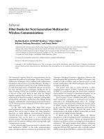
(a) (b) (c) (d) (e) (f) (g)
Figure 4: (a) All four segments of the precoded video and (b)–(g)
valid states of BRS: (b) state (0, 0), (c) state (1, 0), (d) state (1, 1), (e)
state (2, 0), (f) state (2, 1), and (g) state (2, 2).
In Figure 2, the pre-source-and-channel coded bitstream
is then passed through BRS to adjust its bit rate before being
sent to the wireless network. BRS will perform bandwidth
adaptation considering the given packet loss rate in an RD
optimized manner. The distortion here is described by the
mean square error (MSE) of the decoded video. Packet loss
rate, instead of bit error rate (BER), is considered since the
shaped precoded video will be transmitted in packets.
The decoding process (Figure 3) consists of FEC decod-
ing followed by scalable decoding. The task of rate shaping is
performed in the sender and/or midway gateways/routers.
2.2. Discrete rate-distortion optimization algorithm
BRS reduces the bit rate of each decision unit of the precoded
video before it sends the precoded video to the wireless net-

work. A decision unit can be a frame, a macroblock, and so
forth, depending on the granularity of the decision. We use a
frame as the decision unit herein. BRS performs two kinds of
RD optimizations with (i) mode decision and (ii) discrete RD
combination, depending on how much delay the rate shap-
ing decisions can allow. We will discuss both mode decision
and discrete RD combination in the following.
(a) BRS by mode decision
We consider the case in which the video is scalable coded into
two layers: one base layer and one enhancement layer. These
two layers are FEC coded with UPP. That is, the base layer
is FEC coded with stronger packet loss protection. There-
fore, there are four segments in the precoded video. The
first segment consists of the bits of the base layer video bit-
stream (upper-left segment of Figure 4a). The second seg-
ment consists of the bits of the enhancement layer video bit-
stream (upper-right segment of Figure 4a). The third seg-
ment consists of the parity bits for the base layer video bit-
stream (lower-left segment of Figure 4a). The fourth seg-
ment consists of the parity bits for the enhancement layer
video bitstream (lower-right segment of Figure 4a). BRS de-
cides a subset of the four segments to send. Note that some
constraints need to be imposed for a valid subset. For exam-
ple, if the segment that consists of the parity bits for the base
layer video bitstream is selected, the segment that consists of
the bits of the base layer video bitstream must be selected as
well. In the case of two layers of video bitstream, six valid
combinations are shown in Figures 4b, 4c, 4d, 4e, 4f, and 4g.
We call each valid combination a state. Each state is repre-
sented by a pair of integers (x, y), where x is the number of

segments selected counting from the segment consisting of
the bits of the base layer, and y is the number of segments se-
lected counting from the segment consisting of the parity bits
for the base layer. Note that x counts from the base layer be-
cause the enhancement layer cannot be decoded without the
base layer; y counts from the base layer because the base layer
needs to be protected by parity bits more than the enhance-
ment layer. The t wo integers x and y satisfy the relationship
of x ≥ y.
Each state has its RD performance represented by a dot
in the RD map, such as the ones shown in Figures 5a and
5b. The state constellations are different for different frames
because of variations in video content and packet loss rate
for different frames. If the bandwidth requirement is “B” for
each frame, BRS performs mode decision by selecting the
state that has the least distort ion. For example in Figure 5,
state (1, 1) of Frame 1 and state (2, 0) of Frame 2 are chosen.
(b) BRS by discrete RD combination
By allowing some delay in making the rate shaping decision,
BRS can optimize video streaming with a better overall qual-
ity. By allow ing some delay, we mean to accumulate the to-
tal bandwidth for a group of pictures (GOP) and to allocate
the bandwidth intelligently among frames in a GOP. Video
is typically coded with variable bit rate in order to maintain
a constant video quality. We want to al locate different num-
bers of bits for different frames in a GOP to utilize the total
bandwidth more efficiently.
Assume that there are F frames in a GOP and the total
bandwidth budget for these F frames is C.Letx(i) be the state
(represented by a pair of integers mentioned in (a)) chosen

for frame i, and let D
i,x(i)
and R
i,x(i)
be the resulting distortion
and rate allocated at frame i, respectively. The goal of the rate
shaper is to minimize
F

i=1
D
i,x(i)
(1)
subject to
F

i=1
R
i,x(i)
≤ C. (2)
FGRS for Video Streaming over Wireless Networks 179
D
00
10
20
11
21
22
B
R

(a)
D
00
10
11
20
21
22
B
R
(b)
Figure 5: RD maps of (a) Frame 1, (b) Frame 2.
D
R
(a)
D
R
a
b
c
(b)
D
m
u(m)
u(m)+1
R
m
D
n
u(n)

u(n)+1
R
n
(c)
Figure 6: Discrete RD combination algorithm: (a) and (b) elimination of states inside the convex hull of each frame, and (c) allocation of
rate to the frame m that utilizes the rate more efficiently.
The discrete RD combination algorithm [10, 17] finds
the solution by first eliminating the states that are inside the
convex hull (Figures 6a and 6b) for each frame. The algo-
rithm then allocates the rate step by step to the frame that
utilizes the rate more efficiently. That is, among frame m and
frame n,ifframem gives a better ratio than frame n regard-
ing distortion decrease over rate increase by moving from the
current state u(m) to the next state u(m) + 1, then the rate is
allocated to frame m (the next state u(m)+1 of frame m is cir-
cled in Figure 6c) from the available total bandwidth budget.
The allocation process continues until the total bandwidth
budget has been consumed completely.
3. FINE-GRAINED RATE SHAPING (FGRS)
As mentioned, BRS performs the bandwidth adaptation for
the precoded video by selecting the best state of each frame
at any given packet loss rate. Since the packet loss rate and
the bandwidth at any given time could lie in any value over
a wide range of values, we want to extend the notion of
rate shaping to allow for finer grained decisions. There then
prompts the need for source and channel coding techniques
that offer fine granularities in terms of video quality and
packet loss protection, respectively.
I B P B P
Enhancement

layer
Base layer
IBPBP
Figure 7: Dependency graph of the base layer and FGS enhance-
ment layer. Base layer has temporal prediction with P and B frames.
Enhancement layer is encoded with reference to the base layer only.
FGS has been proposed to provide bitstreams that are still
decodable when truncated at any byte interval. That is, FGS
enhancement layer bitstream is decodable at any rate pro-
vided with an intact base layer bitstream. With such a prop-
erty, FGS was adopted by MPEG-4 for streaming applications
[15]. Figure 7 illustrates two layers of video bitstream: the
base layer and the FGS enhancement layer. The base layer is
predictive coded w hile the FGS enhancement layer only uses
the corresponding base layer as the reference.
On the other h and, it has b een know n that the era-
sure codes provide “fine-grained” packet loss protection with
180 EURASIP Journal on Applied Signal Processing
more and more symbols
2
received at the FEC decoder [9, 16].
The“shaped”erasurecodeisstilldecodableifthenumber
of erasures/losses from the transmission is no more than
d
min
− 1 (number of unsent symbols), where d
min
is the min-
imum distance of the code. An erasure code can success-
fully decode the message with the number of erasures up

to d
min
− 1, considering both the unsent symbols and the
losses taken place in the transmission. Therefore, the more
symbols are sent, the better the sent bitstream can cope with
the losses. In this paper, we use Reed-Solomon codes as the
erasure codes as mentioned in Section 2. In Reed-Solomon
codes, d
min
− 1equalsn − k,wherek is the message size in
symbols and n is the code size in symbols. Thus, the partial
code with size r ≤ n is still decodable if the number of losses
from the transmission is no more than r − k.
3.1. System description of video streaming
with fine-grained rate shaping
Similar to BRS, there are three stages for transmitting the
video from the sender to the receiver: (i) precoding, (ii)
streaming with rate shaping, and (iii) decoding, as shown in
Figures 8, 9,and10.
Through MPEG-4 encoding, two layers of bitstream are
generated: one base layer and one FGS enhancement layer
(Figure 7). We will consider hereafter the bandwidth adapta-
tion and packet loss resilience for the FGS enhancement layer
bitstream only, assuming that the base layer bitstream is re-
liably transmitted as shown in Figure 9b or is considered by
approaches outside the scope of this paper. The general rule
is to perform enhancement layer bandwidth adaptation after
the base layer is reliably transmitted. The enhancement layer
bitstream will not enhance the quality of the video if its ref-
erence base layer is corrupted. Otherwise, a drift prevention

remedy is needed.
Recalling that we use a frame as the decision unit, we look
at the FGS enhancement layer bitstream of a frame. FGS en-
hancement layer bitstream consists of bits of all the bit planes
of this frame. The most significant bit plane (MSB plane) is
coded before the less significant bit planes until the least sig-
nificant bit plane (LSB plane). In a ddition, since the data in
each bit plane is variable-length coded (VLC), if some part of
a bit plane is corrupted (due to packet losses), the remaining
part of the bit plane becomes undecodable. Bits at the begin-
ning of the enhancement layer bitstream of a frame is more
important than the following bits.
Before appending the parity symbols to the FGS en-
hancement layer bitstream, we first divide all the symbols (in
this paper, each symbol consists of 14 bits) for this frame
into several sublayers (Figure 11a). The way to divide the
symbols into sublayers is arbitrary except that the later sub-
layers are longer in length than the previous ones, that is
k
1
≥ k
2
≥···≥k
h
, since we want to a chie ve UPP. A natural
way to construct the sublayers is to let Sublayer 1 consist of
2
“Symbols” are used instead of “bits” since the FEC codes use a symbol
as the encoding/decoding unit. In this paper, we use 14 bits for one sy mbol.
Theselectionofthesymbolsizeinbitsdependsontheuser.

symbols of the MSB plane, Sublayer 2 consist of symbols of
the MSB-1 plane, ,andSublayerh consist of symbols of
the LSB plane. Each sublayer is then FEC encoded with era-
sure codes to the same length n (Figure 11b). The lower por-
tions of the stripes in Figure 11b consist of the parity sym-
bols. The precoded video is stored and can be used later at
the time of delivery.
At the transport stage, FEC coded FGS bitstream is
passed through FGRS for bandwidth adaptation, given the
currentpacketlossrate.NotethatFGRSisdifferent from
JSCC-like approaches, w hich perform FEC encoding for the
FGS bitstream at the time of delivery with a bit alloca-
tion scheme that achieves certain objectives, as proposed by
Radha and van der Schaar [18, 19, 20] and Yang et al. [21].
That is, FGRS focuses on the transport aspect as opposed to
the coding aspect. Moreover, FGRS optimizes video stream-
ing r a ther than achieves certain objectives. We will elaborate
on the optimization algorithm taken later.
3.2. Fine-grained rate shaping
With the precoded video, bandwidth adaptation can be im-
plemented naively by dropping the symbols in the order
shown in Figure 12a. Given a certain bandwidth require-
ment for this frame, Sublayer 1 has more parity symbols
kept than Sublayer 2 and so on. Shaped bitstream with such
a bandw idth adaptation scheme has UPP to the sublayers.
We will refer to this method as “UPPRS” herein. However,
such UPPRS scheme might not be optimal. We propose
FGRS (Figure 12b) for bandwidth adaptation given the cur-
rent packet loss rate. The darken bars in Figure 12b are se-
lected to be sent by FGRS.

We start from the problem formulation. A FGS enhance-
ment layer bitstream provides better and better video quality
as more and more sublayers are correctly decoded. In other
words, the total distortion is decreased as more sublayers are
correctly decoded. With Sublayer 1 correctly decoded, we re-
duce the total distortion by G
1
(accumulated gain is G
1
); with
Sublayer 2 correctly decoded, we reduce the total distortion
further by G
2
(accumulated gain is G
1
+ G
2
), and so on. If
Sublayer i is corrupted, the following Sublayers i +1,i +2,
and so forth, become undecodable. Note that gain G
i
of Sub-
layer i can either ( i) be calculated, given the FGS bitstream,
after performing partial decoding; or (ii) be embedded in the
bitstream as the “metadata.” Gain G
i
of Sublayer i is different
for every frame.
Since the precoded video is transmitted over error prone
wireless networks, sublayers are subject to loss and have cer-

tain recovery rates given a particular rate shaping decision.
The expected accumulated gain is then
G =
h

i=1

G
i
i

j=1
v
j

,(3)
where h is the number of sublayers of this frame and v
j
is
the recovery rate of Sublayer j,whichisafunctionofr
j
as
will be shown later. Sublayer j is recoverable (or successfully
decodable) if the number of erasures resulting from the lossy
FGRS for Video Streaming over Wireless Networks 181
Video
FGS
encoder
FGS enhancement
layer bitstream

FEC
encoder
FEC coded FGS
enhancement layer
bitstream
Base layer
bitstream
Figure 8: System diagram of the precoding process: FGS encoding followed by FEC encoding.
Fine-grained rate
shaper (FGRS)
Fine-grained rate
shaper (FGRS)
Fine-grained rate
shaper (FGRS)
FEC coded FGS
enhancement layer
bitstream
Fine-grained rate
shaper
Wireless
network
Network conditions
(a)
Base layer
bitstream
Reliable
channel
(b)
Figure 9: Transport of the precoded bitstreams: (a) tr a nsport of the FEC coded FGS enhancement layer bitstream with rate shaper via the
wireless network and (b) transport of the base layer bitstream via the reliable channel.

Wireless
network
Shaped FGS
enhancement
layer bitstream
FEC
decoder
FGS
decoder
Reconstructed
video
Reliable
channel
Base layer
bitstream
Figure 10: System diagram of the decoding process: FEC decoding followed by FGS decoding.
Sublayer
123
···
h
(a)
Sublayer
123
···
h
(b)
Figure 11: Precoded video: (a) FGS enhancement layer bitstream
in sublayers and (b) FEC coded FGS enhancement layer bitstream.
transmission is no more than r
j

− k
j
; k
j
is the message (the
symbols from the FGS bitstream) size of Sublayer j,andr
j
is
the number of symbols selected to be sent for Sublayer j.The
recovery rate v
j
is the summation of the probabilities that no
loss occur, one erasure occurs, and so on until r
j
−k
j
erasures
occur:
v
j
=
r
j
−k
j

l=0
p{l}, j = 1 ∼ h,(4)
where l is the number of erasures that occur. If e ach erasure
occurs as a Bernoulli trial with probability e

m
, the probability
of having l erasures out of r
j
symbols is
p{l}=

r
j
l


e
m

l

1 − e
m

r
j
−l
. (5)
The symbol loss rate can be derived from the packet loss rate
as e
m
= 1 − (1 − e
p
)

m/s
,wheres is the packet size and m is the
symbol size in bits. Dep ending on the error model (Bernoulli
trial, two-state Markov model, etc.), (5)canbereplacedwith
different probability func tions.
By choosing different combinations of the number of
symbols for each sublayer, the expected accumulated gain
will be different. The rate-shaping problem can then be for-
mulated as follows: maximize
G =
h

i=1

G
i
i

j=1
v
j

(6)
182 EURASIP Journal on Applied Signal Processing
Sublayer
123 h
···
Order of dropping
(a)
Sublayer

123 h
···
(b)
Figure 12: Bandw idth adaptation with (a) UPPRS and (b) FGRS.
The part represented by darken bars are selected to be sent by FGRS.
G
r
1
r
1
+ r
2
= B
r
2
Figure 13: Intersection of the model-based hypersurface (dark sur-
face) and the bandwidth constraint (gray plane), illustrated with
h
= 2.
subject to
h

i=1
r
i
≤ B. (7)
To solve the problem, an exhausted search on all possi-
ble combinations of r = [
r
1

r
2
··· r
h
] or hill-climbing-
based approaches as described in [22, 23, 24], where RD op-
timization is made for automatic repeat request (ARQ) deci-
sions, can be performed. We propose in this paper a two-
stage RD optimization algorithm. The two-stage RD opti-
mization algorithm first finds the near-optimal solution fast.
The near-optimal solution is then refined by the hill climb-
ing approach. The proposed two-stage RD optimization is
different from [22, 23, 24] in three folds. First, the model-
based Stage 1 allows us to examine fewer samples from all
operational RD states. Only a small set of samples are needed
to train the model needed for RD optimization. Second,
the proposed distortion measure (or “expected accumulated
gain” in the terminology of the paper) accounts for the ef-
fectsofpacketlossaswellasthechannelcodesbymeans
of recovery rates. Finally, the proposed two-stage RD op-
timization algorithm can avoid the problem that the solu-
tion could be trapped in the local maximum or reach the
local maximum too slow. Due to the complexity consider-
ation, Stage 2 can be skipped. Stage 1 does not just serve as a
simple initialization stage. It can already find a near-optimal
solution.
Packetization is performed after rate shaping. That is,
symbols are grouped into packets after the decision of
r = [
r

1
r
2
··· r
h
] has been made. Similar packetization
method can be found in [20], while [25] applied bit errors
on the bitstream directly. The packets can be sent with “user
datagram protocol (UDP)” [26]. It is assumed that any error
in the packet will result in a packet loss. More considerations
on packetization can be found in UDP-Lite [27]. This pa-
per focuses on rate shaping, assuming that the network con-
dition is provided regardless of which specific packetization
method is used.
(1) Two-stage RD optimization: Stage 1
We can see from (3)and(4) that the expected accumulated
gain G is related to r = [
r
1
r
2
··· r
h
] implicitly through
the recovery rates v = [
v
1
v
2
··· v

h
]. We can instead find
a model-based hypersurface that explicitly relates r and G.
The model parameters can b e trained from a set of training
data (r, G), where r values are chosen by the user and G values
can be computed from (3)and(4). The optimal solution is in
the intersection (Figure 13) in which the model-based hyper-
surface meets the bandwidth constraint. A complex model,
with a lot of parameters, can be used to describe as close as
possible the true dist ribution of the RD states. The solution
obtained with this model will be as close to optimal as possi-
ble. However, the number of (r, G) pairs needed to train the
model-based hypersurface increases with the number of pa-
rameters.
In this paper, we use a quadratic equation to describe the
relation between r and G as follows:
ˆ
G =
h

i=1
a
i
r
2
i
+
h

i, j=1, i= j

b
ij
r
i
r
j
+
h

i=1
c
i
r
i
+ d. (8)
FGRS for Video Streaming over Wireless Networks 183
To distinguish the hypersurface modeled
ˆ
G from the real ex-
pected gain G, we denote the former with a “head” sign. The
model parameters a
i
, b
ij
, c
i
,andd are t rained differently for
each frame. They can be solved by surface fitting with a set of
training data (r, G) obtained by (3)and(4). For example, the
parameters can be computed by






a
i
’s
b
ij
’s
c
i
’s
d





=

R
T
R

−1
R
T







1
G
2
G
.
.
.
Ξ
G






,(9)
where the left super index of G is the index of the training
data and R is a matrix consisting Ξ rows of (r
2
i
’s, r
i
r
j
’s, r

i
’s, 1).
The complexity of computing a
i
’s, b
ij
’s, c
i
’s, and d relates
to the number of parameters h
2
+ h + 1 and the number of
training data Ξ, using (9). Note that the number of train-
ing data Ξ is in general much greater than the number of
parameters h
2
+ h + 1. Thus, a more complex model, such
as a third-order model with h
3
+ h
2
+ h +1parameters,is
not suitable since it requires much more training data than a
quadratic model. In addition, second-order Taylor expansion
can nicely approximate most functions. Equation (8)can
be seen as a second-order approximation to (3). To reduce
the computation complexity in realit y, we can also choose a
smaller h if the precoding process is also under our control
(which is outside the scope of the rate shaper).
With (8), the near-optimal solution can be obtained by

the use of Lagrange multiplier as fol lows:
J =

h

i=1
a
i
r
2
i
+
h

i, j=1, i= j
b
ij
r
i
r
j
+
h

i=1
c
i
r
i
+ d


+ λ

h

i=1
r
i
− B

.
(10)
By ∂J/∂r
i
= 0, we get
r
i
=
−1
2a
i


h

j=1, j=i
b
ij
r
j

+ c
i
+ λ


, (11)
where
λ =
2B +

h
i=1

1/a
i



h
j=1, j=i
b
ij
r
j
+ c
i

−

h

i=1

1/a
i

. (12)
The near-optimal solution can be solved recursively using
(11)and(12), starting from the initial condition that all sub-
layers are allocated with equal number of symbols, r
1
= r
2
=
···=r
h
= B/h.
(2) Two-stage RD optimization: Stage 2
Stage 1 of the two-stage RD optimization gives a near-
optimal solution. The solution can be refined by a hill-
climbing-based approach (Algorithm 1). The solution from
Stage1isperturbedinStage2inordertoyieldalargerex-
While (stop == false)
z
i
= r
i
for all i = 1 ∼ h
For ( j = 1; j<= h; j ++)
For (k = 1; k<= h; k ++)
z

k
= z
k
+deltafork == j //Increase sublayer j
z
k
= z
k
− delta /(h − 1) for k! = j //Decrease others
End
Evaluate G
j
End
Find the j

with the largest G
j

.
For (i = 1; i<= h; i ++)
r
i
= r
i
+deltafori == j

r
i
= r
i

− delta /(h − 1) for i! = j

End
Calculate the stop criter ion.
End
Algorithm 1: Pseudocodes of hill-climbing algorithm.
1 − p
Good
p
q
1 − q
Bad
Figure 14: Two-state Markov chain for bit error simulation.
e
b
= 10
−4
1
0.8
0.6
0.4
0.2
0
Packet loss rate (e
p
)
0.03
0.02
0.01
0

Transition probability (
p
)
0
20
40
60
80
100
Packet size in bits (
s
)
Figure 15: Packet loss rate as a function of the transition probability
and the packet size.
pected accumulated gain. The process can be iterated until
the solution reaches a stopping criterion such as the conver-
gence.
The idea of allocating bandwidth optimally for sublayers
canbeextendedtoahigherleveltoallocatebandwidtheffi-
ciently among frames in a GOP. The problem formulation is
184 EURASIP Journal on Applied Signal Processing
14000
12000
10000
8000
6000
4000
2000
0
Bandwidth (bps)

1591317212529
Time index
0.2
0.18
0.16
0.14
0.12
0.1
0.08
0.06
0.04
0.02
0
Packet loss rate
Bandwidth
Packet loss rate
Figure 16: Network conditions: bandwidth and packet loss r ate
fluctuations.
slightly different from the original (6) as follows: maximize
G =
F

m=1

h

i=1

G
mi

i

j=1
v
mj

(13)
subject to
F

m=1
h

i=1
r
mi
≤ C, (14)
where F is the number of frames in a GOP. FGRS will incur
delay with duration of F frames if it allows for optimization
among frames in a GOP.
To summarize, the proposed FGRS achieves the best
streaming performance for FEC coded FGS bitstream with
the two-stage RD optimization. The two-stage RD opti-
mization obtains the optimal solution by first finding the
near-optimal solution, then refining the solution with a hill-
climbing-based approach.
4. EXPERIMENT
We start by describing the wireless network simulation for
the experiment. We then compare the proposed FGRS with
the naive UPPRS described in Figure 12a.

4.1. Experiment setup
Wireless networks are generally associated with time-varying
packet loss r a te and fluctuating bandwidth. The packet loss
rate and bandw idth vary at each time interval. We simulate
random bandwidth fluctuation according to an autoregres-
sive (AR) process [28] and use a two-state Markov model
[29, 30] to simulate the bursty bit errors. The two-state
Markov model is also adopted by [31, 32]. “Good” and “Bad”
in Figure 14 correspond to error free and erroneous states
ofabit,respectively.TheBERe
b
is related to the transition
probabilities p and q by e
b
= p/(p + q).
Since the coded bitstream is transmitted in packets, let us
look at how the packet loss rate e
p
relates to the transition
Table 1: PSNR gains in Y, U, and V components with sequences
Akiyo, Foreman, and Stefan.
PSNR gain (dB) Y component U component V component
Akiyo 1.38 1.28 0.87
Foreman 0.86 0.44 0.52
Stefan 0.76 0.34 0.38
probability p and the BER e
b
.WithBERe
b
, transition prob-

ability p, and packet size s, the packet loss rate of the s-bit
packet is
e
p
= 1 −

1 − e
b

(1 − p)
s−1
. (15)
We observe two properties from (15) given the same BER
e
b
: (i) the smaller the transition probability p, the smaller
the packet loss rate e
p
, and (ii) the smaller the packet size s,
the smaller the packet loss rate e
p
. These two properties are
shown in Figure 15 with e
b
= 10
−4
.
Besides the two properties we have just seen, it is also
known that to detect the loss of packets, some information
such as the packet number has to be added to each packet.

The smaller the packet is, the heavier the overhead is. There-
fore,itisatrade-off between the selec tion of the packet size
and the resulting packet loss rate. We use s = 280 (bits) in
this paper. Users can select the packet size s according to real
system consideration using (15).
The time-varying bandwidth is simulated pseudoran-
domly according to an AR process. The bandwidth available
at current time t is fed to FGRS optimization of time t +1in
order to simulate the delay nature of the network feedback.
Such delay in feedback will not affect too much the perfor-
mance since the bandwidth requirements of the two consec-
utive frames are closely related, given the AR assumption. Ex-
ample traces of simulated packet loss rate and bandwidth ob-
served at the rate shaper are shown in Figure 16.Thepacket
loss rate is plotted using the line and the bandwidth is illus-
trated using the vertical bars. Each interval in the axis of time
index represents 0.33 seconds.
The test video sequences are “Akiyo,” “Foreman,” and
“Stefan” in common intermediate format (CIF) (Figures 17a,
17b,and17c). The frame rate is three frames/s.
4.2. Experiment result
Results for sequence Akiyo are shown in Figures 18 and 19.
Results for sequence Foreman is shown in Figures 20 and
21. Results for sequence Stefan is shown in Figures 22 and
23. The overall PSNR performance for all the three test se-
quences are listed in Figure 24 and Ta ble 1. Results for differ-
ent wireless channel conditions are shown in Figure 25.
Figures 18, 20,and22 show how bit allocation with UP-
PRS and FGRS is done in bytes (converted from number of
symbols) for each sublayer. After bit allocation, the number

of symbols to send is constrained to b e at least k
i
for each
sublayer (i.e., to satisfy r
i
≥ k
i
) by moving the number of
symbols allocated for the higher sublayers to the lower layers
that does not satisfy r
i
≥ k
i
as shown in Algorithm 2.
FGRS for Video Streaming over Wireless Networks 185
(a) (b) (c)
Figure 17: Test video sequences in CIF: (a) Akiyo, (b) Foreman, and (c) Stefan.
4500
3600
2700
1800
900
0
Byte allocations
1591317212529
Frame number
Sub 10
Sub 9
Sub 8
Sub 7

Sub 6
Sub 5
Sub 4
Sub 3
Sub 2
Sub 1
(a)
4500
3600
2700
1800
900
0
Byte allocations
1 5 9 1317212529
Frame number
Sub 10
Sub 9
Sub 8
Sub 7
Sub 6
Sub 5
Sub 4
Sub 3
Sub 2
Sub 1
(b)
Figure 18: Sublayer byte allocations with sequence Akiyo by (a) UPPRS and (b) FGRS.
With limited bandwidth, FGRS allocates enough bytes to
Sublayer 1 (indicated as sub 1 in the figures) first, than to

Sublayer 2, and so on. Allocating enough bytes to a sublayer
means providing enough packet loss protection, but not al-
locating too many bytes as to include too much redundancy.
The bit allocation process happens automatically by the pro-
posed two-stage RD optimization, considering the current
packet loss rate and the bandwidth requirement.
From the frame-by-frame PSNR performance in Fig-
ures 19, 21,and23, we see that the proposed FGRS pro-
vides superior results to UPPRS. Comparing performance
with different sequences, the PSNR improvement of FGRS
over UPPRS is the most significant in sequence Akiyo, fol-
lowed by sequence Foreman and Stefan. Sequence Stefan is
the most challenging one with the most complex scene and
the highest motion. The source coding rates of the FGS en-
hancement layer bitstream of Akiyo, Foreman, and Stefan are
354.69 kbps, 747.74 kbps, and 975.70 kbps. Hence, given the
same amount of bits allocated by FGRS, the PSNR of se-
quence Stefan is the smallest among the three. Considering
the gain in the Y component, FGRS yields 0.76 dB to 1.38 dB
improvement compared to UPPRS as shown in Table 1.
To validate the performance of the proposed algorithm,
the performance in terms of the overall PSNR of the Y com-
ponents at various wireless channel conditions is shown in
Figure 25, where we consider a two-state Markov model a t
various speeds and SNRs [29]. Figure 25a shows the 3D plots
of the overall PSNR. At all wireless channel conditions, FGRS
outperforms UPPRS.
Figure 25b shows the overall PSNR at v arious speeds at
SNR
= 10 dB. Fixed SNR value gives the same BER of the

wireless channel. The higher the speed is, the more bursty the
bit error of the wireless channel is. In other words, the larger
the transition probability is. From the results, we see that the
PSNR drops as the speed increases. The higher the transi-
tion probability is, the higher the packet loss rate is, given
186 EURASIP Journal on Applied Signal Processing
39
38
37
36
35
34
33
32
PSNR (dB)
0 5 10 15 20 25 30
Frame number
UPPRS
FGRS
(a)
43
42
41
40
39
38
37
PSNR (dB)
0 5 10 15 20 25 30
Frame number

UPPRS
FGRS
(b)
44
43
42
41
40
PSNR (dB)
0 5 10 15 20 25 30
Frame number
UPPRS
FGRS
(c)
Figure 19: Frame-by-frame PSNR of UPPRS and FGRS with se-
quence Akiyo: (a) PSNR of the Y component, (b) PSNR of the U
component, and (c) PSNR of the V component.
the same BER. Higher packet loss rate has the effect of re-
quiring more parity bits in the shaped bitstream, and higher
4500
3600
2700
1800
900
0
Byte allocations
1591317212529
Frame number
Sub 10
Sub 9

Sub 8
Sub 7
Sub 6
Sub 5
Sub 4
Sub 3
Sub 2
Sub 1
(a)
4500
3600
2700
1800
900
0
Byte allocations
1591317212529
Frame number
Sub 10
Sub 9
Sub 8
Sub 7
Sub 6
Sub 5
Sub 4
Sub 3
Sub 2
Sub 1
(b)
Figure 20: Sublayer byte allocations with sequence Foreman by (a)

UPPRS and (b) FGRS.
probability of corrupting the packets that carries the shaped
bitstream, thus, the PSNR value is lower.
Figure 25c shows the overall PSNR at various SNRs at
speed = 10 km/h. Fixed speed gives the same burstiness of
the bit errors of the wireless channel. The larger the SNR is,
the smaller the BER is. We see from the results that the PSNR
value increases with SNR. Smaller packet loss rate then leads
to a higher PSNR.
Optimization for video streaming needs to be real time.
As mentioned, in the training process for the model-based
hypersurface, only a few number of operational RD states
need to be examined, which saves the time. Thus, the two-
stage RD optimization is preferred over the hill-climbing-
based approach. In addition, as mentioned in Section 3.2,
Step 2 can be skipped without too much performance degra-
dation.
FGRS for Video Streaming over Wireless Networks 187
34
32
30
28
26
PSNR (dB)
0 5 10 15 20 25 30
Frame number
UPPRS
FGRS
(a)
40

39
38
37
36
35
34
PSNR (dB)
0 5 10 15 20 25 30
Frame number
UPPRS
FGRS
(b)
42
41
40
39
38
37
36
35
34
PSNR (dB)
0 5 10 15 20 25 30
Frame number
UPPRS
FGRS
(c)
Figure 21: Frame-by-frame PSNR of UPPRS and FGRS with se-
quence Foreman: (a) PSNR of the Y component, (b) PSNR of the U
component, and (c) PSNR of the V component.

5. CONCLUSION
We proposed in this paper a novel FGRS approach to per-
form bandwidth adaptation for the precoded video, which
4500
3600
2700
1800
900
0
Byte allocations
1591317212529
Frame number
Sub 10
Sub 9
Sub 8
Sub 7
Sub 6
Sub 5
Sub 4
Sub 3
Sub 2
Sub 1
(a)
4500
3600
2700
1800
900
0
Byte allocations

1591317212529
Frame number
Sub 10
Sub 9
Sub 8
Sub 7
Sub 6
Sub 5
Sub 4
Sub 3
Sub 2
Sub 1
(b)
Figure 22: Sublayer byte allocations with sequence Stefan by (a)
UPPRS and (b) FGRS.
is both FGS coded and FEC coded. FGRS utilizes the fine
granularity property of FGS and FEC. Moreover, FGRS op-
timizes video streaming rather than achieves heuristic ob-
jectives. A two-stage rate-distortion (RD) optimization al-
gorithm is used. The two-stage RD optimization algorithm
finds the solution efficiently. The proposed FGRS outper-
forms UPPRS.
The novelty of the paper lies in three aspects. Although
FGS has been proposed to provide fine granularity for pre-
compressed video, none of the prior works has shown how
to adapt the rate of the FGS bitstream that is protected by
the FEC codes. Note that related work performs FEC en-
coding for the FGS bitstream at the time of delivery. Sec-
ondly, we formulate the FGRS problem as an RD optimiza-
tion problem, while the work by van der Schaar and Radha

[20] is not optimized but to achieve a certain target recov-
ery rate. In addition, the distortion measure, which is called
188 EURASIP Journal on Applied Signal Processing
31
30
29
28
27
26
25
24
PSNR (dB)
0 5 10 15 20 25 30
Frame number
UPPRS
FGRS
(a)
36
35
34
33
32
31
30
PSNR (dB)
0 5 10 15 20 25 30
Frame number
UPPRS
FGRS
(b)

36
35
34
33
32
31
30
29
PSNR (dB)
0 5 10 15 20 25 30
Frame number
UPPRS
FGRS
(c)
Figure 23: Frame-by-frame PSNR of UPPRS and FGRS with se-
quence Stefan: (a) PSNR of the Y component, (b) PSNR of the U
component, and (c) PSNR of the V component.
36
34
32
30
28
26
PSNR (dB)
Akiyo Foreman Stefan
Sequence
UPPRS
FGRS
(a)
42

40
38
36
34
32
30
PSNR (dB)
Akiyo Foreman Stefan
Sequence
UPPRS
FGRS
(b)
43
41
39
37
35
33
31
PSNR (dB)
Akiyo Foreman Stefan
Sequence
UPPRS
FGRS
(c)
Figure 24: Overall PSNR of UPPRS and FGRS with sequences
Akiyo, Foreman, and Stefan: (a) PSNR of the Y component, (b)
PSNR of the U component, and (c) PSNR of the V component.
FGRS for Video Streaming over Wireless Networks 189
42

41
40
39
38
37
36
35
34
33
PSNR (dB)
20
18
16
14
12
10
SNR (dB)
2
4
6
8
10
Speed (km/h)
UPPRS
FGRS
(a)
42
41
40
39

38
37
36
35
34
33
PSNR (dB)
2345678910
Speed (km/h)
UPPRS
FGRS
(b)
40
39
38
37
36
35
34
33
PSNR (dB)
2345678910
SNR (dB)
UPPRS
FGRS
(c)
Figure 25: Performance (PSNR of the Y component) of all methods
at various wireless channel conditions for sequence Foreman: (a)
3D view of PSNR at various speeds and SNRs; (b) PSNR at various
speeds; (c) PSNR at various SNRs.

For (i = 1; i<= h; i ++)
If r
i
<k
i
a = k
i
− r
i
//the difference needed to satisfy r
i
>k
i
b = c = 0
For ( j = h; j>= 1&c<a; j −−)
b = r
j
>a? a : r
j
//the symbols got from Sublayer j
c+ = b
r
j
−=b
End
r
i
= k
i
End

End
Algorithm 2: Pseudocodes satisfying r
i
≥ k
i
after bit allocation.
“gain” in the paper, is derived from the current packet loss
rate in addition to the video characteristics. The gain is de-
fined as the expected gain given the current packet loss rate.
Prior work of DRS defines the distortion measure solely from
the video characteristics. Thirdly, the RD optimization prob-
lem is solved by the proposed two-stage RD optimization al-
gorithm, which can a chieve the optimal solution fast. It is
crucial that optimization for video streaming is done in real
time.
Future work includes considering the smoothness crite-
rion in FGRS optimization such as [33] to smooth the fluc-
tuating PSNR resulted from the time-varying network con-
ditions. Such fluctuation is not inherent from the FGRS al-
gorithm. We can also investigate more the effect of outdated
network information on FGRS, in addition to the simulation
done in this paper by delaying the network bandwidth feed-
back. Moreover, deploying FGRS in a large network system,
such as the “end system multicast (ESM)” [34]system,can
be an exciting future research direction.
ACKNOWLEDGMENTS
This work was supported in part by Industrial Technology
Research Institute. The authors would like to acknowledge
the suggestions of Professor Mihaela van der Schaar, Univer-
sity of California at Davis, Professor Jose Moura and Profes-

sor Rohit Negi, Carnegie Mellon University, Professor Alex
Eleftheriadis and Professor Shih-Fu Chang, Columbia Uni-
versity, Professor Antonio Ortega, University of Southern
California, and the reviewers of the paper.
REFERENCES
[1] Y. Wang, S. Wenger, J. Wen, and A. K. Katsaggelos, “Error re-
silient video coding techniques,” IEEE Signal Processing Mag-
azine, vol. 17, no. 4, pp. 61–82, 2000.
[2] J. Cabrera, A. Ortega, and J. I. Ronda, “Stochastic rate-control
of video coders for wireless channels,” IEEE Trans. Circuits
and Systems for Video Technology, vol. 12, no. 6, pp. 496–510,
2002.
190 EURASIP Journal on Applied Signal Processing
[3] Z. He, J. Cai, and C. W. Chen, “Joint source channel rate-
distortion analysis for adaptive mode selection and rate con-
trol in wireless video coding,” IEEE Trans. Circuits and Systems
for Video Technology, vol. 12, no. 6, pp. 511–523, 2002.
[4] G. Cheung and A . Zakhor, “Bit allocation for joint source/
channel coding of scalable video,” IEEE Trans. Image Process.,
vol. 9, no. 3, pp. 340–356, 2000.
[5] L. P. Kondi, F. Ishtiaq, and A. K. Katsaggelos, “Joint source-
channel coding for motion-compensated DCT-based SNR
scalable video,” IEEE Trans. Image Process.,vol.11,no.9,pp.
1043–1052, 2002.
[6] A. Eleftheriadis and D. Anastassiou, “Meeting arbitrary
QoS constraints using dynamic rate shaping of coded digi-
tal video,” in Proc. 5th International Workshop on Networking
and Operating System Support for Digital Audio and Video,pp.
95–106, Durham, NH, USA, April 1995.
[7] W. Zeng and B. Liu, “Rate shaping by block dropping for

transmission of MPEG-precoded video over channels of dy-
namic bandwidth,” in Proc. 4th ACM International Conference
on Multimedia, pp. 385–393, Boston, Mass, USA, November
1996.
[8] S. Jacobs and A. Eleftheriadis, “Streaming video using dy-
namic rate shaping and TCP congestion control,” Journal of
Visual Communication and Image Representation, vol. 9, no. 3,
pp. 211–222, 1998.
[9] S. Wicker, Error Control Systems for Digital Communication
and Storage, Prentice Hall, Englewood Cliffs, NJ, USA, 1995.
[10] T. P C. Chen and T. Chen, “Adaptive joint source-channel
coding using rate shaping,” in Proc. IEEE Int. Conf. Acoustics,
Speech, Sig nal Processing, Orlando, Fla, USA, May 2002.
[11] D. S. Turaga and T. Chen, “Fundamentals of video compres-
sion: H.263 as an example,” in Compressed Video over Net-
works, M T. Sun and A. R. Reibman, Eds., pp. 3–34, Marcel
Dekker, NY, USA, 2001.
[12] B. G. Haskell, A. Puri, and A. N. Netravali, Digital Video: An
Introduction to MPEG-2, Chapman & Hall, NY, USA, 1997.
[13] Motion Pictures Experts Group, “Overview of the MPEG-4
standard,” ISO/IEC JTC 1/SC 29/WG 11 N 2459, 1998.
[14] J. Hagenauer, “Rate-compatible punctured convolutional
codes (RCPC codes) and their applications,” IEEE Trans.
Communications, vol. 36, no. 4, pp. 389–400, 1988.
[15] W. Li, “Overview of fine granularity scalability in MPEG-4
video standard,” IEEE Trans. Circuits and Systems for Video
Technology, vol. 11, no. 3, pp. 301–317, 2001.
[16] L. Rizzo, “Effective erasure codes for reliable computer com-
munication protocols,” ACM Computer Communication Re-
view, vol. 27, no. 2, pp. 24–36, 1997.

[17] A. Ortega and K. Ramchandran, “Rate-distortion methods
for image and video compression,” IEEE Signal Processing
Magazine, vol. 15, no. 6, pp. 23–50, 1998.
[18] H. M. Radha, M. van der Schaar, and Y. Chen, “The MPEG-
4 fine-grained scalable video coding method for multimedia
streaming over IP,” IEEE Trans. Multimedia,vol.3,no.1,pp.
53–68, 2001.
[19] M. van der Schaar and H. M. Radha, “A hybrid temporal-SNR
fine-granular scalability for internet video,” IEEE Trans. Cir-
cuits and Systems for Video Technology, vol. 11, no. 3, pp. 318–
331, 2001.
[20] M. van der Schaar and H. M. Radha, “Unequal packet loss re-
silience for fine-granular-scalability video,” IEEE Trans. Mul-
timedia, vol. 3, no. 4, pp. 381–394, 2001.
[21] X. K. Yang, C. Zhu, Z. G. Li, G. N. Feng, S. Wu, and N. Ling, “A
degressive error protection algorithm for MPEG-4 FGS video
streaming,” in Proc. 2002 IEEE International Conference on
Image Processing, pp. 737–740, Rochester, NY, USA, Septem-
ber 2002.
[22] A. E. Mohr, E. A. Riskin, and R. E. Ladner, “Unequal loss pro-
tection: graceful degradation of image quality over packet era-
sure channels through forward error correction,” IEEE Jour-
nal on Selected Areas in Communications,vol.18,no.6,pp.
819–828, 2000.
[23] P. A. Chou and Z. Miao, “Rate-distortion optimized stream-
ing of packetized media,” submitted to IEEE Trans. Multime-
dia.
[24] J. Chakareski, P. A. Chou, and B. Aazhang, “Computing rate-
distortion optimized policies for streaming media to wire-
less clients,” in Proc. D ata Compression Conference, Snowbird,

Utah, USA, April 2002.
[25] G. Cote, S. Shir ani, and F. Kossentini, “Optimal mode selec-
tion and synchronization for robust video communications
over error-prone networks,” IEEE Journal on Selected Areas in
Communications, vol. 18, no. 6, pp. 952–965, 2000.
[26] J. Postel, “User datagram protocol (RFC 768),” Internet En-
gineering Task Force, Internet draft, RFC-768, August, 1980,
/>[27] L A. Larzon, M. Degermark , and S. Pink, “Efficient use of
wireless bandwidth for multimedia applications,” in Proc.
6th IEEE International Workshop on Mobile Multimedia Com-
munications, pp. 187–193, San Diego, Calif, USA, November
1999.
[28] A. J. Ganesh, “Estimating effective bandwidths from traffic
data,” in Proc. IEEE Conference on Global Communications,
pp. 654–658, London, UK, November 1996.
[29] J P. Ebert and A. Willig, “A Gilbert-Elliot bit error model
and the efficient use in packet level simulation,” Tech. Rep.
TKN-99-002, Telecommunication Networks Group, Techni-
cal University of Berlin, Berlin, 1999.
[30] M. Yajnik, S. Moon, J. Kurose, and D. Towsley, “Measurement
and modeling of the temporal dependence in packet loss,” in
18th Annual Joint Conference of the I EEE Computer and Com-
munications Societies, pp. 345–352, NY, USA, March 1999.
[31]S.A.Khayam,S.S.Karande,M.Krappel,andH.M.Radha,
“Cross-layer protocol design for real-time multimedia appli-
cations over 802.11b networks,” in IEEE 2003 International
Conference on Multimedia and Expo, pp. 425–428, Baltimore,
Md, USA, July 2003.
[32] F. Yang, Q. Zhang, W. Zhu, and Y Q. Zhang, “An end-to-end
TCP-friendly streaming protocol for multimedia over wireless

internet,” in IEEE 2003 International Conference on Multime-
dia and Expo, pp. 429–432, Baltimore, Md, USA, July 2003.
[33] X. M. Zhang, A. Vetro, Y. Q. Shi, and H. Sun, “Constant qual-
ity constrained rate allocation for FGS coded video,” IEEE
Trans. Circuits and Systems for Video Technology, vol. 13, no.
2, pp. 121–130, 2003.
[34]Y H.Chu,S.G.Rao,S.Seshan,andH.Zhang, “Acasefor
end system multicast,” IEEE Journal on Selected Areas in Com-
munications, vol. 20, no. 8, pp. 1456–1471, 2002.
Trista Pei-chun Chen received her B.S.
and M.S. degrees from National Tsing
Hua University, Hsinchu, Taiwan, in 1997
and 1999, respectively, and her Ph.D. de-
gree in electrical and computer engineer-
ing from Carnegie Mellon University, Pitts-
burgh, Pennsylvania, in 2003. Trista is cur-
rently a video architect at NVIDIA Corpo-
ration, Santa Clara, California, performing
design and testing of video hardware. From
July 1998 to June 1999, she was a software engineer developing fin-
gerprint identification algorithms at Startek Engineering Incorpo-
rated, Hsinchu, Taiwan. During the summer of 2000, she was with
FGRS for Video Streaming over Wireless Networks 191
HP Cambridge Research Laboratory, Cambridge, Massachusetts,
conducting a research in image retrieval for massive databases.
During the summer of 2001, she was with Pittsburg h Sony De-
sign Center, Pittsburgh, Pennsylvania, designing circuits for video
watermarking (VWM). Her research interests include multimedia
hardware, networked video, watermar k/data hiding, image pro-
cessing, and biometric signal processing. She is a Member of the

IEEE.
Tsuhan Chen has been with the Depart-
ment of Electrical and Computer Engi-
neering, Carnegie Mellon University, Pitts-
burgh, Pennsylvania since October 1997,
where he is now a Professor. He directs the
Advanced Multimedia Processing Labora-
tory. His research interests include multi-
media signal processing and communica-
tion, audio-visual interaction, biometrics,
processing of 2D/3D graphics, bioinformat-
ics, and building collaborative virtual environments. From Au-
gust 1993 to October 1997, he worked in the Visual Communi-
cations Research Department, AT&T Bell Laboratories, Holmdel,
New Jersey, and later at AT&T Labs-Research, Red Bank, New Jer-
sey. Tsuhan helped create the Technical Committee on Multime-
dia Signal Processing, as the Founding Chair, and the Multimedia
Signal Processing Workshop, both in the IEEE Signal Processing
Society. He has recently been appointed as the Editor-in-Chief for
IEEE Transactions on Multimedia for 2002–2004. He has coedited
a book, Advances in Multimedia: Systems, Standards, and Networks.
Tsuhan received the B.S. degree in electrical engineering from the
National Taiwan University in 1987, and the M.S. and Ph.D. degrees
in electrical engineering from the California Institute of Technol-
ogy, Pasadena, California, in 1990 and 1993, respectively. He is a
recipient of the National Science Foundation CAREER Award.