Báo cáo hóa học: " Watermarking Algorithms for 3D NURBS Graphic Data" pot
Bạn đang xem bản rút gọn của tài liệu. Xem và tải ngay bản đầy đủ của tài liệu tại đây (1.14 MB, 11 trang )
EURASIP Journal on Applied Signal Processing 2004:14, 2142–2152
c
2004 Hindawi Publishing Corporation
Watermarking Algorithms for 3D NURBS Graphic Data
Jae Jun Lee
Institute of New Media and Communications (INMC), School of Elect rical Engineering,
Seoul National University, Seoul 151-744, Korea
Email:
NamIkCho
Institute of New Media and Communications (INMC), School of Elect rical Engineering,
Seoul National University, Seoul 151-744, Korea
Email:
Sang Uk Lee
Institute of New Media and Communications (INMC), School of Elect rical Engineering,
Seoul National University, Seoul 151-744, Korea
Email:
Received 14 March 2003; Revised 10 June 2004
Two watermarking algorithms for 3D nonuniform rational B-spline (NURBS) graphic data are proposed: one is appropriate for
the steganography, and the other for watermarking. Instead of directly embedding data into the parameters of NURBS, the pro-
posed algorithms embed data into the 2D virtual images extra cted by parameter sampling of 3D model. As a result, the proposed
steganography algorithm can embed information into more places of the surface than the conventional algorithm, while preserv-
ing the data size of the model. Also, any existing 2D watermarking technique can be used for the watermar king of 3D NURBS
surfaces. From the experiment, it is found that the algorithm for the watermarking is robust to the attacks on weights, control
points, and knots. It is also found to be robust to the remodeling of NURBS models.
Keywords and phrases: watermark, 3D image, nonunifor m rational B-spline (NURBS), steganography, data hiding.
1. INTRODUCTION
With the development of computing environments, 3D
models became widely used and are being produced in
great numbers. 3D models are usually represented by mesh,
nonuniform rational B-spline (NURBS), or voxel. Among
these models, mesh is quite widely used because many studies
on the mesh have already been performed, and also because
the scanned 3D data are naturally the sampling points of sur-
faces. However, the mesh representation has drawbacks in
that it requires large amount of data, and it cannot represent
mathematically rigorous curves and surfaces. Unlike mesh,
the NURBS describes 3D models by using mathematical for-
mula. The data size for the NURBS is remarkably smaller
than that for the mesh because the surface can be represented
by only a few parameters. Also, the NURBS is smooth in na-
ture so that the smoothness of NURBS is restricted only by
hardware resolution. Hence, the NURBS is used in CAD and
other areas which need high precision, and it is also used in
animation because the motion of an object can be realized by
successively adjusting some of the parameters.
Although the amount of 3D multimedia data is dramat-
ically increasing, there has not been much discussion on the
watermarking of 3D models, especially on the 3D NURBS
models. For example, Ohbuchi et al. proposed an algorithm
that embeds information into the knot equations by knot
reparameterization [1]. This algorithm has merits that the re-
sulting NURBS model has exactly the same shape as the orig-
inal one, and that the number of knots and control points
are also unchanged. But the embedded information can be
detected only when one has the original model because it is
embedded into the coefficients of the function that reparam-
eterizes the original knot vector. Moreover, the maximum
number of embedded data is only three, which is the degree
of freedom of bilinear function, and a slight modification of
the knots and control points makes it impossible to detect
the information.
In this paper, we propose two watermarking algorithms
for 3D NURBS, one is suitable for the steganography (for se-
cret communication between trusting parties) and the other
for the robust watermarking. In the proposed algorithm, a
virtual NURBS model is first generated from the original
Watermarking Algorithms for 3D NURBS Graphic Data 2143
one. Instead of embedding information into the parameters
of NURBS data as in the existing algorithm, the proposed
algorithms extract several 2D images from the 3D virtual
model and apply the 2D watermarking methods.
In the steganography algorithm, 3D virtual model is first
sampled in each of u and v directions, where u and v are pa-
rameters of NURBS. That is, a sequence of {u, v} is gener-
ated, where the number of elements is limited to be less than
that of control points. Then, three 2D virtual images are ex-
tracted, the pixels of which are the distances from the sample
points to the x, y,andz plane, respectively. The watermark
is embedded into these 2D images, which leads to the mod-
ification of control points of NURBS. As a result, the origi-
nal model is changed by the watermark data as much as the
quantity of embedded data. But the data size of the NURBS
model is preserved because there is no change in the num-
ber of knots and control points. For the extraction of em-
bedded information, modified virtual sample points are first
acquired by the matrix operation of basis functions in accor-
dance with the {u, v} sequence. Even if the third party has
the original NURBS model, the embedded information can-
not be acquired without {u, v} sequence as a key, which is a
good property for the steganography.
The second algorithm is suitable for the robust water-
marking. This algorithm also samples the 3D virtual model.
But the difference from the steganography algorithm is that
the number of sampled points is not limited by the num-
ber of control points of the original NURBS model. Instead,
the sequence
{u, v} is chosen so that the sampling interval
in the physical space is kept constant. This makes the model
robust against the attacks on knot vectors, such as knot in-
sertion, removal, and so forth. The procedure of making 2D
virtual images is the same as the steganography algorithm.
Then, the watermarking algorithms for 2D images are ap-
plied to these virtual images, and a new NURBS model is
made by the approximation of watermarked sample points.
The watermarks in the coordinate of each sample point are
distorted within the error bound by approximation. But such
distortion can be controlled by the strength of embedded wa-
termarks and the magnitude of error bound. Since the points
are not sampled in the physical space (x-,y-,z-coordinate)
but in the parametric space (u-,v-coordinate), the proposed
algorithm for watermarking is also found to be robust against
the attacks on the control points that determine the model’s
transition, rotation, scaling, and projection. A preliminary
version of this paper has appeared in [2].
This paper is organized as follows. In Section 2, the
NURBS model is briefly reviewed. In Section 3, the water-
marking applications considered are introduced and the pro-
posed algorithms are described. Implementation of the algo-
rithms and experimental results are presented in Section 4,
followed by Section 5 presenting some conclusions.
2. NURBS CURVES AND SURFACES
For the explanation of the proposed algorithms in later sec-
tions, we first briefly review the definition and notation of
NURBS. More details on the NURBS can be found in [3, 4].
A NURBS surface S(u, v) = (x(u, v), y(u, v), z(u, v)) of
degree p in the u direction and degree q in the v direction is
defined by a bivariate function of the form
S(u, v) =
n
i=0
m
j=0
R
i, j
(u, v)P
i, j
,(1)
where
R
i, j
(u, v) =
N
i,p
(u)N
j,q
(v)w
i, j
n
k=0
m
l=0
N
k,p
(u)N
l,q
(v)w
k,l
. (2)
In (1), {P
ij
} form a bidirectional control net, and {w
i
} in (2)
are the weights. {N
i,p
(u)} are the ith B-spline basis function
of degree p, which can be defined recursively as
N
i,0
(u) =
1ifu
i
≤ u<u
i+1
,
0 otherwise,
N
i,p
(u) =
u − u
i
u
i+p
− ui
N
i,p−1
(u)
+
u
i+p+1
− u
u
i+p+1
− u
i+1
N
i+1,p−1
(u)
(3)
on a nonperiodic and nonuniform knot vector
U =
a, , a
p+1
, u
p+1
, , u
r−p−1
, b, , b
p+1
,(4)
where u
i
≤ u
i+1
, i = 0, , r − 1, and r = n + p +1.{N
j,q
(v)}
are analogously defined as {N
i,p
(u)}.
The equation for the NURBS curve can be derived from
the surface of (1) by fixing one of the variables u or v.Tobe
precise, isoparametric curves C
u
0
(v)andC
v
0
(u)ofNURBS
surface S(u, v) trace the trajectory curve for the fixed u
0
and
v
0
, respectively, and they intersect at a surface point S(u
0
, v
0
).
For the simplicity of explanation, all the weights are set to
one. Then C
u
0
(v)isdefinedas
C
u
0
(v) = S
u
0
, v
w
i,j
=1, ∀i, j
=
m
j=0
N
j,q
(v)
n
i=0
N
i,p
u
0
P
i, j
=
m
j=0
N
j,q
(v)Q
j
u
0
,
(5)
where
Q
j
u
0
=
n
i=0
N
i,p
u
0
P
i, j
. (6)
Analogously
C
v
0
(u) =
n
i=0
N
i,p
(u)Q
i
v
0
,(7)
where
Q
i
v
0
=
m
j=0
N
j,q
v
0
P
i, j
. (8)
2144 EURASIP Journal on Applied Signal Processing
Watermarks
Watermark
embedding
2D virtual
images
NURBS
sampling
Parameter
sequences
Watermarke d
2D virtual
images
Virtual
NURBS
model
Compose
watermarked
sampled points
Model
modification
Derive
NURBS
model
Original
NURBS
model
Watermarke d
NURBS
model
Figure 1: Block diagram of watermarking process using model sampling.
Watermarks
Watermark
extracting
or detecting
Watermarke d
2D virtual
images
NURBS
sampling
Parameter
sequences
Watermarke d
NURBS
model
Figure 2: Block diagram of extracting or detecting process.
3. WATERMARKING NURBS CURVES
AND SURFACES BY MODEL SAMPLING
3.1. Overview of the algorithm
There are many categories in watermarking, such as stega-
nography, watermarking, data hiding, fingerprinting, and so
on. In this paper, we focus only on two categories of water-
marking, which are steganography and watermarking. The
definitions are slightly different depending on the literature,
and in this paper we refer to [5]. In general, steganography
refers to the technique that allows secret communication,
usually by embedding or hiding secret information in the
other unsuspected data. Steganographic methods generally
rely on the assumption that the existence of the covert com-
munication is unknown to the third parties and are mainly
used in secret point-to-point communication between the
trusting parties. As a result, the steganographic methods are
usually not robust, that is, the hidden information cannot be
recovered after some data manipulation. Watermarking, as
opposed to the steganography, has the additional notion of
robustness against attacks. Even if the existence of the hid-
den information is known and the algorithmic principle of
the watermar king method is public, it is difficult for an a t-
tacker to destroy the embedded watermark. Steganography
and watermarking are thus more complementary rather than
competitive approaches.
The main idea of the proposed algorithms is to extract
some informative 2D virtual images from the surface of 3D
objects with the (u, v) sampling sequence as a key, and ap-
ply any existing 2D watermarking algorithm. In order to ex-
tract 2D virtual images from the 3D NURBS model, we first
make a virtual NURBS model S
virtual
(u, v) (which will be ex-
plained in Section 3.2). Then, three 2D virtual images x(u, v),
y(u, v), and z(u, v) are extracted from the S
virtual
(u, v), where
x, y,andz represent the coordinates in the physical space.
2D watermarking techniques are applied to these images, and
then the pixel values of watermarked images form new coor-
dinates of the watermarked surface. The outline of the water-
marking process is described in Figure 1.
Extracting or detecting watermarks is the reverse of em-
bedding process. Three 2D vir tual images are extracted by
the same parameter sequences {u
α
}, {v
β
} used in the water-
marking process. Then, according to the watermarking ap-
plication (steganography or watermarking), we extract wa-
termarks and check whether they are the same as the one that
we embedded, or detect watermarks and check if the water-
marks exist. The outline of extracting or detect ing process is
described in Figure 2.
3.2. Algorithm for steganography
In this subsection, we present the algorithm for the steganog-
raphy. In this paper, we use the bracket [·]todenoteavector
or a matrix, and the brace {·} todenoteaset.Thepurposeof
the proposed algorithm is to embed some data into the sur-
face S(u, v)definedin(1). But instead of using S(u, v), we use
the virtual surface A(u, v)definedas
A(u, v) S(u, v)|
w
i,j
=1, ∀i, j
=
n
i=0
m
j=0
N
i,p
(u)N
j,q
(v)P
i, j
,
(9)
Watermarking Algorithms for 3D NURBS Graphic Data 2145
where {P
i, j
} are the same control points as the original
model. That is, we use a surface with all the weights set to
1 because it can then be represented in a matrix form. This
also gives robustness to the attacks on weights, as will be
discussed later. Note that S(u, v) can be easily reconstructed
from A(u, v) by giving the weig hts. The surface A(u, v)can
be written in the matrix form as
A(u, v) =
N
e,p
(u)
T
P
e, f
N
f ,q
(v)
, (10)
where 0 ≤ e ≤ n and 0 ≤ f ≤ m. Note that [N
e,p
(u)]
T
is a
1 × (n +1)rowvector,[P
e, f
]isan(n +1)× (m +1)matrixof
control points, and [N
f ,q
(v)] is an (m +1)×1columnvector.
If we sample (n +1)× (m+1) points from the surface of (10)
by using n + 1 parameters in the range of u-directional knot
vector U,andm + 1 in the v-directional knot vector V,we
can make a matrix of samples [A(u
α
, v
β
)] as
A
u
α
, v
β
=
A
u
0
, v
0
A
u
0
, v
1
··· A
u
0
, v
m
A
u
1
, v
0
A
u
1
, v
1
··· A
u
1
, v
m
.
.
.
.
.
.
.
.
.
.
.
.
A
u
n
, v
0
A
u
n
, v
1
···
A
u
n
, v
m
(11)
for α = 0, , n and β = 0, , m,where{u
α
}, {v
β
} are user-
chosen parameter sequences in the direction of u and v.From
(10), A(u
α
, v
β
) can be decomposed as
A
u
α
, v
β
=
N
e,p
u
α
T
P
e, f
N
f ,q
v
β
, (12)
where [N
e,p
(u
α
)] = [
N
e,p
(u
0
) N
e,p
(u
1
) ··· N
e,p
(u
n
)
],
which is an (n +1)× (n + 1) square matrix, and [N
f ,q
(v
β
)] =
[
N
f ,q
(v
0
) N
f ,q
(v
1
) ··· N
f ,q
(v
m
)
], which is an (m +1)×
(m + 1) square matrix.
In the watermarking algorithm, the watermark is embed-
ded into the virtual surface A(u, v) instead of S(u, v), as will
be explained in Section 3.3. In the case of steganography, we
need to define another virtual surface B(u, v), which is of
course closely related with A(u, v)as
B
u
α
, v
β
=
A
u
α
, v
β
+ γ
P
e, f
N
f ,q
v
β
+ δ
N
e,p
u
α
T
P
e, f
+ γδ
P
e, f
,
(13)
where γ and δ are real numbers. This can also be written as
B
u
α
, v
β
=
N
e,p
u
α
+ γI
n+1
T
P
e, f
N
f ,q
v
β
+ δI
m+1
.
(14)
The reason for defining another virtual surface B(u, v)as
shown above is that the matrices in (14)canbemadeinvert-
ible by appropriately selecting γ and δ, whereas [A(u
α
, v
β
)] in
(12) is not generally invertible. The invertibility is necessary,
in the case of steganography, for embedding and extracting
information.
For simplicity, we denote B(u
α
, v
β
)asB
α,β
. Note that
B
α,β
for the given (u
α
, v
β
) is a point in the 3D space, and
thus {B
α,β
} can be considered as three 2D images with
the variables u and v.Morespecifically,B
α,β
= (x(u
α
, v
β
),
y(u
α
, v
β
), z(u
α
, v
β
)), where x(u
α
, v
β
), y(u
α
, v
β
), and z(u
α
, v
β
)
are 2D images. By embedding watermark data {X
α,β
} into
each image new images {
B
α,β
} are generated as
B
α,β
= B
α,β
+ X
α,β
. (15)
Assume that the modified model for
B(u, v) and the embed-
ded data model for X(u, v) are the same as the original vir-
tual one, that is, B(u, v), except for the coordinates of control
points. Then, they c an also be represented in the form of (14)
as
B
α,β
=
B
u
α
, v
β
=
N
e,p
u
α
+ γI
n+1
T
P
e, f
N
f ,q
v
β
+ δI
m+1
,
(16)
X
α,β
=
X
u
α
, v
β
=
N
e,p
u
α
+ γI
n+1
T
P
e, f
N
f ,q
v
β
+ δI
m+1
,
(17)
where [
P
e, f
]and[
P
e, f
] are the control point matrices. Hence,
the relationship between the models in (15)canberepre-
sented by their control point matrices as
P
e, f
=
P
e, f
+
P
e, f
. (18)
Thus, for the given original control points [P
e, f
]andwater-
marked 2D images X
α,β
, the control points of watermarked
NURBS model can be found as
P
e, f
=
P
e, f
+
N
e,p
u
α
+ γI
n+1
T
−1
X
α,β
×
N
f ,q
v
β
+ δI
m+1
−1
.
(19)
We can always find prop er γ and δ which make [[N
e,p
(u
α
)] +
γI
n+1
]
T
and [[N
f ,q
(v
β
)] + δI
m+1
] to be nonsingular matrices.
The proof of this is shown in Appendix A. Finally, the water-
marked surface S
wm
(u, v) can be expressed as
S
wm
(u, v) =
n
i=0
m
j=0
R
i, j
(u, v)
P
i, j
. (20)
When we extract the embedded data or watermarks, the
original model is required. T he real numbers γ, δ and the pa-
rameter sequences {u
α
}, {v
β
} play the role of keys for water-
marking. For the extraction of watermark, we first derive the
matrices of the control points, [
P
i, j
]fromS
wm
(u, v)and[P
i, j
]
from A(u, v). Then we can obtain the matrix of the control
points [
P
i, j
] of the embedded data model X(u, v)bysubtract-
ing [ P
i, j
]from[
P
i, j
]asin(18). Now we derive the matrices
of the basis function of the embedded data model X(u, v),
that is, [[N
e,p
(u
α
)] + γI
n+1
]
T
and [[N
f ,q
(v
β
)] + δI
m+1
]byus-
ing the keys γ, δ,and{u
α
}, {v
β
}. Then, by using (17), we can
2146 EURASIP Journal on Applied Signal Processing
obtain the embedded data {X
α,β
}. Even if the watermarked
NURBS model is slig htly modified, the matrix of the control
points [
P
i, j
] from the watermarked NURBS model S
wm
(u, v)
is distorted as well. Then, it is difficult to extract the perfect
watermark data {X
α,β
} by using the distorted matrix of the
control points [
P
i, j
].
3.3. Algorithm for watermarking
Before describing the algorithm, this subsection first summa-
rize, the assumptions and conditions for the watermarking of
NURBS surfaces. For watermarking robust to the attacks, we
have to find the exact or almost exact watermarked positions
on the surface even after the attacks. Since the NURBS model
is comprised of three components—weights, control points,
and knot vectors—we assume that these three components
are the targets of the attacks.
As stated previously, we use the virtual surface A(u, v)in
(9) instead of the original surface S(u, v). Hence, it is nat-
urally robust to the attacks on the weights. In the case of
the attacks on the control points, the attacker can arbitrar-
ily change the positions and/or the number of the control
points. But in m odifying the position of control points, it is
assumed that the deviation of the control points has certain
limit in that the attacker would normally want to preserve the
original shape. Among the methods which change the num-
ber of the control points while preserving the overall shape of
the model, many methods can also change the knot vectors.
When the knot vectors are modified, we cannot use any of the
parameter sequences because they are related with the knot
vectors. In this case, we have to be able to find watermarked
positions of the model without parameter sequences. Hence,
we must extract parameter sequences according to the in-
nate shape of the model, not from the user-chosen parameter
sequences as in the steganogra phy algorithm. For this pur-
pose, we choose u, v values which generate uniformly spaced
grid points of the model in the real space. Uniformly spaced
grid points of the model mean the equally spaced points on
isoparametric curves. We denote the sequences of u and v
as {u
α
} and {v
β
}, respectively. Then, the watermarking be-
comes robust to the ser ies of attacks on the knot vector, such
as modification of the number of control points, knot in-
sertion, knot removal, or reparameterization of knot vectors.
Also, unlike the steganography algorithm, the number of pa-
rameter sequences, which is related to the number of sam-
pled points, is not restricted to the number of control points
of the model.
The procedure of deciding {u
α
} and {v
β
}, which results
in the uniform surface sampling, is composed of two pro-
cedures. Procedure 1 (see Algorithm 1) extracts the param-
eter sequence that generates equally spaced points on the
curve. We get the parameter sequence that makes all the
adjacent points to have the same distance within the error
bound by assuming that parameter value increases almost
linearly with the distance between two adjacent points. The
detailed explanation is shown in Appendix B. Procedure 2
(see Algorithm 2) extracts the parameter sequences {u
α
} and
{v
β
} which obtain equally spaced grid points on the surface.
Begin
(1) Initialize u
i
u
i
←− u
p
+
u
m−p
− u
p
k
i (i = 0, , k).
(2) Repeat
(a) Compute the distances between successive
points and the average of these
d
i
=
C
u
i
− C
u
i−1
(i = 1, , k)
d =
k
i=1
d
i
k
.
(b) Break if |d − d
i
|/d ≤ tolerance for all i.
(c) Recompute u parameters using linear
interpolation.
For each i (i = 1, , k − 1),
Find the integer j ( j ∈ [1, k])
which makes the condition
j−1
l=1
d
l
< d ≤
j
l=1
d
l
.
Then, assign
u
i
as
u
i
←− u
j−1
+
u
j
− u
j−1
d
j
d · i −
j−1
l=1
d
l
.
(d) Update u parameters as
u
i
←−
u
i
(i = 0, , k). (21)
(e) Go to (a).
End
Algorithm 1
Procedure 2 uses the isometric curves of the surface, while
Procedure 1 is required to get the parameter sequences in
each curve. The detailed procedure is as follows.
Procedure 1. Compute u parameters (u
i
,wherei = 0, , k)
to obtain (k + 1) equally spaced points on a curve C(u)asin
Algorithm 1.
Procedure 2. Compute u, v para meters (u
i
, v
j
,wherei =
0, , k, j = 0, , l)toobtain(k +1)× (l +1)equallyspaced
points on a surface S(u, v) as shown in Algorithm 2.
By using
{u
α
} and {v
β
} derived from the above proce-
dures, sampled points {A
α,β
} can be decomposed into three
2D images as in the steganography algorithm. These images
are watermarked by 2D watermarking techniques, which are
denoted by {
A
α,β
}. And to check the errors for the values be-
tween each parameter sequences {u
α
}, {v
β
} in a new NURBS
model, we define other parameter sequences as
u
α+1/2
=
u
0
+ u
1
2
, ,
u
k−1
+ u
k
2
,
v
β+1/2
=
v
0
+ v
1
2
, ,
v
l−1
+ v
l
2
.
(22)
Watermarking Algorithms for 3D NURBS Graphic Data 2147
Begin
(1) Compute the averaged v parameters (v
j
) using
uniform u parameters.
(a) For each i (i = 0, , k),
u
i
= u
p
+
u
r−p
− u
p
k
i (i = 0, , k).
Compute v parameters (v
j
|
u
i
: v
j
given u
i
)toobtain(l +1)equally
spaced points on a curve C
u
i
(v)
(using Procedure 1).
(b) v
j
=
all u
i
v
j
|
u
i
/(k +1).
(2) Compute averaged u parameters (u
i
) using
uniform v parameters.
(Analogous to the above procedure.)
(3) Compute v parameters (v
j
)toobtain(l +1)
equally s paced points using averaged u
parameters.
(a) For each i (i = 0, , k),
Compute v parameters (v
j
|
u
i
)for
obtaining (l + 1) equally spaced
points on a cur ve C
u
i
(v) (using
Procedure 1).
(b) v
j
=
all u
i
v
j
|
u
i
/(k +1).
(4) Compute u parameters (u
i
)toobtain(k +1)
equally spaced points using average v
parameters.
(Analogous to (3).)
End
Algorithm 2
Then, we make a new NURBS model that approximates
all the watermarked points {
A
α,β
} within a specified error
bound E and
ˇ
E, using the least control points and degrees as
possible. During this procedure, initial parameter sequences
{u
α
} and {v
β
} are slightly updated. The detailed algorithm is
summarized as follows.
Procedure 3. Approximate {
A
α,β
} within a specified error E
using a surface S
wm
(u, v) as presented in Algorithm 3.
In detecting or extracting the watermarks, the parameter
sequences {u
α
}, {v
β
} are required to be used as the key. In the
case where the sequences are not available due to the attacks
on the knots, we can generate the parameter sequences by
using Procedure 2.
4. EXPERIMENTAL RESULTS
In the exper iment, we use three models, “Head,” “Pumpkin,”
and “Lion,”
1
where Head and Pumpkin are single NURBS
models. The Head has 27 × 31 control points and deg ree 3
in u, v direction and the Pumpkin has 9 × 22 control points
and degree 3 in u, v direction (Figure 3). The Lion is a model
which is composed of 51 NURBS patches (Figure 4).
1
/>Begin
(1) Initialize knot vectors U, V.
(2) Interpolate {
A
α,β
} with the surface S
(u, v) with
the degree 1 in the u, v direction, where
S
(u, v) =
k
i=0
l
j=0
N
i,p
(u)N
j,q
(v)P
i,j
,
that is,
A
α,β
= S
(u
α
, v
β
)|
k
←k, l
←l, p
←1, q
←1
.
(3) Initialize {e
α,β
} which is defined as
e
α,β
A
α,β
− S
u
α
, v
β
.
(4) Initialize {
ˇ
e
α+1/2,β
}, {
ˇ
e
α,β+1/2
},and{
ˇ
e
α+1/2,β+1/2
}
which are defined as
ˇ
e
α,β
S
u
α
, v
β
− S
u
α
, v
β
.
(5) While p
<pand q
<q,
(a) Remove as many knots as possible while
satisfying
e
α,β
≤ E,
ˇ
e
α+1/2,β
≤
ˇ
E,
ˇ
e
α,β+1/2
≤
ˇ
E,
ˇ
e
α+1/2,β+1/2
≤
ˇ
E.
(b) Rearrange the range of the parameter
indices for each basis function.
(c) Increase knot multiplicity by one, which
in turn increases the degree by one, that
is, p
← p
+1,q
← q
+1.
(d) Update the control point {P
i,j
} of S
(u, v)
so as to approximate {
A
α,β
} in least square
sense [6], that is,
P
i,j
←− argmin
{P
i,j
}
k
i=0
l
j=0
A
i,j
− S
u
i
, v
j
2
.
(e) Update u
α
, v
β
,thatis,
u
α
, v
β
← argmin
u,v
(
A
α,β
− S
(u, v)).
(f) Update {e
α,β
}.
(6) Assign S
(u, v)toS
wm
(u, v).
End
Algorithm 3
We first compare the number of data that can be embed-
ded into the NURBS model in the case of steganography ap-
plication. In the conventional algorithm [1], we can embed
information into only 6 places per NURBS patch, since only
three places per a direction are allowed and there are two di-
rections u, v. But, in the proposed steganography algorithm,
we can embed information into a ll the pixels of the three vir-
tual images. Therefore, the proposed algorithm can embed
information into more places of surfaces than the conven-
tional algorithm can [1]. Tabl e 1 shows the comparison of
the number of the places where the information is embed-
ded in each model.
In the experiment on the watermarking application, the
single-NURBS models (Head and Pumpkin) are sampled us-
ing 128×128 and 64×64 points, respectively (Figure 5); and
all the patches that constitute the NURBS model Lion are
2148 EURASIP Journal on Applied Signal Processing
Figure 3: Head and Pumpkin models.
Figure 4: Original Lion and watermarked Lion models.
Table 1: Ratios of the number of data that can be embedded.
Model Proposed : Conventional
Head 418.5:1
Pumpkin 99.0:1
Lion 21.3:1
appropriately sampled according to the number of control
points of each patch. We employ DCT domain watermark-
ing algorithm in [7, 8] as the 2D watermarking method for
the virtual images (Figure 6). The details of the watermark-
ing algorithm is introduced in Appendix C. Table 2 shows
the numbers of control points in the original and the water-
marked NURBS model. Even the largest number of the con-
trol points in the watermarked NURBS model is not greater
than the number of the sampled points. In the worst case, the
number of control points in the watermarked NURBS model
is about 20 times larger than that of original, but its data size
is not considerable.
There is no generally accepted perceptual measure that
shows how much the modified NURBS model is different
from the original one. Hence, we define two measures as
the distance between two NURBS surfaces. The first one is
inspired by [9] which measures the difference between two
mesh surfaces. The first, equally spaced points {p} are sam-
Figure 5: The sampled points of Head and Pumpkin.
pled from the original NURBS surface S, and also {p
} from
the watermarked NURBS surface S
wm
. From the experiment,
it is found that the 4 times larger number of samples than the
original control points is enough to measure the distance in
most cases. Following this procedure, we can get range data
which have the overall shape of a NURBS model. Given a
point p and a surface S, we define a distance e(p, S)as
e(p, S) = min
p
∈S
d(p, p
), (23)
where d(·, ·) is the Euclidean distance between two points.
The one-sided distance from S to S
wm
is defined as
E
1
S, S
wm
= max
p∈S
e
p, S
wm
. (24)
Note that this definition of distance is not symmet ric
[9]. That is, there exist sur faces such that E
1
(S, S
wm
) =
E
1
(S
wm
, S). Hence, we define the difference D
1
between the
original NURBS surface S and the watermar ked NURBS sur-
face S
wm
to be a two-sided distance as
D
1
S, S
wm
= max
E
1
(S, S
wm
, E
1
S
wm
, S
. (25)
And the other one is “root mean square error (RMSE)” be-
tween {p} and {p
}. First, we define the one-sided distance
from S to S
wm
as
E
2
S, S
wm
=
p∈S
e
p, S
wm
2
n
, (26)
where n is the number of samples. Like E
1
, this definition of
distance is not sy mmetric. Thus, the differenc e D
2
between
the original NURBS surface S and the watermarked NURBS
surface S
wm
is defined as shown below :
D
2
S, S
wm
= max
E
2
S, S
wm
, E
2
S
wm
, S
. (27)
If all the conditions except for the size of the model are equal,
the differences D
1
and D
2
are proportional to the bounding
box diagonal of each model.
Watermarking Algorithms for 3D NURBS Graphic Data 2149
Figure 6: The 2D virtual images of Head (x, y,andz images in order).
Table 2: Numbers of control points.
Model Original Watermarked
Head 27 × 31 ≤ 128 × 128
Pumpkin 9 × 22 ≤ 64 × 64
The watermark strength is set to 1 after the pixel values in
the virtual 2D images are mapped into the range of [0, 256).
When removing knots (Procedure 3(5a)), we update error
bounds by using the equations derived in [10]. Table 3 shows
the experimental results of the watermark strength versus
D
1
(S, S
wm
)andD
2
(S, S
wm
) for finding the just noticeable dif-
ference (JND). Subjectively, D
1
(S, S
wm
) = 5.06717 × 10
−6
in
Head model and 1.83746 × 10
−4
in Pumpkin model are the
JND based on our exper iments, where the bounding box di-
agonal of the Head model is 3.527 and that of the Pumpkin
model is 172.413. But for the case of D
2
(S, S
wm
), it is diffi-
cult to find the JND because the watermark strength and the
difference D
2
are not much correlated with each other.
In order to evaluate the robustness of watermarks, we de-
tect the watermarks in the watermarked model under the
condition that the watermark strength is below JND. We
choose three attacks that preserve the overall shape of the
model. One is the control point modification by affine trans-
formation. This attack does not affect the watermarks at
all because the affine-transformed model begets the affine-
transformed sampled points, and the coordinates of these
sampled points generate the same 2D images as the original
ones. Hence, by using DCT domain watermarking, the effect
of the affine-transformation attack disappears. Another at-
tack is the knot vector modification, such as knot insertion,
knot removal, or knot reparameterization. In this case, it is
difficult to find the sampled p oints of the watermarked im-
age by using u, v parameter sequences. But we can find points
close to the original ones by using Procedure 2 in Section 3,
because the initial u, v parameter sequences are chosen to
generate equally spaced sampled points. In the experiment,
we derive the watermarked images by Procedure 2 without
knot vectors. The last attack is the surface approximation. We
make two assumptions in this attack. One is that the num-
ber of attacker’s samples is less than that of control points of
the watermarked model because the larger number of sam-
pled points generally means the higher probability that the
sampled points have a portion of watermarks. The other as-
sumption is that the surface is equally sampled because the
attacker wants to preserve the outline of the model. In this
attack, each model is sampled to get a quarter of the orig-
inal sampled points and the error bound E and
ˇ
E is set to
be 1% of the diagonal of the bounding box. In the case of
the second and the last attack, new parameter sequences are
used instead of the orig inal ones. Tabl e 4 shows the detection
results. In spite of the condition that the false alarm proba-
bility is below 10
−16
, all the watermarks are detected among
10
7
experiments. The false alarm probability in these experi-
mentsisspecifiedinAppendix D.Thedifference D
1
(S, S
wm
)
is found to be under the JND in each model.
5. CONCLUSIONS
In this paper, we have proposed two algorithms for the wa-
termarking of 3D NURBS surface. One is suitable for the
steganography, and the other for the watermarking. These
algorithms extract 2D images from 3D NURBS model, the
pixels of which represent the coordinates of surfaces for the
given parameters. The watermark is embedded into 2D im-
ages by using any existing 2D watermarking algorithms.
In the case of steganography algorithm, a virtual model
is generated by setting all the weights to 1 and adding some
terms to ensure the invertibility of matrices that constitute
the NURBS model. With this virtual model and the param-
eter sequences, we derive linear equations to get the control
points of the watermarked model. Since we can embed infor-
mation into each pixel of three images, the number of data
that can be embedded is much greater than that of the con-
ventional algorithm. And since we need original model and
parameter sequences as keys, the security is reinforced. The
data size is also preserved.
In the case of watermarking algorithm, the numbers of
parameter sequences are not restricted to the numbers of the
control points. Instead, the values of the parameter sequences
are chosen to generate equally spaced points on the surface.
Since the virtual model for the watermarking is also gener-
ated with all the weights set to be 1, the proposed algorithm
is robust to the attacks on weight. And since the virtual im-
ages are extra cted not by x-, y-, and z-coordinate values, but
by u, v parameter sequences, the proposed algorithm is ro-
bust to the attacks on the control points. Also, since we c an
regenerate parameter sequences by using Procedures 1 and 2,
it is also robust to the attacks on the knot vectors.
2150 EURASIP Journal on Applied Signal Processing
Table 3: Watermark strength versus D
1
(S, S
wm
)andD
2
(S, S
wm
).
Watermark strength
Head Pumpkin
D
1
(S, S
wm
) D
2
(S, S
wm
) D
1
(S, S
wm
) D
2
(S, S
wm
)
0.50 3.80393 × 10
−6
1.40559 × 10
−6
1.65935 × 10
−4
6.98483 × 10
−5
0.75 4.56005 × 10
−6
1.50105 × 10
−6
1.65195 × 10
−4
6.29352 × 10
−5
1.00 4.96078 × 10
−6
1.49049 × 10
−6
1.72109 × 10
−4
6.78075 × 10
−5
1.25 5.06717 × 10
−6
(JND) 1.49825 × 10
−6
1.81887 × 10
−4
7.28989 × 10
−5
1.50 5.97003 × 10
−6
1.57601 × 10
−6
1.83746 × 10
−4
(JND) 6.43491 × 10
−5
1.75 6.23372 × 10
−6
1.62320 × 10
−6
1.90399 × 10
−4
6.66394 × 10
−5
Table 4: Resilience against three attacks.
Model (D
1
(S, S
wm
)) Attack False alarm probability Watermark detection
Head (4.96078 × 10
−6
)
Control points modification Below 10
−16
100%
Knot vector modification Below 10
−16
100%
Surface approximation Below 10
−16
100%
Pumpkin (1.72109 × 10
−4
)
Control points modification Below 10
−16
100%
Knot vector modification Below 10
−16
100%
Surface approximation Below 10
−16
100%
Lion (2.38715 × 10
−4
)
Control points modification Below 10
−16
100%
Knot vector modification Below 10
−16
100%
Surface approximation Below 10
−16
100%
APPENDICES
A. PROOF OF EXISTENCE OF NONSINGULAR MATRIX
Lemma A.1. Let A be an (n × n) square matrix, I an (n × n)
identity matrix, and x ascalar.Then,forallA and I,there
exists x which makes A + xI to be nonsingular.
Proof. Since A and I are (n×n) square matrices, the determi-
nant of A + xI is the nth polynomial of x. Hence the number
of solutions which make the determinant of A + xI zero is
finite (at most n). Therefore, we can always find a proper x
that makes A + xI to be nonzero.
B. DETAILED EXPLANATION OF PROCEDURE 1
Like Figure 7, the parameter value u
increases monoto-
nously with the distance d. In this procedure, we assume that
parameter v alue u
increases almost linearly between two ad-
jacent points. Let the expectation of u
i
be
u
i
.Thenwecan
derive
u
i
as
u
i
←− u
j−1
+
u
j
− u
j−1
d
j
d · i −
j−1
l=1
d
l
⇐⇒ u
j
− u
j−1
:
u
i
− u
j−1
= d
j
:
d · i −
j−1
l=1
d
l
.
(B.1)
We denote the distance between successive points and the av-
erage of these after the nth iteration by d
(n)
i
and d
(n)
. Then
d
(1)
i
= C
u
i
. (B.2)
And by (B.1),
i
l=1
d
(1)
l
approaches d · i, that is,
i
l=1
d
(1)
l
−→ d · i. (B.3)
After the nth iteration of this procedure,
i
l=1
d
(n)
l
−→ d
(n−1)
· i. (B.4)
Therefore, for the large integer n,
i
l=1
d
(n)
l
d
(n)
· i (B.5)
since d
(n−1)
d
(n)
, which means
d
(n)
i
−→ d
(n)
. (B.6)
By this procedure, we can make the distances between suc-
cessive points approach the average of these.
C. 2D DCT DOMAIN WATERMARKING
The virtual image is divided into 8 × 8 blocks and each block
is transformed by DCT; and the watermark is added to the
Watermarking Algorithms for 3D NURBS Graphic Data 2151
d
j+1
l=1
d
l
j
l=1
d
l
d · i
j−1
l=1
d
l
j−2
l=1
d
l
···
···
d
1
+ d
2
d
1
0
u
u
j+1
u
j
ˆ
u
i
u
j−1
u
j−2
u
2
.
.
.
u
1
0
Figure 7: Example of Procedure 1.
Figure 8: AC components where the watermark is inserted.
AC components as c
= c + αw,wherec is the original AC
component and c
is the watermarked one. The target AC
components are shown in Figure 8. One bit is inserted into
one 8 × 8 block. If the bit is 1, the watermark is added as
c
= c + αw; else c
= c − αw. The watermark w is the uni-
form random sequence of 1 or −1 and the seed value of the
random sequence is also used as a key. The α is a parameter
to control the watermark strength.
In the extraction, we need the original virtual image ob-
tained from the original 3D model. The original and the wa-
termarked image are normalized and divided into blocks and
transformed by DCT as done in the embedding. For each
block, the extracted watermark is obtained by the subtrac-
tion of AC components as w
∗
= (c
− c)/α. The normalized
correlation β is calculated with w and w
∗
for each 8 × 8block
[8]as
β =
i
w
∗
i
− w
∗
i
w
i
− w
i
i
w
∗
i
− w
∗
i
2
i
w
i
− w
i
2
,(C.1)
where w is the mean of w. If the inserted bit was 1, β is close
to 1 and if the bit was 0, β is close to −1.
D. THE FALSE ALARM PROBABILITY
The probability of false alarm is the probability of declaring
“watermark is detected” although there is no watermark in
the 3D model. Let H
0
be the event that the model is not wa-
termarked; and the probability of false alarm P
F
is calculated
as
P
F
= Pr
ρ>λ|H
0
,(D.1)
where ρ is the mean of the normalized correlations in (C.1)
and λ is a detection threshold. Hence, the pdf p(ρ|H
0
)must
be obtained in order to calculate P
F
. To decide the distribu-
tion of p(ρ|H
0
), 10 000 ρ are calculated with the randomly
generated sequence w and the extracted w
∗
for each model
and each attack; and the inserted message is always bit 1 for
each block because only the detection of the watermark is
considered here. According to the χ
2
test, the p(ρ|H
0
)canbe
considered as Gaussian. Because p(ρ|H
0
) is Gaussian, P
F
can
be easily calculated given the threshold λ. During the com-
putations, the highest precision was 10
−16
for the numeri-
cal integration of the pdf. Hence, the probability below this
limit cannot be calculated. In the experiments, the P
F
is be-
low 10
−16
.
REFERENCES
[1] R. Ohbuchi, H. Masuda, and M. Aono, “A shape-preserving
data embedding algorithm for NURBS curves and surfaces,”
in Proc. Computer Graphics International (CGI ’99), pp. 180–
187, Canmore, Albert a, Canada, June 1999.
[2]J.J.Lee,N.I.Cho,andJ.W.Kim, “Watermarkingfor3D
NURBS graphic data,” in Proc. IEEE Workshop on Multime-
dia Signal Processing (MMSP ’02), pp. 304–307, St. Thomas,
Virgin Islands, USA, December 2002.
[3] L.PieglandW.Tiller, The NURBS Book, Springer-Verlag,
New York, NY, USA, 2nd edition, 1997.
[4] L. Piegl, “On NURBS: a survey,” IEEE Computer Graphics and
Applications, vol. 11, no. 1, pp. 55–71, 1991.
[5] F. Hartung and M. Kutter, “Multimedia watermarking tech-
niques,” Proceedings of the IEEE, vol. 87, no. 7, pp. 1079–1107,
1999.
2152 EURASIP Journal on Applied Signal Processing
[6] C. De Boor, A Practical Guide to Splines, Springer-Verlag, New
York, NY, USA, 1998.
[7] J. R. Hernandez and F. Perez-Gonzalez, “Statistical analysis of
watermarking schemes for copyright protection of images,”
Proceedings of the IEEE, vol. 87, no. 7, pp. 1142–1166, 1999.
[8] I. J. Cox, J. Kilian, F. T. Leighton, and T. Shamoon, “Secure
spread spectrum watermarking for multimedia,” IEEE Trans.
Image Processing, vol. 6, no. 12, pp. 1673–1687, 1997.
[9] P. Cignoni, C. Rocchini, and R. Scopigno, “Metro: measuring
error on simplified surfaces,” Computer Graphics Forum, vol.
17, no. 2, pp. 167–174, 1998.
[10] W. Tiller, “Knot-removal algorithms for NURBS curves and
surfaces,” Computer-Aided Design, vol. 24, no. 8, pp. 445–453,
1992.
Jae Jun Lee wasborninSeoul,Korea,in
May 1979. He received the B.S. and M.S. de-
grees in electrical engineering in 2001 and
2003, respectively, from Seoul National Uni-
versity, Seoul, Korea. He joined the NHN
Corporation, Seoul, Korea, in 2003, where
he is currently working on the wireless In-
ternet. His research fields of interest are in
signal processing and watermarking.
Nam Ik Cho received the B.S., M.S., and
Ph.D. degrees in control and instrumenta-
tion engineering from Seoul National Uni-
versity, Seoul, Korea, in 1986, 1988, and
1992, respectively. From 1991 to 1993, he
was a Research Associate at the Engineering
Research Center for Advanced Control and
Instrumentation, Seoul National University.
From 1994 to 1998, he was with the Uni-
versity of Seoul, as an Assistant Professor of
electrical engineering. He joined the School of Electrical Engineer-
ing, Seoul National University, in 1999, where he is currently an
Associate Professor. His research interests include speech, image,
video signal processing, and adaptive filtering.
Sang Uk Lee received the B.S. degree from
Seoul National University, Seoul, Korea, in
1973, M.S. degree from Iowa State Univer-
sity, Ames, in 1976, and the Ph.D. degree
from the University of Southern Califor-
nia, Los Angeles, in 1980, respectively, all in
electrical engineering. In 1980–1981, he was
with the General Electric Company, Lynch-
burg, Va, and worked for the development
of digital mobile radio. From 1981 to 1983,
he was a member of technical staff, M/A-COM Research Center,
Rockville, Md. In 1983, he joined the Department of Control and
Instrumentation Engineering, Seoul National University, where he
is currently a Professor at the School of Electrical Engineering. His
research fields of interests are in signal processing, 3D image pro-
cessing, and computer vision.