Báo cáo hóa học: " Maximum Likelihood Turbo Iterative Channel Estimation for Space-Time Coded Systems and Its Application to Radio Transmission in Subway Tunnels" potx
Bạn đang xem bản rút gọn của tài liệu. Xem và tải ngay bản đầy đủ của tài liệu tại đây (468.04 KB, 13 trang )
EURASIP Journal on Applied Signal Processing 2004:5, 727–739
c
2004 Hindawi Publishing Corporation
Maximum Likelihood Turbo Iterative Channel
Estimation for Space-Time Coded Systems
and Its Application to Radio Transmission
in Subway Tunnels
Miguel Gonz
´
alez-L
´
opez
Departamento de Electr
´
onica y Sistemas, Universidade da Coru
˜
na, Campus de Elvi
˜
na s/n, 15071 A Coru
˜
na, Spain
Email:
Joaqu
´
ın M
´
ıguez
Departamento de Electr
´
onica y Sistemas, Universidade da Coru
˜
na, Campus de Elvi
˜
na s/n, 15071 A Coru
˜
na, Spain
Email:
Luis Castedo
Departamento de Electr
´
onica y Sistemas, Universidade da Coru
˜
na, Campus de Elvi
˜
na s/n, 15071 A Coru
˜
na, Spain
Email:
Received 31 December 2002; Revised 31 July 2003
This paper presents a novel channel estimation technique for space-time coded (STC) systems. It is based on applying the max-
imum likelihood (ML) principle not only over a known pilot sequence but also over the unknown sy mbols in a data frame. The
resulting channel estimator gathers both the deterministic infor mation corresponding to the pilot sequence and the statistical
information, in terms of a posteriori probabilities, about the unknown symbols. The method is suitable for Turbo equalization
schemes where those probabilities are computed with more and more precision at each iteration. Since the ML channel estimation
problem does not have a closed-form solution, we employ the expectation-maximization (EM) algorithm in order to iteratively
compute the ML estimate. The proposed channel estimator is first derived for a general time-dispersive MIMO channel and then
is particularized to a realistic scenario consisting of a transmission system based on the global system mobile (GSM) standard
performing in a subway tunnel. In this latter case, t he channel is nondispersive but there exists controlled ISI introduced by the
Gaussian minimum shift keying (GMSK) modulation format used in GSM. We demonstrate, using experimentally measured
channels, that the training sequence length can be reduced from 26 bits as in the GSM standard to only 5 bits, thus achieving a
14% improvement in system throughput.
Keywords and phrases: STC, turbo equalization, turbo channel estimation, maximum likelihood channel estimation, GSM, sub-
way tunnels.
1. INTRODUCTION
Recently, the so-called Turbo codes [1, 2, 3] have revealed
themselves as a very powerful coding technique able to ap-
proach the Shannon limit in AWGN channels. A Turbo code
is made up of two component codes (block or convolutional)
parallely or serially concatenated via an interleaver. This sim-
ple coding scheme produces very long codewords, so each
source information bit is highly spread through the trans-
mitted coded sequence. At reception, optimum maximum
likelihood (ML) decoding can be carried out by considering
the hypertrellis associated with the concatenation of the two
component codes. Obviously, such a decoding approach be-
comes impractical in most situations. The key idea behind
Turbo coding is to overcome this problem by employing a
suboptimal, but very powerful, decoding scheme termed it-
erative maximum a posteriori (MAP) decoding [3, 4]. Basi-
cally, the method relies on independently decoding each of
the component codes and exchanging in an iterative fashion
the statistical information, that is, the a posteriori probabili-
ties about symbols, obtained in each decoding module.
The same decoding principle has also been successfully
applied, under the term Turbo equalization [5], to effec-
tively compensate the ISI induced by the channel and/or the
728 EURASIP Journal on Applied Signal Processing
modulation scheme. This technique exploits the fact that ISI
can be viewed as a form of rate-1, nonrecursive coding. So,
whatever coding scheme is used, if an interleaver is located
prior to the channel, the overall effect of coding and ISI
can be treated as a concatenated c ode and therefore, itera-
tive MAP decoding can be applied. Luschi et al. [6]present
an in-depth review of this technique and further improve-
ments can be found in [7, 8, 9, 10]. In general, iterative MAP
processing can be applied to a variety of situations where the
overall system can be viewed as a concatenation of modules
whose input/output relationship can be described as a (hid-
den) Markov chain. Several works have app e ared in the last
years exploiting this idea. For instance, G
¨
ortz [11], Garcia-
Frias and Villasenor [12], and Guyader et al. [13]worked
on the problem of joint source-channel decoding and Zhang
and Burr [14] addressed the problem of symbol timing re-
covery .
In prac tical receivers, where the channel impulse re-
sponse has to b e estimated, it is convenient to have chan-
nel estimators capable of benefiting from the high perfor-
mance of Turbo equalizers [15, 16, 17]. Moreover, second-
and third-generation mobile standards consider the trans-
mission of pilot sequences known by the receiver for channel
estimation purposes. In the global system mobile (GSM) stan-
dard, this sequence i s 26 bits long, which represents 17.6%
of the total frame length (148 bits) [18]. Such a long train-
ing sequence is necessary if classical estimation techniques,
such as least squares (LS), are used. Employing more re-
fined channel estimators, such as the one presented in this
paper, we can dramatically decrease the necessary length of
the training sequence and therefore increase the overall sys-
tem throughput. In [19], an ML-based channel estimator is
presented where the ML principle is applied not only to the
pilot sequence, but also to the whole data frame. Since the in-
volved optimization problem had no analytical solution, the
expectation-maximization (EM) algorithm [20]wasusedfor
iteratively obtaining the solution.
Also, wireless communications research has been very in-
fluenced by the discovery of the potentials of communicating
through multiple-input multiple-output (MIMO) channels,
which can be carried out using antenna diversity not only
at reception, as classical space-diversity techniques have been
doing, but also at transmission. MIMO techniques have the
advantage to provide high data rate wireless services at no
extra bandwidth expansion or power consumption. Telatar
[21] calculated the capacity associated with a MIMO chan-
nel that in certain cases grows linearly with the number of
antennas [22]. More recent progress in information theoret-
ical properties of multiantenna channel can be found in [23].
Although MIMO channel capacity can be really high,
it can only be successfully exploited by proper coding and
modulation schemes. The term space-time Coding (STC)
[24, 25] has been adopted for such techniques. Special ef-
fortshavebeenmadeincodedesign[24, 26]andseveralde-
coding approaches have been developed for these codes. In
both fields, the Turbo principle has been applied in profu-
sion. Turbo ST codes designs can be found in [27, 28, 29]and
various Turbo decoding schemes are exposed in [30, 31].
As in single-antenna systems, practical ST receivers must
perform the operation of channel estimation. Having effi-
cient and robust estimators is crucial to guarantee that the
system performance degradation due to the channel estima-
tion error is minimized. In this paper, we present a novel
channel estimation technique that gathers both the deter-
ministic information corresponding to the pilot sequence
and the statistical information, in terms of a posteriori prob-
abilities, about the unknown symbols. The method is suit-
able for Turbo equalization schemes where those probabili-
ties are computed with more and more precision at each it-
eration. We derive the channel estimator for general MIMO
time-dispersive channels and analyze its performance in a
multiple-antenna communication system based on the GSM
standard operating inside subway tunnels.
The main motivation for developing a multiple-antenna
GSM-based communication system is the following. GSM
is, by far, the most widely deployed radio-communication
system. Since 1993, its radio interface (GSM-R) has been
adopted by the European railway digital radio-communic-
ation systems. Due to the conservative nature of its market,
it is expected that railway radio-communication systems will
employ GSM-R for the long-term future. For this reason,
when subway operators wish to deploy advanced, high data
rate, digital services for security or entertainment purposes,
it is very likely that they will prefer to increase the capac-
ity of the existing GSM-R system rather than switch to an-
other radio standard. STC and Turbo equalization are very
promising ways of achieving this capacity growth [32]. In
this specific application, we will show that the proposed it-
erative MLMIMO channel estimation method has large ben-
efits over traditional channel estimation approaches.
The rest of the paper is organized as follows. Section 2
presents the signal model and Section 3 describes the Turbo
equalization scheme for STC systems. Next, in Section 4,we
derive the ML channel estimator for a general time-dispersive
MIMO channel. Since direct application of the ML principle
leads to an optimization problem without closed-form solu-
tion, the EM algorithm is applied for computing the actual
value of the solution, resulting in the so-called ML-EM es-
timator. The application of the proposed channel estimator
to a STC GSM-based system operating in subway tunnels is
detailed in Section 5. Section 6 presents the results of com-
puter experiments for both the general case and experimen-
tal measurements of subway tunnel MIMO channels. Finally,
Section 7 is devoted to the conclusions.
2. SIGNAL MODEL
We consider the transmitter signal model corresponding to
an STC system shown in Figure 1. The original bit sequence
u(k) feeds an ST encoder whose output is a sequence of
vectors c(k)
= [
c
1
(k) c
2
(k) ··· c
N
(k)
]
T
,withN being
the number of transmitting antennas. The specific spatio-
temporal structure of the sequence of vectors c(k) depends
on the particular STC technique employed. Any of the several
STC methods that have been proposed in the literature could
be used in our scheme. However, we have focused on ST
ML Turbo Iterative Channel Estimation for STC Systems 729
s
N
(t; b
N
)
Mod.
b
N
(k)
π
c
N
(k)
ST
coder
u(k)
.
.
.
.
.
.
s
2
(t; b
2
)
Mod.
b
2
(k)
π
c
2
(k)
s
1
(t; b
1
)
Mod.
b
1
(k)
π
c
1
(k)
Figure 1: Transmitter model.
trellis codes [24, 25] to elaborate our simulation results. Each
component of c(k) is independently interleaved to produce a
new symbol vector b(k)
= [
b
1
(k) b
2
(k) ··· b
N
(k)
]
T
and
these are the symbols that are afterwards modulated (wave-
form encoded) to yield the signals s
i
(t; b
i
) i = 1, 2, , N
that will be transmitted along the radio channel. Without
loss of generality, we will assume that the modulation format
is linear and that the channel suffers from time-dispersive
multipath fading with memory length m.Itiswellknown
that at reception, matched-filtering and symbol-rate sam-
pling can be used to obtain a set of sufficient statistics for
the detection of the transmitted symbols. Using vector nota-
tion, this set of statistics will be grouped in vectors x(k)
=
[
x
1
(k) x
2
(k) ··· x
L
(k)
]
T
, k = 0, 1, , K − 1, where L is
the number of receiving antennas and K is the number of to-
tal transmitted symbol vectors in a data frame. Elaborating
the signal model, it can be easily shown that the sufficient
statistics x(k) can be expressed as
x(k)
= Hz(k)+v(k), (1)
where matrix H
= [
H(m
− 1) H(m − 2) ··· H(0)
]rep-
resents the overall dispersive MIMO channel with memory
length m.Eachsubmatrix
H(i)
=
h
11
(i) h
12
(i) ··· h
1N
(i)
h
21
(i) h
22
(i) ··· h
2N
(i)
.
.
.
.
.
.
.
.
.
.
.
.
h
L1
(i) h
L2
(i) ··· h
LN
(i)
(2)
contains the fading coefficients that affect the symbol vector
b(k
− i). Vector z(k) results from stacking the source vectors
b(k), that is,
z(k)
= [
b
T
(k − m +1) b
T
(k − m +2) ··· b
T
(k)
T
]. (3)
Finally, the noise component v(k) is a vector of mutually in-
dependent complex-valued, circularly symmetric Gaussian
random processes, that is, the real and imaginary parts are
zero-mean, mutually independent Gaussian random pro-
cesses having the same variance. We will also assume that the
noise is temporally white with variance σ
2
v
.
3. ST TURBO DETECTION
Figure 2 shows the block diagram of an ST Turbo de-
tector. The MAP equalizer [4]computesL[b(k)
|
˜
x]which
are the a posteriori log-probabilities of the input sym-
bols b(k) based on the available observations
˜
x
=
[
x
T
(0) x
T
(1) ··· x(K − 1)
]
T
. Due to its time-dispersive
nature, it is convenient to represent our MIMO channel by
means of a finite-state machine (FSM) having 2
N(m−1)
states.
This FSM has 2
N
transitions per state which implies that
there is a total number of 2
Nm
transitions between two time
instants. Let e
k
= (s
k−1
, b(k), s(k), s
k
) be one of the 2
Nm
pos-
sible transitions at time k of this FSM. This transition de-
pends on four parameters: the incoming state s
k−1
, the out-
going state s
k
, the input symbol vector b(k), and the output
symbol vector without noise s(k)
= Hz(k). It is important to
point out that the incoming state is determined by the m
−1
previous symbol vectors, that is, s
k−1
= (b(k −m +1),b(k −
m +2), , b(k − 1)). On the other hand, the outgoing state
is a function of the previous state and the current input sym-
bols, that is, s
k
= f
next
(s
k−1
, b(k)). For a better description of
the MAP equalizer, we are going to introduce the notation
b(k)
= L
in
(e
k
)ands(k) = L
out
(e
k
) to represent the input and
output symbol vectors associated to the transition e
k
,respec-
tively. Note that the output vector does not depend on the
outgoing state s
k
, so we will slightly change our notation and
write
s(k)
= L
out
e
k
=
L
out
s
k−1
, b(k)
= L
out
z(k)
=
Hz(k).
(4)
The a posteriori log-probabilities L[b(k)
|
˜
x]canberecursively
computed by means of the Bahl-Cocke-Jelinek-Raviv (BCJR)
algorithm [3, 4] which is summarized in the sequel. The first
stage when computing the a posteriori log-probabilities is
noting that
L
b(k)|
˜
x
= L
b(k),
˜
x
+ h
b
,(5)
where h
b
is the constant that makes P[b(k)|
˜
x] a probability
mass function and
L
b(k),
˜
x
=
log
e
k
:L
in
(e
k
)=b(k)
exp L
e
k
,
˜
x
(6)
is the joint log-probability of the t ransition e
k
and the set
of available observations
˜
x. This joint log-probability can be
expressed as
L
e
k
,
˜
x
= α
k−1
s
k−1
+ γ
k
e
k
+ β
k
s
k
,(7)
where
α
k
[s] = L
s
k−1
,
˜
x
−
k
,
γ
k
e
k
= L
b(k)
+ L
x(k)|s(k)
,
β
k
[s] = L
˜
x
+
k
|s
k
,
(8)
730 EURASIP Journal on Applied Signal Processing
Decision
L[u(k); I]
L[u(k); O]
L[c(k); O]
MAP
ST
DEC
−
L[u(k); I]
L[c(k); I]
π
π
−1
−
L[b(k)|
˜
x]
L[b(k)]
Channel
estimator
L[z(k)
|
˜
x]
ˆ
H
MAP
ST
EQ
x(k)
MF
Figure 2: Receiver model.
with
L
x(k)|s(k)
=−
1
σ
2
v
x(k) − Hz(k)
2
,(9)
˜
x
−
k
=
x
T
(0) x
T
(1) ··· x
T
(k − 1)
, (10)
˜
x
+
k
=
x
T
(k +1) x
T
(k +2) ··· x
T
(K − 1)
. (11)
Note that the noise variance σ
2
v
is needed in (9). Our simu-
lation results assume this parameter as known. However, it
could be estimated and, in particular, it can be considered
as another parameter to be estimated by the ML estimator
described in Section 4, as shown in [33], for the case of a de-
cision feedback-equalizer (DFE) instead of a MAP detector.
The computation of the quantities α
k
[s], γ
k
[e
k
], and β
k
[s]
can be carr ied out recursively by first performing a forward
recursion
α
k−1
s
k−1
=
log
b(k),s
k−2
:
f
next
(s
k−2
,b(k−1))=s
k−1
exp
α
k−2
s
k−2
+ L
b(k − 1)
+ L
x(k)|s(k)
(12)
with initial values α
0
[s = 0] = 0andα
0
[s = 0] =−∞,and
then proceeding with a backward recursion
β
k
s
k
=
log
b(k+1),s
k+1
:
f
next
(s
k
,b(n+1))=s
k+1
exp
β
k+1
s
k+1
+ L
b(k +1)
+ L
x(k +1)|s(k +1)
(13)
using as initial values β
K−1
[s = s
K−1
] = 0andβ
K−1
[s =
s
K−1
] =−∞.
Similarly, the decoder has to compute the a posteriori log-
probabilities of the original symbols L[u(k); O] from their a
priori log-probabilities L[u(k); I]
= log(0.5) and the a pri-
ori log-probabilities L[c(k); I] which come from the detector.
Again, the BCJR algorithm applies [3, 4]. It also computes
the a posteriori log-probabilities of the transmitted symbols
L[c(k); O] using
L
c(k); O
=
log
e
k
:L
out
(e
k
)=c(k)
exp
α
k−1
s
k−1
+ γ
k
s
k
+ β
k
s
k
,
(14)
where L[c(k); I]isutilizedasbranchmetric.Thesecomputed
log-probabilities are then fed back to the detector to act as
the apriorilog-probabilities L[b(k)]. As reflected in Figure 2,
note that it is always necessary to subtract the aprioricompo-
nent from the computed log-probabilities before forwarding
them to the other module in order to avoid statistical depen-
dence with the results of the previous iteration.
4. MAXIMUM LIKELIHOOD CHANNEL ESTIMATION
Channel estimation is often mandatory when practically im-
plementing ST detection strategies, unless we deal with some
kind of blind processing techniques. In this section, we will
present a novel channel estimation method that will enable
us to take full advantage from the Turbo detection scheme
presented in the Section 3.
When developing our channel estimation approach,
we will exploit the fact that transmitted data frames in
most practical systems contain a deterministic known pi-
lot sequence of length M for the purpose of estimating
the channel at reception. For instance, in GSM, this se-
quence is M
= 26 bits long [18]. Let
˜
b
f
= [
˜
b
T
t
˜
b
T
]
T
denote the overall data frame, which includes
˜
b
t
=
[
b
T
t
(0) b
T
t
(1) ··· b
T
t
(M − 1)
]
T
as the training sequence
and
˜
b
= [
b
T
(M) b
T
(M +1) ··· b
T
(K − 1)
]
T
as the in-
formation sequence. Analogously,
˜
x
f
= [
˜
x
T
t
˜
x
T
]
T
are the
observations corresponding to one data frame, where
˜
x
t
=
[
x
T
t
(0) x
T
t
(1) ··· x
T
t
(M − 1)
]
T
represents the pilot se-
quence and
˜
x
= [
x(M) x(M +1)
··· x(K − 1)
]
T
corre-
sponds to the information sequence. The ML estimator is
thus given by
H = arg max
H
f
˜
x
|
˜
b
t
;H
(
˜
x), (15)
where f
˜
x
t
|
˜
b
t
;H
is the probability density function (pdf) of the
observations conditioned on the available information (the
training sequence b
t
) and the parameters to be estimated
ML Turbo Iterative Channel Estimation for STC Systems 731
(the channel matrix H). Although, this is a problem with-
out closed-form solution, the EM algorithm [20]canbeem-
ployed to iteratively solve (15). The EM algorithm relies on
defining a so-called “complete data” set for med by the ob-
servable variables and by additional unobservable variables.
At each iteration of the algorithm, a more refined estimate
is computed by averaging the log-likelihood of the complete
data set with respect to the pdf of the unobservable vari-
ables conditioned on the available set of observations. Us-
ing the EM terminology, we define the union of the observa-
tions (which are the observable variables) and the transmit-
ted bit sequence (which are the unobservable variables)
˜
x
e
=
[
˜
b
T
f
˜
x
T
f
]
T
as the complete data set, whereas the observations
˜
x
f
are the incomplete data set. The relationship between
˜
x
e
and
˜
x
f
must be given by a noninvertible linear transforma-
tion, that is,
˜
x
f
= T
˜
x
e
. It can be easily seen that in our case,
this transformation is given by T
= [0
L(M+K)×N(M+K)
I
L(M+K)
].
With these definitions in mind, the estimate of the channel at
the i + 1th iteration is obtained by solving
H
i+1
= arg max
H
E
˜
x
e
|
˜
x
f
,
˜
b
t
;
H
i
log f
˜
x
e
|
˜
b
t
;H
˜
x
e
, (16)
where E
f
{·} denotes the expectation operator with respect
to the pdf f (x). Expanding the previous expression, we have
H
i+1
= arg max
H
E
˜
b
|
˜
x;
H
i
log
f
˜
x
f
|
˜
b
f
;H
˜
x
f
f
˜
b
(
˜
b)
=
arg max
H
E
˜
b
|
˜
x;
H
i
log
f
˜
x
t
|
˜
b
t
;H
˜
x
t
f
˜
x
|
˜
b;H
(
˜
x)
=
arg max
H
log f
˜
x
t
|
˜
b
t
;H
˜
x
t
+ E
˜
b
|
˜
x;
H
i
log f
˜
x
|
˜
b;
H
(
˜
x)
=
arg min
H
M
−1
k=0
x
t
(k) − Hz
t
(k)
2
+ E
˜
b
|
˜
x;
H
i
K−1
k=M
x(k) − Hz(k)
2
,
(17)
where the last equality follows from the fact that, as far as we
assume AWGN, the pdf of the observations conditioned on
the transmitted sy mbols f
˜
x
|
˜
b;
H
i
is Gaussian. This leads to the
following quadratic optimization problem:
H
i+1
= arg min
H
M
−1
k=0
x
t
(k) − Hz
t
(k)
2
+
K−1
k=M
E
z(k)|
˜
x;
H
i
x(k) − Hz(k)
2
(18)
with the closed-form solution
1
H
i+1
=
R
xz,t
+ R
xz
×
R
z,t
+ R
z
−1
, (19)
1
Since the expectation operator is linear, the derivation leading to (19)
follows, step by step, the usual optimization procedure to find the LS es-
timate of a linear system given a set of noisy observations (see, e.g., [34]).
Such a procedure includes the calculation of the gradient with respect to the
system coefficients and then solving for the points where the gradient van-
ishes. Hence, solving (17) is tedious, since derivatives have to be computed
for the coefficients in matrix H, but conceptually straightforward.
where
R
xz,t
=
M−1
k=0
x
t
(k)z
H
t
(k), (20)
R
z,t
=
M−1
k=0
z
t
(k)z
H
t
(k), (21)
R
xz
=
K−1
k=M
E
z(k)|
˜
x;
H
i
x(k)z
H
(k)
, (22)
R
z
=
K−1
k=M
E
z(k)|
˜
x;
H
i
z(k)z
H
(k)
. (23)
Note that for computing (22)and(23), it is necessary to
know the probability mass function p
z(k)|
˜
x;
H
i
. Towards this
aim, we take benefit from the Turbo equalization process be-
cause
L
z(k)|
˜
x;
H
i
=
L
z(k),
˜
x;
H
i
+ h
z
= L
e
k
,
˜
x
+ h
z
, (24)
where h
z
is the constant that makes p
z(k)|
˜
x;
H
i
aprobability
mass function and L[e
k
,
˜
x] is the joint log-probability of the
transition e
k
and the set of available observations. Notice that
this quantity has already been computed in the Turbo e qual-
ization process (see (7)). This fact makes the proposed chan-
nel estimator very suitable to be used within a Turbo equal-
ization structure.
5. APPLICATION TO AN STC SYSTEM FOR SUBWAY
ENVIRONMENTS
We focus now on the application of the ML-EM channel esti-
mator described in Section 4 to an STC GSM-like system for
underground railway transpor tation systems. Some practical
considerations follow. In subway tunnel environments, prop-
agation conditions result in flat multipath fading because its
delay spread is small when compared to the GSM symbol
period [35]. Nevertheless, the modulation employed by the
GSM standard, Gaussian minimum shift keying (GMSK),
induces controlled ISI and thus Turbo ST Equalization can
be employed for the purpose of joint demodulating and de-
coding. In addition, experimental measurements [36]have
revealed that in this environment, there exist strong spatial
correlations between subchannels. These spatial correlations
will be taken into account when evaluating the receivers’
performance in the following section because we will use,
in the computer simulations, experimental measurements of
MIMO channel impulse responses obtained in subway tun-
nels. These field measurements have been carried out in the
framework of the European project “ESCORT” [37]. We will
show how the proposed channel estimator allows to reduce
the necessary length of the training sequence from 26 bits in
the GSM standard up to only 5 bits, while performance is
maintained very close to the optimum ( i.e., the bit error rate
(BER) obtained when the channel is perfectly known at re-
ception) which clearly implies a very high gain in the overall
system throughput.
732 EURASIP Journal on Applied Signal Processing
Figure 1 can be useful again for modeling the STC trans-
mitter under consideration (for the sake of clarity, we refer
the reader to Appendix A for a detailed description). This
model can be summarized as follows. Each component of
b(k) is independently modulated using the GMSK modula-
tion format. GMSK is a partial response continuous phase
modulation (CMP) signal and thus a nonlinear modulation
format. Nevertheless, it can be expressed in terms of its Lau-
rent expansion [38, 39, 40]asthesumof2
p−1
PAM signals,
where p is the memory induced by the modulation. For the
GMSK format in the GSM standard, p
= 3 but the first PAM
component contains 99.63% of the total GMSK signal energy
[39, 40], so we can approximate the signal radiated by the ith
antenna as
s
i
t; b
i
≈
2E
b
T
∞
k=−∞
a
i
(k)h(t − kT), (25)
where E
b
is the bit energy, T the symbol period, a
i
(k) =
ja
i
(k − 1)b
i
(k) are the transmitted symbols which belong to
a QPSK constellation, b
i
={b
i
(k)}
∞
k=−∞
is the bit sequence to
be modulated, and h(t) is a pulse waveform that spans along
the interval [0, pT], where p is the memory of the modu-
lation. It is demonstrated in [38] that the transmitted sym-
bols a
i
(k) are uncorrelated and have unit variance. In order
to simplify the detection process at the receiver, we will as-
sume that a differential precoder is employed prior to mod-
ulation, that is, d
i
(k) = b
i
(k − 1) b
i
(k) because we have then
a
i
(k) = ja
i
(k − 1)d
i
(k) = j
k
b
i
(k).
Considering that the transmission channel inside subway
tunnels su ffers from flat multipath fading [35], the signal re-
ceived at the lth antenna is
y
l
(t) =
N
i=1
h
li
s
i
t; b
i
+ n
l
(t), (26)
where h
li
is the fading observed between the ith transmit-
ting antenna and the lth receiving antenna and n
l
(t)is
a continuous-time complex-valued white Gaussian process
with power spectral density N
0
/2.
The received signals y
l
(t) are passed through a bank of fil-
ters matched to the pulse waveform h(t) and sampled at the
symbol ra te in order to obtain a set of sufficient statistics for
the detection of the transmitted symbols. Because h(t)does
not satisfy the zero-ISI condition, a discrete-time whitening
filter [41, 42] is located after sampling. In addition, the ro-
tation j
k
induced by the GMSK modulation is compensated
by multiplying the received signal by j
−k
, resulting in the fol-
lowing expression for the observations:
x
l
(k) =
N
i=1
h
li
p
−1
m=0
f (m)b
i
(k − m)+v
l
(k)
=
N
i=1
h
li
s
i
(k)+v
l
(k),
(27)
where v
l
(k) represents the complex-valued AWGN with vari-
ance σ
2
v
and f (m) = [0.8053, −0.5853 j, −0.0704] is the
equivalent discrete-time impulse response that takes into ac-
count the transmitting, receiving, and whitening filters, and
the derotation operation. Using vector notation, the output
of the whitening filters after the derotation can be expressed
as
x(k)
= H s(k)+v(k), (28)
where x ( k)
= [
x
1
(k) x
2
(k) ··· x
L
(k)
]
T
and
H
=
h
11
h
12
··· h
1N
h
21
h
22
··· h
2N
.
.
.
.
.
.
.
.
.
.
.
.
h
L1
h
L2
··· h
LN
. (29)
Equation (28) can be rewritten in the form of (1)as
x(k)
=
f (0)H f (1)H f (2)H
b(k − 2)
b(k
− 1)
b(k)
+ v(k)
≡ Hz(k)+v(k).
(30)
However, this signal model for the observations does not em-
phasize that the ISI comes from the GMSK modulation for-
mat instead of the time-dispersion of the multipath channel.
As a consequence, we prefer to rewrite (28)as
x(k)
= H B(k)f + v ( k), (31)
where
B(k)
=
b(k) b(k − 1) b(k −2)
,
f
= [0.8053, −0.5853 j, −0.0704]
T
.
(32)
5.1. ML channel estimation for STC GSM-like
systems with flat fading
Estimating the channel according to (30) and directly apply-
ing the method described in the previous section is highly
inefficient b ecause we have to estimate an unnecessarily large
number of parameters. In addition, this way we do not take
into account the knowledge at reception of the controlled ISI
introduced by the modulator, given by f (m). Equation (31)
is preferable because it enables us to formulate the estima-
tion of only the unknown channel coefficients h
li
,asitisex-
plained in the sequel. Again, we assume that the transmitted
data frames contain a known pilot sequence of length M.The
MLestimatorofthechannelisgivenby
H = arg max
H
f
˜
x
|
˜
b
t
;H
(
˜
x). (33)
This is a problem without closed-form solution, so we will
apply the EM algorithm in a similar way to the general case
explored in Section 4. We define the complete and incom-
plete data sets as
˜
x
e
= [
˜
b
T
f
˜
x
T
f
]
T
and
˜
x
f
,respectively.Both
sets are related through the linear transformation
˜
x
f
= T
˜
x
e
,
where T
= [0
L(M+K)×N(M+K)
I
L(M+K)
]. Using the latter defini-
tions, the i + 1th estimate of the channel is computed using
ML Turbo Iterative Channel Estimation for STC Systems 733
the EM method as
H
i+1
= arg max
H
E
˜
x
e
|
˜
x
f
,
˜
b
t
;
H
i
log f
˜
x
e
|
˜
b
t
;H
˜
x
e
. (34)
Making similar manipulations to those made for the time-
dispersive MIMO channel, we arrive at the following opti-
mization problem:
H
i+1
= arg min
H
M
−1
k=0
x
t
(k) − H B
t
(k)f
2
+
K−1
k=M
E
b(k)|
˜
x;
H
i
x(k) − H B(k)f
2
(35)
which is also a quadratic optimization problem whose solu-
tion is
H
i+1
=
R
xb,t
+ R
xb
×
R
b,t
+ R
b
−1
, (36)
where
R
xb,t
=
M−1
k=0
x
t
(k)
B
t
(k)f
H
,
R
b,t
=
M−1
k=0
B
t
(k)f
B
t
(k)f
H
,
R
xb
=
K−1
k=M
E
b(k)|
˜
x;
H
i
x(k)
B(k)f
H
,
R
b
=
K−1
k=M
E
b(k)|
˜
x;
H
i
B(k)f
B(k)f
H
.
(37)
Here we need to average with respec t to the pdf f
B(k)|
˜
x;
H
i
.
Again, we take benefit from the Turbo equalization process
because
L
B(k)|
˜
x;
H
i
=
L
B(k),
˜
x;
H
i
+ h
B
= L
e
k
,
˜
x
+ h
B
, (38)
where h
B
is the constant that makes p
B(k)|
˜
x;
H
i
aprobability
mass function and L[e
k
,
˜
x] is a quantity already computed in
the Turbo e qualization process.
6. SIMULATION RESULTS
6.1. Rayleigh MIMO channel
Computer simulations were carr ied out to illustrate the per-
formance of the proposed channel estimator. Figure 3 plots
the BER after decoding obtained for a 2
×2 STC system over
a nondispersive channel. Data are transmitted in blocks of
218 bits out of which the pilot sequence occupies M
= 10
bits. The performance curves for both the LS method and
when the channel is perfectly known are also shown for
comparison. Note that there is no iteration gain when the
channel is known because there is no ISI and, therefore,
no “inner coding” for the Turbo processing. Nevertheless,
this is not true when the ML-EM channel estimator is used
because the channel is reestimated at each iteration of the
Turbo equalization process. The ST encoder is a rate 1/2full
diversity convolutional binary code with generating matrix
0 0.5 1 1.5 2 2.5 3 3.5 4 4.5 5
10
0
10
−1
10
−2
10
−3
10
−4
SNR
BER
Known channel
EM 8th iteration
EM 4th iteration
Least-squares
EM 1st iteration
Figure 3: Performance results for ST coded data over a nondisper-
sive channel.
G = [46, 72] in octal representation [26]. The independent
interleavers are 20800 bits long each. The modulation format
is BPSK and each channel coefficient is modeled as a zero-
mean, complex-valued, circularly invariant Gaussian ran-
dom process. Consequently, their magnitudes are Rayleigh
distributed. We have also assumed that the channel coeffi-
cients are both temporally and spatially independent, having
variance σ
2
h
= 1/2 per complex dimension. The signal-to-
noise ratio (SNR) is defined as
SNR
=
E
Hz(k)
H
Hz(k)
E
v
H
(k)v(k)
=
Tr
HH
H
Lσ
2
v
, (39)
where Tr
{·} denotes the trace operator. The channel changes
at each transmitted block. Figure 3 shows that, even if its re-
sult for the first iteration is very poor, the ML-EM channel es-
timator outperforms the classical LS method from the fourth
iteration.
The bad per formance obtained by the ML-EM estimator
at the first iteration comes from the fact that the Turbo equal-
izer is using an uninformative initial estimate of the channel.
Specifically, (19) can be viewed as an LS estimator, where
the correlation matrices R
xz,t
and R
z,t
have been modified
by the addition of the matrices R
xz
and R
z
,respectively.In
the first iteration, these matrices are computed by assuming
that p
z(k)|
˜
x;
H
i
is a uniform probability mass function (there-
fore, independent of the initial channel estimate
H
0
)in(22)
and (23). This results in a degra dation of the pure LS esti-
mator and a very high symbol error rate (SER) after decod-
ing. Such a high SER (around 0.4) can never lead the Turbo
equalization process to convergence. However, in our case,
convergence is achieved because, in the next iterations, a sub-
stantial improvement is obtained in channel estimation from
the EM algorithm (not from the Turbo structure itself). No-
tice that one iteration of the EM algorithm (19)isperformed
only after one complete equalization and decoding step. Any-
way, once the channel estimate is good enough for the Turbo
734 EURASIP Journal on Applied Signal Processing
1234567
10
0
10
−1
10
−2
10
−3
10
−4
10
−5
10
−6
SNR (dB)
BER
KC 2nd,3rd iterations
KC 1st iteration
EM 8th iteration
EM 6th iteration
LS 3rd iteration
EM 4th iteration
LS 1st iteration
EM 3rd iteration
EM 1st iteration
Figure 4: Performance results for ST coded data over a dispersive
channel with memory m
= 2.
equalization structure to lie in its convergence region, both
the EM algorithm and the Turbo iterative process help in re-
ducing the error rate. Figure 3 also shows that at the eighth
iteration, the performance is very close to the optimum, that
is, known channel case. Only 0.5 dB separates the two curves
at a BER of 10
−4
.
Figure 4 shows the results (BER after decoding) obtained
when a time-dispersive MIMO channel with memory m
= 2
is considered. The simulation parameters are the same as in
Figure 3. In particular, note that, again, each channel coef-
ficient has variance σ
2
h
= 1/2 per complex dimension. It is
apparent that at the fourth iteration, the ML-EM estimator
performs very similar to the LS method, which does not im-
prove significantly through the iterations. At the eighth iter-
ation, the performance of the ML-EM estimator is again ver y
close to the known channel case.
6.2. GSM-based transmission over subway
tunnel MIMO channels
The perfor m ance of the proposed GSM-based transmission
system with a Turbo STC receiver in subway tunnel environ-
ments has also been tested through computer simulations.
The channel matrices H result from experimental measure-
ments (carried out within the framework of the European
project “ESCORT”) of the MIMO channel impulse response
present in a subway tunnel. The experimental setup con-
sisted of four transmitting antennas, each one having a 12 dBi
gain, located at the station platform, and four patch antennas
located behind the train windscreen. The complex impulse
responses were measured with a channel sounder having a
bandwidth of 35 MHz by switching successively the anten-
nas and stopping the train approximately each 2 m. From the
whole set of 4
× 4 measured subchannels, only those corre-
sponding to the furthest antennas were picked up for con-
structing a 2
× 2system.In[35], it was demonstrated that
the mean capacity of the measured channel is less than the ca-
0.5 1 1.5 2 2.5
10
0
10
−1
10
−2
10
−3
SNR (dB)
MSE
M = 5, 6 8th iteration
M
= 4 8th iteration
M
= 5, 6 4th iteration
M
= 4 4th iteration
M = 4, 5, 6 1st iteration
Figure 5: MSE for several lengths of the training sequence.
pacity of Rayleigh fading channels, this difference being more
remarkable in the case of a 4
× 4system.
The abilit y of our channel estimation technique to com-
bine the deterministic information of the pilot symbols
and the statistical information from the unknown symbols,
thanks to the ST Turbo detector, enables us to considerably
reduce the size of the training sequence in GSM systems.
Indeed, by means of computer simulations, we have deter-
mined the minimum length of the training sequence for the
considered GSM-based MIMO system. Figure 5 shows the
channel estimation mean square error (MSE) for several val-
ues of the training sequence length (M
= 4, 5, and 6 bits).
The channel code is the same as in the prev ious simulations.
The interleaver size is 20800 bits and the frame length is 148,
as established in the GSM standard. There is a significant dif-
ference in the estimation error between using M
= 4 bits and
M
= 5 bits, whereas the gap between M = 5andM = 6is
very small. This points out that M
= 5 bits is the minimum
length for the training sequence. This assumption can also be
corroborated in Figure 6, where the SER at the output of the
decoder is plotted versus the required SNR.
Next, we compare the results obtained with the proposed
estimator using a training sequence of M
= 5 bits and
those obtained with classical LS using a training sequence
of M
= 26 bits (the length standardized in GSM). The re-
sults obtained when the receiver per fectly knows the channel
are also plotted for comparison. As it is shown in Figure 7,
the proposed method (ML-EM) with M
= 5bitsperforms
better than the LS with M
= 26 bits beyond the sixth itera-
tion, achieving a performance very close to the known chan-
nel case beyond the seventh iteration.
7. CONCLUSIONS
In this paper, we propose a novel ML-based time-dispersive
MIMO channel estimator for STC systems that employ
ML Turbo Iterative Channel Estimation for STC Systems 735
0.5 1 1.5 2 2.5
10
0
10
−1
10
−2
10
−3
10
−4
SNR (dB)
SER
M = 5, 6 8th iteration
M
= 4 8th iteration
M
= 5, 6 4th iteration
M
= 4 4th iteration
M
= 4, 5, 6 1st iteration
Figure 6: SER versus SNR at the output of the decoder for several
lengths of the training sequence.
Turbo ST receivers. We formulate the ML estimation prob-
lem that takes into account the deterministic symbols cor-
responding to the training sequence and the statistics of the
unknown symbols. These statistics can be obtained and suc-
cessively refined if an ST Turbo equalizer is used at reception.
This full exploitation of all the available statistical informa-
tion at reception renders an extremely powerful channel esti-
mation technique that outperforms conventional approaches
based only on the training sequence. Since the involved op-
timization problem has no closed-form solution, the EM al-
gorithm is employed in order to iteratively obtain the solu-
tion. The main limitation of our approach is that the com-
putational complexity of the channel estimator grows expo-
nentially with the number of transmitting antennas and the
channel memory size, hence it is only practical for a moder-
ate size of the transmitter antenna array. Note, however, that
this complexity is inherent to the problem of optimal detec-
tion and estimation in MIMO systems.
The method has been particularized for a realistic sce-
nario in which an STC system based on the GSM standard
transmits along ra ilway subway tunnels. Simulation results
show how our channel estimation technique enables us to di-
minish the training sequence length up to only 5 bits, instead
of the 26 bits considered in the GSM standard, thus achiev ing
a 14% increase in the system throughput.
APPENDICES
A. SIGNAL MODEL OF AN STC GSM SYSTEM
The transmitter model depicted in Figure 1 is valid for an
STC GSM system. The signal radiated by ith antenna is given
by [38, 40]
s
i
t; b
i
=
2E
b
T
exp
jπ
∞
k=−∞
b(k)q(t −kT)
,(A.1)
0.5 1 1.5 2 2.5
10
0
10
−1
10
−2
10
−3
10
−4
SNR (dB)
SER
Known channel 1st, 3rd iterations
ML-EM 6, 7, 10th iterations
LS M
= 26 1th, 3rd iterations
ML-EM 5th iteration
ML-EM 1st iteration
Figure 7: Performance comparison between ML-EM (M = 5 bits),
LS (M
= 26 bits), and known channel.
where E
b
is the bit energy, T the symbol period, b
i
=
{
b
i
(k)}
∞
k=−∞
the bit sequence to be modulated, and
q(t)
=
t
−∞
g(τ)dτ,(A.2)
where g(t) is the convolution between a Gaussian-shaped
pulse and a rectangular-shaped pulse centered at the origin
[43, 44], that is,
g(t)
= u(t) ∗ rect
t
T
,(A.3)
where
rect
t
T
=
1
2T
,
|t|≤
T
2
,
0, otherwise,
u(t)
=
1
√
2πσ
u
exp
−
1
2
t
σ
u
2
,
(A.4)
with
σ
u
=
log 2
2πB
,(A.5)
where B is the 3 dB bandwidth of u(t). It is possible to derive
a closed-form expression for g(t)givenby[38, 40]
g(t)
=
1
2T
Q
t − T/2
σ
u
−
Q
t + T/2
σ
u
,(A.6)
where
Q(t)
=
1
√
2π
∞
t
e
−τ
2
/2
dτ (A.7)
is the Gaussian complementary error function. With the aim
736 EURASIP Journal on Applied Signal Processing
−0.500.511.522.533.5
0.4
0.35
0.3
0.25
0.2
0.15
0.1
0.05
0
t
(a)
00.511.522.53
0.5
0.45
0.4
0.35
0.3
0.25
0.2
0.15
0.1
0.05
0
t
(b)
Figure 8: (a) Shifted GMSK pulse, g(t − 1.5T), for p = 3. (b) GMSK phase pulse, q(t).
of simplifying subsequent analysis, we redefine g(t) ≡ g(t −
p/2T), so it is limited to the interval [0, pT], where p is the
number of symbol periods where the signal has sig nificant
values. For GSM (B
= 0.3), a value of p = 3 is reasonable
[40], as it can be verified in Figure 8, that plot the properly
shifted versions of g(t)andq(t) when B
= 0.3.
Since GMSK is a partial response CPM, it can be ex-
pressed in terms of its Laurent expansion [38, 39, 40], formed
by the sum of 2
p−1
PAM signals, where p is the memory in-
duced by the modulation. Since in GSM, the first PAM com-
ponent contains 99.63% of the total GMSK signal energy
[39, 40], we can approximate the signal radiated by the ith
antenna by
s
i
t; b
i
≈
2E
b
T
∞
k=−∞
a
i
(k)h(t − kT), (A.8)
where a
i
(k) = ja
i
(k − 1)b
i
(k) are the transmitted sym-
bols, which belong to a QPSK constellation, are uncorre-
lated and have unit variance [38]. In order to simplify the
detection process at the receiver, we will assume that a dif-
ferential precoder is employed prior to modulation, that
is, d
i
(k) = b
i
(k − 1)b
i
(k) because then we have a
i
(k) =
ja
i
(k − 1)d
i
(k) = j
k
b
i
(k). The pulse waveform h(t)isequal
to C(t
− 3T)C(t − 2T)C(t − T), where C(t) = cos(πq(|t|)).
Figure 9a shows that it takes significant values over the inter-
val [0.5T,3.5T] because the actual and the linearized GMSK
waveforms are shifted by half a symbol period.
In order to detect the transmitted symbols, s
i
(t; b
i
)is
passed through a filter matched to the pulse waveform h(t)
and then sampled at the symbol rate. The output of the
matched filter is given by
r
i
(t) = a
i
(t) ∗ h(t) ∗ h
∗
(−t)+n(t) ∗ h
∗
(−t)
= a
i
(t) ∗ R
h
(t)+g(t),
(A.9)
where
a
i
(t) =
2E
b
T
∞
k=−∞
a
i
(k)δ(t − kT) (A.10)
and R
h
(t) (see Figure 9b) denotes the autocorrelation func-
tion of h(t). After sampling, we have
r
i
(k) ≡ r
i
(t = kT) = a
i
(k) ∗ R
h
(k)+g(k), (A.11)
where the autocorrelation function of g(k)isR
g
(k) =
(N
0
/2)R
h
(k). Clearly, the noise g(k)iscoloredbecauseh(t)
does not satisfy the zero-ISI condition. Since it is more
comfortable to perform detection assuming white noise, a
discrete-time whitening filter [41, 42] is located after sam-
pling
W(z)
=
1
F
∗
z
−1
, (A.12)
where F
∗
(z
−1
) comes from the factorization of the autocor-
relation function R
h
(k) = F(z)F
∗
(z
−1
). This expression for
the whitening filter leads to an overall system response given
by F(z). In Appendix B , we demonstrate that the maximum
phase F(z)polynomialisgivenby
F(z)
=
r
2
ρ
1
ρ
2
1 − ρ
1
z
−1
1 − ρ
2
z
−1
=
0.8053 + 0.5853z
−1
+0.0704z
−2
,
(A.13)
where ρ
1
=−0.1522, ρ
2
=−0.5746, and r
2
= R
h
(−2).
In addition, the rotation j
k
induced by the GMSK is com-
pensated by multiplying the received signal by j
−k
, resulting
ML Turbo Iterative Channel Estimation for STC Systems 737
00.511.522.533.54
1
0.9
0.8
0.7
0.6
0.5
0.4
0.3
0.2
0.1
0
t
(a)
−3 −2 −10 1 2 3
1
0.9
0.8
0.7
0.6
0.5
0.4
0.3
0.2
0.1
0
t
(b)
Figure 9: (a) Pulse shape, h(t). (b) Autocorrelation function, R
h
(t).
in the following expression for the observations:
x
l
(k) =
N
i=1
h
li
p
−1
m=0
f (m)b
i
(k − l)+v
l
(k)
=
N
i=1
h
li
s
i
(k)+v
l
(k),
(A.14)
where v
l
(k) is AWGN with variance σ
2
v
and f (m) =
[
0.8053
−0.5853j −0.0704
] is the equivalent discrete-time
impulse response that takes into a ccount the transmitting,
receiving, and whitening filters, and the derotation oper-
ation. Using vector notation, the output of the whiten-
ing filters after the derotation can be expressed as in
(28), where x (k)
= [
x
1
(k) x
2
(k) ··· x
L
(k)
]
T
, s(k) =
[
s
1
(k) s
2
(k) ··· s
N
(k)
]
T
, and is as in (29).
B. COMPUTATION OF THE DISCRETE-TIME
WHITENING FILTER
First, it is important to note that there are 2
p
choices of F(z)
that satisfy the desired factorization R
h
(z) = F(z)F
∗
(z
−1
).
The different choices yield filters 1/F
∗
(z
−1
) that have the
same magnitude but different phase response. One possible
choice is to select F
∗
(z
−1
) so that it is a minimum phase,
that is, with all its roots inside the unit circle. In this way,
1/F
∗
(z
−1
) is a realizable causal and stable discrete system.
The problem of this selection is that the overall impulse re-
sponse F(z) will be the maximum phase and anticausal, and
the resulting ISI will be difficult to compensate. To overcome
this limitation, we choose F
∗
(z
−1
) to be the maximum phase
and thus the w hitening filter 1/F
∗
(z
−1
) will be stable only if
it is considered anticausal. Nevertheless, anticausal filters can
be implemented if a sufficient large delay is introduced. The
advantage of this approach is that now the overall impulse
response F(z) is causal and minimum phase.
Considering that R
h
(t) takes significant values only over
the interval [
−2, 2] (see Figure 9b), we have
R
h
(k) =
r
−2
, r
−1
, r
0
, r
1
, r
2
=
r
∗
2
, r
∗
1
, r
0
, r
1
, r
2
={
0.0567, 0.5127, 0.9963, 0.5127, 0.0567}.
(B.1)
As mentioned before, note that h(t) contains 99.63% of the
actual GMSK total energy because R
h
(0) = 0.9963. The Z-
transform of R
h
(k)is
R
h
(z) = r
−2
z
2
+ r
−1
z + r
0
+ r
1
z
−1
+ r
2
z
−2
(B.2)
that we can express as
R
h
(z) = r
2
z − 1
ρ
∗
1
z − 1
ρ
∗
2
1 − ρ
1
z
−1
1 − ρ
2
z
−1
. (B.3)
Forcing
|ρ
1
|, |ρ
2
|≤1 in order that the resulting whitening
filter exists and be stable, we have ρ
1
=−0.1522 and ρ
2
=
−
0.5746. Taking into account that ρ
1
and ρ
2
are real valued,
we arrive at
F(z) =
r
2
ρ
1
ρ
2
1 − ρ
1
z
−1
1 − ρ
2
z
−1
(B.4)
and thus the whitening filter is given by
W(z)
=
1
F
∗
z
−1
=
ρ
1
ρ
2
/r
2
1 − ρ
1
z
1 − ρ
2
z
(B.5)
whose inverse Z-transform is
w(k)
=
w
k
0
k
=−∞
=
ρ
1
ρ
2
/r
2
ρ
2
− ρ
1
ρ
−k+1
2
− ρ
−k+1
1
. (B.6)
Since
{|w
k
|}
−∞
k=0
is a strictly decreasing ser i es, we can consider
only the first significant w
k
coefficients. Taking into account
738 EURASIP Journal on Applied Signal Processing
that |w
−20
| < 10
−4
, we can implement w(k) as an anticausal
FIR filter:
w(k)
≈
w
−19
, w
−18
, , w
−1
, w
0
=
0.0001, −0.0001, 0.0002, −0.0004, 0.0007,
− 0.0013, 0.0022, −0.0038, 0.0066, −0.0115,
0.0201,
−0.0349, 0.0608, −0.1058, 0.1839,
0.3189, 0.5473,
−0.9025, 1.2417
.
(B.7)
ACKNOWLEDGMENT
This work has been suppor ted by the European Commission
under Contract no. IST-1999-20006 (ESCORT project) and
by Ministerio de Ciencia y Tecnolog
´
ıa of Spain and FEDER
funds from the European Union under Grant no. TIC2001-
0751-C04-01.
REFERENCES
[1] C. Berrou and A. Glavieux, “Near optimum error correcting
coding and decoding: turbo-codes,” IEEE Trans. Communica-
tions, vol. 44, no. 10, pp. 1261–1271, 1996.
[2] J. Hagenauer, E. Offer, and L. Papke, “Iterative decoding of
binary block and convolutional codes,” IEEE Transactions on
Information Theor y, vol. 42, no. 2, pp. 429–445, 1996.
[3] C.HeegardandS.B.Wicker,Turbo Coding,KluwerAcademic
Publishers, Boston, Mass, USA, 1999.
[4] S. Benedetto, D. Divsalar, G. Montorsi, and F. Pollara, “A soft-
input soft-output APP module for iter ative decoding of con-
catenated codes,” IEEE Communications Letters, vol. 1, no. 1,
pp. 22–24, 1997.
[5] C. D ouillard, A. Picart, P. Didier, M. J
´
ez
´
equel, C. Berrou, and
A. Glavieux, “Iterative correction of intersymbol interference:
turbo-equalization,” European Transactions on Telecommuni-
cations, vol. 6, no. 5, pp. 507–511, 1995.
[6] C. Luschi, M. Sandell, P. Strauch, et al., “Advanced signal-
processing algorithms for energy-efficient wireless communi-
cations,” Proceedings of the IEEE, vol. 88, no. 10, pp. 1633–
1650, 2000.
[7] X. Wang and R. Chen, “Blind tur bo equalization in Gaussian
and impulsive noise,” IEEE Trans. Vehicular Technology, vol.
50, no. 4, pp. 1092–1105, 2001.
[8] C. Laot, A. Glavieux, and J. Labat, “Turbo equalization: adap-
tive equalization and channel decoding jointly optimized,”
IEEE Journal on Selected Areas in Communications, vol. 19, no.
9, pp. 1744–1752, 2001.
[9] Z. Yang and X. Wang, “Turbo equalization for GMSK sig-
naling over multipath channels based on the Gibbs sampler,”
IEEE Journal on Selected Areas in Communications, vol. 19, no.
9, pp. 1753–1763, 2001.
[10] B. L. Yeap, T. H. Liew, J. H
´
amorsk
´
y, and L. Hanzo, “Compara-
tive study of turbo equalization schemes using convolutional,
convolutional turbo, and block-turbo codes,” IEEE Transac-
tions on Wireless Communications, vol. 1, no. 2, pp. 266–273,
2002.
[11] N. G
¨
ortz, “On the iterative approximation of optimal joint
source-channel decoding,” IEEE Journal on Selected Areas in
Communications, vol. 19, no. 9, pp. 1662–1670, 2001.
[12] J. Garcia-Frias and J. D. Villasenor, “Joint turbo decoding and
estimation of hidden Markov sources,” IEEE Journal on Se-
lected Areas in Communications, vol. 19, no. 9, pp. 1671–1679,
2001.
[13] A. Guyader, E. Fabre, C. Guillemot, and M. Robert, “Joint
source-channel turbo decoding of entropy-coded sources,”
IEEE Journal on Selected Areas in Communications, vol. 19, no.
9, pp. 1680–1696, 2001.
[14] L. Zhang and A. Burr, “APPA symbol timing recovery scheme
for tur bo-codes,” in Proc. 13th IEEE International Symposium
on Personal, Indoor, and Mobile Radio Communications Con-
ference, Lisbon, Portugal, September 2002.
[15] M. C. Valenti and B. D. Woerner, “Iterative channel estima-
tion and decoding of pilot symbol assisted turbo codes over
flat-fading channels,” IEEE Journal on Selected Areas in Com-
munications, vol. 19, no. 9, pp. 1697–1705, 2001.
[16] C. Komninakis and R. D. Wesel, “Joint iterative channel esti-
mation and decoding in flat correlated Rayleigh fading,” IEEE
Journal on Selected Areas in Communications, vol. 19, no. 9,
pp. 1706–1717, 2001.
[17] K D. Kammeyer, V. K
¨
uhn, and T. Petermann, “Blind and
nonblind turbo estimation for fast fading GSM channels,”
IEEE Journal on Selected Areas in Communications, vol. 19, no.
9, pp. 1718–1728, 2001.
[18] A. Mehrotra, GSM System Engineering, Artech House, Boston,
Mass, USA, 1997.
[19] A. O. Berthet, B. S.
¨
Unal, and R. Visoz, “Iterative decoding of
convolutionally encoded signals over multipath Rayleigh fad-
ing channels,” IEEE Journal on Selected Areas in Communica-
tions, vol. 19, no. 9, pp. 1729–1743, 2001.
[20] G. J. McLachlan and T. Krishnan, The EM Algorithm and Ex-
tensions, John Wiley & Sons, New York, NY, USA, 1997.
[21] I. E. Telatar, “Capacity of multi-antenna Gaussian channels,”
European Transactions on Telecommunicat ions, vol. 10, no. 6,
pp. 585–595, 1999.
[22] G. J. Foschini, “Layered space-time architecture for wireless
communication in a fading environment when using multi-
element antennas,” Bell Labs Technical Journal,vol.1,no.2,
pp. 41–59, 1996.
[23] A. Grant, “Rayleigh fading multi-antenna channels,”
EURASIP Journal on Applied Signal Processing, vol. 2002, no.
3, pp. 316–329, 2002.
[24] V. Tarokh, N. Seshadri, and A . R. Calderbank, “Space-time
codes for high data rate wireless communication: perfor-
mance criterion and code construction,” IEEE Transactions
on Information Theory, vol. 44, no. 2, pp. 744–765, 1998.
[25] A. F. Naguib, N. Seshadri, and A. R. Calderbank, “Increas-
ing data rate over wireless channels,” IEEE Signal Processing
Magazine, vol. 17, no. 3, pp. 76–92, 2000.
[26] A. R. Hammons Jr. and H. El Gamal, “On the theory of space-
time codes for PSK modulation,” IEEE Transactions on Infor-
mation Theory, vol. 46, no. 2, pp. 524–542, 2000.
[27] X. Lin and R. S. Blum, “Improved space-time codes using
serial concatenation,” IEEE Communications Letters, vol. 4,
no. 7, pp. 221–223, 2000.
[28] H J. Su and E. Geraniotis, “Space-time turbo codes with full
antenna diversity,” IEEE Trans. Communications, vol. 49, no.
1, pp. 47–57, 2001.
[29] Y. Liu, M. P. Fitz, and O. Y. Takeshita, “Full rate space-time
turbo codes,” IEEE Journal on Selected Areas in Communica-
tions, vol. 19, no. 5, pp. 969–980, 2001.
[30] S. Lek, “Turbo space-time processing to improve wireless
channel capacity,” IEEE Trans. Communications, vol. 48, no.
8, pp. 1347–1359, 2000.
[31] A. Stefanov and T. M. Duman, “Turbo-coded modulation
for systems with transmit and receive antenna diversity over
block fading channels: system model, decoding approaches,
and practical considerations,” IEEE Journal on Selected Areas
in Communications, vol. 19, no. 5, pp. 958–968, 2001.
ML Turbo Iterative Channel Estimation for STC Systems 739
[32] M. Gonz
´
alez-L
´
opez, A. Dapena, and L. Castedo, “MAP space-
time receivers for GSM in subway tunnel environments,” in
Proc. 11th European Signal Processing Conference, Toulouse,
France, September 2002.
[33] M. Gonz
´
alez-L
´
opez, J. M
´
ıguez, and L. Castedo, “Decision
feedback Turbo equalization for space-time coded systems,”
in Proc. IEEE 28th Int. Conf. Acoustics, Speech, Signal Process-
ing, Hong Kong, China, April 2003.
[34] C. W. Therrien, Discrete Random Signals and Statistical Signal
Processing, Prentice-Hall, Englewood Cliffs, NJ, USA, 1992.
[35] M. Gonz
´
alez-L
´
opez, A. Dapena, and L. Castedo, “Space-time
coding for GSM systems in subway tunnel environments,” in
Proc. IEEE 27th Int. Conf. Acoustics, Speech, Signal Processing,
Orlando, Fla, USA, May 2002.
[36] J. Baudet, M. Gonz
´
alez-L
´
opez, D. Degardin, et al., “Perfor-
mance of space time coding in subway tunnel environments,”
in Proc. IEE Technical Seminar on MIMO Communication Sys-
tems: from Concept to Implementation, pp. 2/1–2/6, London,
UK, December 2001.
[37] ESCORT, “Enhanced diversity and space-time coding for
metro and railway transmission,” Final Tech. Rep. D 6021,
France, 2002.
[38] U. Mengali and A. N. D’Andrea, Synchronization Techniques
for Digital Receivers, Plenum Press, New York, NY, USA, 1997.
[39] N. Al-Dhahir and G. Saulnier, “A high-performance reduced-
complexity GMSK demodulator,” IEEE Trans. Communica-
tions, vol. 46, no. 11, pp. 1409–1412, 1998.
[40] N. Al-Dhahir and G. Saulnier, “A high-performance reduced-
complexity GMSK demodulator,” Tech. Rep. 96CRD107, GE
Global Research, Niskayuna, NY, USA, 1996.
[41] J. G. Proakis, Digital Communications, McGraw-Hill, New
York, NY, USA, 3rd edition, 1995.
[42] J. Kurzweil, An Introduction to Digital Communications,John
Wiley & Sons, New York, NY, USA, 2000.
[43] J. M. H. R
´
abanos, Comunicaciones M
´
oviles GSM, Fundaci
´
on
Airtel M
´
ovil, Madrid, Spain, 1999.
[44] J. D. Laster, Robust GMSK Demodulation using demodulator
diversity and BER e stimation, Ph.D. thesis, Virginia Polytech-
nic Institute and State University, Blacksburg, Va, USA, 1997.
Miguel Gonz
´
alez-L
´
opez wasborninSanti-
ago de Compostela, Spain, in 1977. He re-
ceived his Ingeniero en Inform
´
atica (M.S.)
degree from Universidade da Coru
˜
na in
2000, where he is currently working to ob-
tain his Ph.D. degree. His research interests
include the application of the Turbo princi-
ple to channel estimation/equalization and
coding on graphs, with special focus on
their generalization to MIMO systems and
their implementation issues.
Joaqu
´
ın M
´
ıguez wasborninFerrol,Gali-
cia, Spain, in 1974. He obtained his Licen-
ciado en Inform
´
atica (M.S.) and Doctor en
Inform
´
atica (Ph.D.) degrees from Universi-
dade da Coru
˜
na, Spain, in 1997 and 2000,
respectively. Late in 2000, he joined the De-
partamento de Electr
´
onica y Sistemas, Uni-
versidade da Coru
˜
na, where he became an
Associate Professor in July 2003. From April
2001 through December 2001, he was a Vis-
iting Scholar in the Department of Electrical and Computer En-
gineering, the State University of New York at Stony Brook. His
research interests are in the field of statistical signal processing with
emphasis on the topics of Bayesian analysis, sequential Monte Carlo
methods, adaptive filtering, stochastic optimization, and their ap-
plications to multiuser communications, smart antenna systems,
target tracking, and vehicle positioning and navigation.
Luis Castedo was born in Santiago de
Compostela, Spain, in 1966. He received
his Ingeniero de Telecomunicaci
´
on (M.S.)
and Doctor Ingeniero de Telecomunicaci
´
on
(Ph.D.) degrees, both from Universidad
Polit
´
ecnica de Madrid (UPM), Spain, in
1990 and 1993, respectively. From 1990 to
1994, he was with the Departamento de
Se
˜
nales, Sistemas y Radiocomunicaci
´
on at
the UPM, where he worked in array pro-
cessing applied to digital communications. During the academic
year 1991/92, he was a Visiting Scholar at the University of South-
ern California, USA. In 1994, he joined the Departamento de
Electr
´
onica y Sistemas at Universidad da Coru
˜
na, Spain, where he is
currently a Professor and teaches courses in signal processing, dig-
ital communications, and linear control systems. His research in-
terests include adaptive filtering and signal processing methods for
space and code diversity exploitation in communication systems.