Báo cáo hóa học: " Use of Time-Frequency Analysis and Neural Networks for Mode Identification in a Wireless Software-Defined Radio Approach" pptx
Bạn đang xem bản rút gọn của tài liệu. Xem và tải ngay bản đầy đủ của tài liệu tại đây (957.08 KB, 13 trang )
EURASIP Journal on Applied Signal Processing 2004:12, 1778–1790
c
2004 Hindawi Publishing Corporation
Use of Time-Frequency Analysis and Neural
Networks for Mode Identification in a Wireless
Software-Defined Radio Approach
Matteo Gandetto
Signal Processing and Telecommunication Group (SP&T), Biophysical and Elect ronic Engineering Department,
University of Genoa, 16145 Ge noa, Italy
Email:
Marco Guainazzo
Signal Processing and Telecommunication Group (SP&T), Biophysical and Elect ronic Engineering Department,
University of Genoa, 16145 Ge noa, Italy
Email:
Carlo S. Regazzoni
Signal Processing and Telecommunication Group (SP&T), Biophysical and Elect ronic Engineering Department,
University of Genoa, 16145 Ge noa, Italy
Email:
Received 4 September 2003; Revised 8 June 2004
The use of time-frequency distributions is proposed as a nonlinear signal processing technique that is combined with a pattern
recognition approach to identify superimposed transmission modes in a reconfigurable wireless terminal based on software-
defined radio techniques. In particular, a software-defined radio receiver is described aiming at the identification of two coexistent
communication modes: frequency hopping code division multiple access and direct sequence code division multiple access. As
a case study, two standards, based on the previous modes and operating in the same band (industrial, scientific, and medical),
are considered: IEEE WLAN 802.11b (direct s equence) and Bluetooth (frequency hopping). Neural classifiers are used to obtain
identification results. A comparison between two di fferent neural classifiers is made in terms of relative error frequency.
Keywords and phrases: mode identification, software-defined radio, frequency hopping code division multiple access, direct se-
quence code division multiple access, time-frequency analysis, pattern recognition.
1. INTRODUCTION
The ideal software radio (SR) [1] can accommodate all exist-
ing bands and modes in a host terminal or, more generally,
in a platform. Toward this end, SR defines all radio frequency
(RF) aspects (filtering, a ccess methods, etc.) and transmis-
sion/reception layer functions (modulation, coding, etc.) in
software terms to support multimode, multiband communi-
cations. In general, SR can be applied to base stations (BSs)
[2] or to user terminals (UTs). SR-based transceivers are
characterized by high levels of adaptability, flexibility, and re-
configuration.
The ideal SR leads to a revolution in the desig n of a trans-
mitter/receiver terminal (if used in a BS or UT) with re-
spect to the conventional radio devices based on the classical
heterodyne schemes [3]. The analogical part of an SR-based
device is very reduced (only the antenna, the low noise am-
plifier (LNA)), and it should be designed to receive all exist-
ing available modes and not a particular one [4]. The D/A
and A/D conversion processes move closer to the antenna.
In the case of reception, the signals associated with all com-
munication modes present in the radio environment are first
sampled (by A/D) at high frequency and then represented in
a digital format, whereas, in the case of transmission, D/A
converts all generating modes for further transmission. The
entire baseband computation is performed with digital sig-
nal processing (SP) techniques and fully software defined [4].
The ideal SR is the target that should be reached to realize fu-
ture generation wireless terminals. Unfortunately, with the
current technology (hardware and software), this target is
difficult to attain. An SR-based transceiver, like that described
above, is not yet feasible. For example, it is not possible to
Time-Frequency Analysis for Mode Identification 1779
design a wideband receiving antenna to receive all multiband
modesortodesignD/AandA/Dconverterswithsufficient
dynamic range, quantization, and sampling frequency, as re-
quired in SR applications [5]. On the other hand, from a soft-
ware point of view, the design of flexible procedures able to
satisfy the constraints of a real-time communication, at high
frequency, and with sufficient computational capabilities, is
not yet possible.
Therefore, starting from the SR philosophy and trying
to reach its targets with current technology, the actual so-
lution for realizing SR-based transceivers is to use an RF
conversion stage that brings a received signal to intermedi-
ate frequency (IF) to allow the use of commercial D/A and
A/D converters [1]. To support multiband communications,
antenna arrays [6]ordifferent RF stages can be employed
[7]. This solution is known as software-defined radio (SDR)
and can be defined as a radio that can receive and transmit
a large number of modes in different bands. The SDR ap-
proach is a great evolution based on the programmable dig-
ital ra dio (PDR) paradigm, which consists in a radio fully
programmable in baseband stage by employing digital signal
processors (DSPs). More precisely, according to the technical
definition of the SDR forum, “SDR is a collection of hard-
ware and software technologies that enable reconfigurable
system architectures for wireless networks and user termi-
nals” (www.sdrforum.org).
In the SR domain, it is worth mentioning the cognitive
radio (CR) [8]. This paradigm extends the concept of SR to
allow the design of a radio device (based on SR) that un-
derstands the user’s communication needs, and provides the
user with the most suitable radio services within a particu-
lar context. This new evolution offers reasoning radio with
conscious capabilities based on the SR paradigm [9].
In this scenario, the present paper describes the receiv-
ing part of an SDR-based UT, in particular, its physical layer
is highlighted. As explained before, in the design of an SR
terminal, many problems arise from both the hardware and
software points of view [1]. However, some issues also con-
cern the context of the SP domain for SR, in particular, for
SDR-based devices. One of the most important open issues
in SP is the objective of this work, that is, mode identification
(MI) [10]. More precisely, an SDR receiver should be able
to monitor the radio channel over a certain frequency range
(ideally, the widest possible) and classify all possible com-
munication modes by applying digital SP techniques directly
to the sampled version of incoming electromagnetic signals
provided by A/D. The solution of demodulating in parallel
a large set of transmission modes, the so-called “velcro ap-
proach,” is unfeasible at the receiver according to SR vision,
and introduces a high level of complexity into the hardware
receiver structure. A more suitable solution, explored in this
paper, is to try to identify, at a lower abstraction level, multi-
ple transmission modes directly from the sampled version of
a signal. By this procedure, the device classifies the standards
available in the environment before decoding and extracting
the modulated information contained in the signal.
Once the available mode is identified, an SR terminal
should set up al l necessary procedures to support it: if the
software modules (which perform the receiving operations)
are present in the terminal, after A/D conversion, baseband
SP procedures, like demodulation, decoding, and so forth,
follow; otherwise, software libraries have to be downloaded
from the network [1]. The MI problem is faced here in the
context of SDR because it is the available technology up to
now used to realize the SR paradigm. However, this concept
is a fundamental and integrating part of SR and CR because
it allows one to support multimode and multiband commu-
nications according to SR.
In general, MI can be blind or assisted [10], and modes
can be superimposed in the same band or not. In the blind
approach, no previous information about the modes present
in the monitored radio environment are available at the UT
which has to recognize the modes directly form the received
signals. In the case of assisted identification, the UT has pre-
vious information or receives it from the network. This is
also known as network-aided identification. In this work, the
first kind of MI will be addressed considering superimposed
modes.
The state of the art provides the following methods. En-
ergy detection [11] is a common procedure with a low pro-
cessing load to recognize the presence or absence of a signal.
Unfortunately, when signals temporally overlap on the same
bandwidth, energy detection can be insufficient to discrim-
inate the mode. Moreover, the information provided by en-
ergy detection cannot be enough to take further steps, for ex-
ample, in the direction of modulation recognition. A recent
work [12] presents the use of a radial basis function (RBF)
neural network for a power spectral density estimation to
identify the communication standard. No superposition of
signalsisconsideredanddifferent RF stages are employed.
The European project TRUST (European research project
transparent ubiquitous terminal) presents an MI system for
GSM and UMTS standards [10].
In this paper, a nonlinear SP method is proposed; namely,
time-frequency (TF) analysis [13] combined with a pattern
recognition approach to solve the problem of MI in the con-
text of a specific sig nal superposition. In this case, the iden-
tification process is more difficult because modes interfere
among them, and the methods offered by the state of the
art cannot be used. TF analysis allows one to extract im-
portant features, used as input to the classifier to establish
which kind of mode is actually available in the radio envi-
ronment. Two TF distributions, the Wigner-Ville (WV) and
the Choi-Williams (CW ) transfor m s [13], are applied. More-
over, two kinds of neural classifiers are adopted: a simple
feedforwardnetworkbasedonbackpropagationandasup-
port vector machine (SVM), both using supervised training
[14, 15]. Results in terms of relative frequency of classifica-
tion errors are presented and discussed. As a case study, two
standards are considered: WLAN 802.11b [16]andBluetooth
[17]. The choice of these two standards stems from three fac-
tors: first, they are based on DS-CDMA and FH-CDMA, the
chosen modes; second, the y use the same bandwidth (Indus-
trial Scientific Medical (ISM) Band) with the possibilit y of
designing a unique RF conversion stage, as ideally required
for an SDR platform [1]; third, the growing interest in them
1780 EURASIP Journal on Applied Signal Processing
Table 1: Physical level characteristics of the Bluetooth and IEEE
802.11b standards.
Characteristic BLUETOOTH WLAN
Air interface
FH-CDMA
t
hop
= 1/1600
DS-CDMA
Modulation GMSK CCK-DQPSK
Channels 82 13
Max coverage max 10 m max 100
Bandwidth 1 MHz 22 MHz
Tx power 1 mW 25 mW
on the market for their wireless connectivity, especially for
communications in the coexistent environment [18].
The paper is organized as follows: in Section 2, the prob-
lem statement explaining the reason for using an MI mod-
ule is presented. In Section 3, the necessity for TF analy-
sis is discussed. The proposed method and its subparts are
investigated in Section 4. Numerical results are reported in
Section 5 and conclusions are drawn in Section 6.
2. PROBLEM STATEMENT
In this paper, the problem addressed is the identification of
spread spectrum (SS) modes, namely, DS-CDMA and FH-
CDMA. The problem concerns the presence of a user able
to move without constraints in an indoor environment and
provided with a wireless SDR-based receiver. In particular,
in this scenario, two wireless standards using SS modes and
superimposed in the same bandwidth at 2.4 GHz are con-
sidered: IEEE 802.11b and Bluetooth [16, 17]. As explained
above, they are employed for transmission the ISM band
from 2.4 GHz to 2.4835 GHz. A single IEEE 802.11b channel
uses 22 MHz for transmission [16], whereas Bluetooth uses
the whole ISM bandwidth employing 79 frequency hops with
a bandwidth equal to 1 MHz [17]. Other basic characteristics
of the two standards are presented in Table 1.
In this preliminary study, the presence of other SDR UT
receivers or conventional WLAN or BT devices is not consid-
ered. A downlink scenario where SDR-based receivers try to
identify the available modes in the radio environment is ad-
dressed. The user’s device is regarded as an SDR device pro-
vided with a high level of reconfigurability and sufficient pro-
cessing capabilities to recognize and decode all the modes.
The classical procedure of receiving the available modes sepa-
rately is not applied here as we aim to limit unnecessar y com-
putational operations, in order to minimize the hardware re-
dundancy in the receiver. In particular, if the problem was
considered from a scalable and complete SR point of view,
the number of standards should have been the largest; there-
fore, the necessary time and resources to perform a serial or
parallel reception would sharply increase.
The above considerations suggest the use of an MI mod-
ule: this tool should aim at the classification of available stan-
dards in the wireless environment without the complete re-
ception and decoding of a signal. This involves a shorter
recognition time, hence less use of terminal resources for
these tasks; moreover, the classification of modes is not im-
plemented directly in the receiver. As consequence, a very
modular view of the device can be foreseen to meet SR re-
quirements (www.sdrforum.org). These points are of major
importance in the SR world, in which the device should rec-
ognize, in the shortest possible time, the modes available and
realize as fast as p ossible if the classified standards are un-
available inside itself and also realize the libraries and soft-
ware module downloads needed from the network.
3. WHY TIME-FREQUENCY ANALYSIS
FOR MODE IDENTIFICATION?
In this paper, the use of TF analysis for MI by an SDR re-
ceiver is proposed and discussed. TF methods are powerful
nonlinear SP tools that can be employed for analysis of non-
stationary signals and in other different applications [19].
In this case, TF allows one to use a compact and ro-
bust signal representation. By using TF, signals can be repre-
sented in two dimensions: time and f requency. Therefore, TF
methods potentially provide a higher discriminating power
for signal representation. In particular, such representation
is quite useful for SR, especially in the case of multimode su-
perimposed communications. The use of TF for MI allows
us to apply an adaptive reception strategy, in particular, to
face signal superposition in the same band. In this context,
a coexistent radio environment is presented where Bluetooth
can interfere with WLAN and vice versa. The use of time and
frequency analysis allows one to identify the presence of the
two standards at a particular time instant and at a given fre-
quency. An adaptive receiver provided with such information
could use it to cancel the reciprocal interference of the two
modes in an intelligent way, thus making it possible to de-
sign an adaptive interference suppression tool for different
standards. This should allow better performances in the re-
ceiver expressed in terms of error probabilities. Such a result
could be attractive in an SR receiver, as minimization of error
probabilities on a larger set of transmission modes could be
simultaneously obtained.
In the cases of IEEE 802.11b and Bluetooth, methods for
decreasing mutual interference are currently under develop-
ment, for example, use of adaptive frequency hopping trans-
mission [20]. However, these topics will not be addressed in
the present paper.
In general, to perform identification other features could
be employed instead of those obtained by TF analysis, for ex-
ample, features related to a received signal, like received sig-
nal strength (RSS). The main approach to obtaining RSS is
to apply filters for extracting power to a limited bandwidth in
two ways [11]: a single filter with a sliding window that exam-
ines the entire bandwidth [11] or a bank of filters centered on
portions of the bandwidth [11]. However, when RSS is used
for MI, some problems may arise, especially in the case of
multimode communications with band super position. In an
SR scenario, some sig nals can be strongly nonstationary and
Time-Frequency Analysis for Mode Identification 1781
Received
signal
Trans duce
Preprocessing
Features
extraction
Classification
Baseband
reconfigurable
processing
(a)
Received
signal
RF stage
ADC
TF
Analysis
Features
extraction
Classification
Baseband
reconfigurable
processing
Mode
identification
(b)
Figure 1: A general classification scheme and the proposed method for mode identification.
their occupied bandwidth can considerably vary over time.
Therefore, filter design is more complex to realize, and the
filter structure should take into account the nonstationary
nature of signals.
Moreover, in the case of signals w ith equal RSS, identifi-
cation may become critical. There might be no possibility of
discriminating signals in a correct way, and an adaptive re-
ception, like that presented above, may not be achieved. For
example, in the case under investigation, from Table 1 it is
possible to note different transmission powers for the two
standards. However, due to the channel propagation model
and the presence of path loss effects during transmission over
a real channel, it might be possible to observe received signals
with equal RSS. In this case, the RSS feature is not useful for
MI.
Another great advantage of TF over other features, like
RSS, for MI is the independence of the communication
modes. This is quite important from the receiver design point
of view. For example, when employing filters for extracting
RSS, they should be matched to the signal to be detected, or
the signal shape should be known. In the case of TF analysis,
the latter constraint must not be fulfilled. TF provides a sig-
nal description even when no a priori knowledge of the signal
shape is available. Therefore, the receiver structure based on
TF methods for identification can be more modular and flex-
ible in the presence of a multistandard environment, as com-
pared with other methods. This can be a good attribute for
an SR receiver. Moreover, if the bandwidth to be monitored is
variable and a standard is added, the number of filters to be
used can be different. This fact introduces into the receiver
structure a hardware redundancy that, in the case of an SR
device, should be avoided. To sum up, the use of TF tools for
MI in a multistandard environment, especially in the case of
signals superposition, is better than the use of other features.
TF tools allow one:
(i) to design a flexible/modular SR receiver structure;
(ii) to be independent of particular transmission modes;
(iii) to obtain a higher discriminating power and a more
effective signal representation;
(iv) to use adaptive reception techniques.
A drawback of using TF analysis is computational complex-
ity. However, in the field of hardware structures, chips to
compute TF are being developed also for real-time applica-
tions [21, 22, 23, 24, 25, 26].
4. PROPOSED METHOD FOR MODE IDENTIFICATION
The proposed approach to performing MI is based on the fol-
lowing three main tools: (1) a TF tool, which computes the
TF transform; (2) a feature extractor, which derives the main
characteristics from a signal; (3) a classifier, which discrimi-
nates different standards.
A general classification system (Figure 1a) is composed
of various modules. In the proposed method, each module
can be mapped into the corresponding general block, as in-
dicated in Figure 1b. In particular, after the RF stage and A/D
conversion, the received signal is processed by a TF block.
This block provides a TF representation (distribution) where
the two modes (DS and FH) are well defined in the TF plane
(Figure 2). A TF distribution is obtained from the TF block,
where each element represents the TF value in the TF plane.
Toward this end, the received signal is observed in a window
multiple of the time T which is the sample time chosen on
the basis of the standards’ characteristics [16, 17]. This win-
dow has been designed to include 10 Bluetooth frequency
hops (Bluetooth FH employs 1600 hops/s on 79 frequencies
[17]). At the same time, the IEEE 802.11b DS CDMA signal is
also present with its frequencies inside the window. The fea-
tures obtained by the TF block are given to the classification
module to identify the mode available.
In the following sections, each part of the scheme de-
picted in Figure 1b will be explained.
1782 EURASIP Journal on Applied Signal Processing
Time
1
2
3
4
5
6
×10
7
Frequency
Bluetooth
(a)
Time
1
2
3
4
5
6
×10
7
Frequency
IEEE 802.11b
(b)
Figure 2: Time-frequency transforms of the two standards: (a) Bluetooth, (b) IEEE 802.11b.
Time
Frequency
(a)
Time
Frequency
(b)
Figure 3: (a) Wigner distribution and (b) Choi-Williams distribution of an FH signal.
4.1. Time-frequency distribution
Two kinds of TF distributions are used: the WV distribution
[13] and the CW distribution [27]. Both have advantages and
disadvantages as explained below.
The WV distr ibution is the prototype for all TF trans-
forms, and is the most widely used and the most impor-
tant. Its optimal performances can be obtained for mono-
dimensional signals, whereas multicomponent signals suf-
fer from the presence of cross-terms (Figure 3a). According
to the distribution profile for any signal of fixed length and
moving on the time axis, the WV transform of a signal s(t)
increases up to the middle of the time window, then it de-
creases. Such a behavior produces a typical shape. This tr ans-
form presents a low computational complexity, which is a
suitable feature for real-time usage.
The Wigner distribution is given by the following expres-
sion [13]:
W(t, f ) =
1
2π
s
∗
t −
1
2
τ
s
t +
1
2
τ
e
− jτ2πft
dτ. (1)
The second transform, namely, the CW distribution, thanks
to its exponential kernel, reduces interference effects, thus
providing a better and cleaner visualization of signals in the
TF plane. Unfortunately, this improvement results in higher
computational complexity. Another remarkable difference,
as compared with the WV transform, is the profile of the sig-
nal distribution: the profile is not sharp but flat and this gives
more precise estimates of the distribution borders.
The CW distribution is given by the following expression
[27]:
W
CW
(t, f ) =
e
− j2πft
σ
4πτ
2
e
−σ(µ−t)
2
/4τ
2
× s
µ +
τ
2
s
∗
µ −
τ
2
dµdτ,
(2)
where σ is a factor controlling the suppression of cross-terms
and the frequency resolution. W
CW
(t, f ) becomes the WV
distribution when σ →∞. The integral ranges from −∞ to
∞ and, in our case, s(t) is the received signal.
The choice of the distribution for the preprocessing task
must meet the following requirements:
(i) representing a signal in an explicit and robust way;
(ii) obtaining such a result by a low computational load.
Time-Frequency Analysis for Mode Identification 1783
0 1000 2000 3000 4000 5000 6000 7000
Time
1
1.5
2
2.5
3
3.5
4
4.5
5
5.5
6
×10
7
Frequency
(a)
0 1000 2000 3000 4000 5000 6000 7000
Time
0
1
2
3
4
5
6
×10
7
Frequency
(b)
Figure 4: Examples of the first-order conditional moments, namely the instantaneous frequency, in the cases of (a) Bluetooth (frequency
hopping) and (b) IEEE 802.11b (DS-CDMA).
The first requirement is satisfied more directly by the CW
transform thanks to its exponential kernel, as explained
above; on the other hand, the WV transform requires a lower
computational load thanks to its simpler formula, an impor-
tant feature in real-time usage.
In an MI task, the WV transform yields worse results
than the ones achieved by the CW transform. Moreover, the
problem of obtaining the first-order conditional moment by
the WV distribution lies in the fact that it can take on neg-
ative values that are not physically correct. In the literature,
one can find some TF distributions defined to obtain only
positive values [28] of that parameter. In our case, just to
simplify the computation, the Janssen method has been ap-
plied to the distribution [29], and positive values have been
obtained by the WV distribution.
4.2. Features extraction
From the TF mat rix, computed by either the WV transform
or the CW transform, it is possible to extract the features of
a received signal. Two features are studied in this paper:
(i) the standard deviation of the instantaneous frequency;
(ii) the maximum duration of a signal.
To obtain the first feature from a given TF distribution
P(t, ω), the first conditional moment of the frequency is
computed as [13]
ω
t
=
1
P(t)
ωP(t, ω)dω,(3)
where P(t) is the time distribution and the integral ranges
from −∞ to ∞. ω
t
is the average frequency at a particular
time t and, most important, is considered as the instanta-
neous frequency [13]. So, if a s ignal is regarded as a generic
bandpass signal composed of the amplitude component and
the phase component [13],
s(t)
= A(t)e
jϕ(t)
,(4)
its instantaneous frequency ω
i
is
ω
i
= ϕ
(t) =
ω
t
. (5)
From this parameter the first feature is obtained, namely, the
standard deviation of the first-order conditional moment,
std
ω
i
=
1
T
T
t=1
ω
i
− ω
i
2
1/2
,(6)
where ω
i
is the mean value of ω
i
given by
ω
i
=
1
T
T
t=1
ω
i
. (7)
This parameter is computed on a time window T longer
than the time hopping period of the Bluetooth signal. From
Figure 4, one can see that T has been chosen such as to obtain
alowvalueofstd(ω
i
) when the first conditional moment is
quite constant, as in the case of DS (IEEE 802.11b), whereas
std(ω
i
) takes on large values when the spectrum is strongly
variable in time, as in the case of FH (Bluetooth).
The second feature is obtained on the basis of the follow-
ing considerations. In the case of DS, frequency components
are continuous in time for a duration that depends on the
length of the time observation window T used to compute
the distribution (see Figure 2b). Instead, for FH signals, dis-
continuities in time can be observed that are due to the pres-
ence of different frequency hops (see Figure 2a). Therefore, it
is possible to obtain an empirical discriminating feature de-
pendent on the time duration of the signal considered. To
derive such data, the following operations are performed.
1784 EURASIP Journal on Applied Signal Processing
(1) From the chosen transform, a binar y TF matrix
P
bin
(t, f ) is obtained by thresholding the real-valued
TF transform. The values of this matrix represent the
presence (elements equal to 1) or the absence (ele-
ments equal to 0) of signals at a given time t and at
agivenfrequency f.
(2) The threshold has been chosen in an empirical way. Af-
ter a trial and test procedure, its value has been chosen
as the mean value of the original TF matrix.
(3) Once P
bin
(t, f ) has been obtained, the elements of each
row of this matrix are summed up to derive the time
durations of the signal components at a certain fre-
quency.
These operations yield different values for each row of the TF
matrix according to a run-length measurement scheme. The
feature to be presented to the classifier has been chosen as the
maximum value in such a set, that is,
T
M
= max
T(ω)
,(8)
where
T(ω) =
t
P
bin
(t, ω), (9)
where the summation is done over the entire length of the
window where the distribution is computed.
4.3. Choice of the classifier
A multiple-hypothesis test has been carried out. In particular,
four classes have been studied.
(1) Class H0: presence of additive white gaussian noise
(AWGN). This class will be denoted by “Noise.”
(2) Class H1: presence of WLAN signal with AWGN and
multipath fading. It will be denoted by “WLAN.”
(3) Class H2: presence of Bluetooth signal with AWGN
and multipath fading. It will be denoted by “Blue-
tooth.”
(4) Class H3: presence of both types of signals with AWGN
and multipath fading. It will be denoted by “WLAN +
Bluetooth.”
The data extracted are dependent on the user’s distance from
the Bluetooth or the IEEE 802.11b BS. As a consequence, the
classes, except Noise, move in the features plane according to
the user’s movement. In Figure 5, an example of the WLAN
+ Bluetooth class is given for a moving user. The first effect
of this peculiarity is that a different linear classifier would be
necessary for each user position. This solution is too complex
and unfeasible. Therefore, a pattern recognition approach
using neural classifiers has been chosen. With this technique,
a theoretical model of experimental distribution is not nec-
essary, thus the problem of modeling the probability density
function (PDF) of each feature is avoided. Then, the classifier
is the same for any location, being completely uncorrelated
with the user’s movements, and the analysis has been made
for different positions with respect to the signal source, as
will be explained in the next section.
4 m from WLAN source
7.5 m from WLAN source
9 m from WLAN source
11 m from WLAN source
12.5 m from WLAN source
0246810121416
Standard deviation of instantaneous frequency
0.1
0.2
0.3
0.4
0.5
0.6
0.7
0.8
Maximum time duration
Figure 5: Feature plane at multiple-user positions for the WLAN +
Bluetooth class by using CW.
The chosen networks are feed forward back-propagation
neural networks (FFBPNN) and support vector machines
(SVMs). An FFBPNN is trained by the back propagation su-
pervised method [30, 31]. In par ticular, the learning algo-
rithm is the “batch gradient descent with momentum,” so
the synaptic weights and biases are updated at the end of the
entire training set [14]. Moreover, the momentum version
permits one to consider not only the local gradient but also
the previous values of the cost function: acting as a low-pass
filter, the momentum allows the network to ignore some lo-
cal minima.
The second classifier, that is, the SVM, has an RBF as ker-
nel, due to the characteristics of the features space, which is
composed of nonseparable classes [14, 15]. The equation for
the kernel is given by the following formula:
K
x
i
, x
j
= exp
− γ ·
x
i
− x
j
2
, γ>0. (10)
As in the case of this paper, the classical problem of lin-
ear SVMs is modified by inserting positive slack variables ξ
i
,
i = 1, , l [32] to introduce a further cost when necessary.
So the constraint that has to be satisfied by the training data
becomes
y
i
·
w
T
φ
x
i
+ b
≥ 1 − ξ
i
for ξ
i
≥ 0, i = 1, ,l. (11)
Then the problem of finding the hyperplane is
min
w,b,ξ
1
2
w
T
w + C
i
ξ
i
−
i
α
i
y
i
x
i
w + b
− 1+ξ
i
, (12)
where l is the training set dimension, x
i
is the training vector,
y
i
∈{−1,1} are the training labels, w is the vector normal
to the hyperplane, φ(x) is the mapping function and C is a
parameter added to the ξ
i
.
Time-Frequency Analysis for Mode Identification 1785
Table 2: Data of the SVM.
Characteristic Choi-Williams Wigner-Ville
Parameters Optimization Grid search Grid search
C 16 13777
γ 46.851 18.379
Training vectors 6000 6000
To obtain the best classifier, the parameters have to be
optimized. The grid search approach has been chosen to find
the values of C and γ (RBF exponent, (10)) and the results
are shown in Tabl e 2 .
Both classifiers present as input a vector v whose compo-
nents are the features (6)and(8):
v
=
std
ω
i
, T
M
=
v
1
, v
2
. (13)
The output is a two-bit variable w ith one of the four possible
values: presence of WLAN (DS-CDMA), presence of Blue-
tooth (FH-CDMA), presence of both, and presence of noise
only.
Having two kinds of TF distributions, two different train-
ing vectors for each network have been studied. In particular,
the vector v is available for the WV transform and is call ed
v
W
, whereas it is v
C
for the CW transform.
5. NUMERICAL RESULTS
In this section, results in terms of error classification proba-
bility, expressed as relative error frequency, are reported.
For the trials, a power class three [ 17]forBluetoothand
a 25 mW power level for WLAN are considered [16]. Bit rate
equal to 1 Mbps for Bluetooth and 11 Mbps for IEEE 802.11b
are used [16, 17]. The number of tr ansmitted bits is equal to
10
4
.
The simulation model of the physical levels of the two
standards has been set up in the Matlab/Simulink environ-
ment, following all the specifications given by [16, 17], except
the presence of coding, which has not been assumed because
it is beyond the scope of this paper.
Moreover, a scenario with a single user has been consid-
ered: an IEEE 802.11b access point and two Bluetooth pi-
conets are presented. An indoor environment (a 15 m× 15 m
room) with sources placed in the room corners is considered
as described in [33] (see Figure 6). The simulation assumes
that a user, provided with an SDR mobile handset, gets into
the room where one or both standards are available and have
to be identified. The user’s movement is simulated straight
from the WLAN source to the Bluetooth one [14].
The channel model is a downlink indoor channel at
2.4 GHz. More precisely, a Rician fading channel has been
considered with a delay spread of 60 ns and a root mean
square (rms) delay spread of 30 ns [34] with AWGN noise.
A path loss term has also been added. This term is modeled
as described in [33, 35] and introduces an attenuation term
15 m
15 m
Figure 6: Scenario for simulations.
in dB given by
L
P
=
32.45 + 20 log( f · d), d ≤ 8,
58.3 + 33 log
d
8
, d>8,
(14)
where f is the carrier frequency in GHz and d is the distance
in meters from the source. Assuming unitary gains for the
transmitter and receiver antennas, the received power P
R
is
given by
P
R
= P
T
− L
P
, (15)
where P
T
is the transmission power in dB and L
P
is the atten-
uation value (expressed in dB) due to the path loss (14). Dur-
ing the simulations, the signal to noise r atio (SNR) is con-
sidered variable with respect to the distance, as the received
signal power changes due to the path loss (14)-(15).
Once the signals are passed through the channel, they are
converted to IF, and then the A/D conversion is performed at
a sample rate of 120 MSample/s to satisfy the Nyquist limit.
The IF has been chosen to be equal to 30 MHz. T hen the re-
ceived signal is computed by the TF block.
The WV and CW distributions use blocks with N = 512
samples obtained by a time window T long enough to con-
tain 10 frequency hops. The time hopping is 625 µs[16]. The
extraction module stores 10 TF matrices and calculates the
features as defined in the previous section. The values are
passed to the classifiers, which are implemented in the fol-
lowing steps:
(i) training,
(ii) testing,
(iii) evaluation.
Due to the terminal mobility, another critical issue arises: the
choice of a significant training vector for the user’s move-
ment. This problem has been solved by considering a training
set saved at different user positions. This has also been done
for the test samples, which have been considered at different
points with step shorter than 1 meter to simulate a continu-
ous movement.
1786 EURASIP Journal on Applied Signal Processing
Table 3: Data of the FFBPNN.
Input 2
Output 2
Levels 4
Neurons for level 5, 5, 4, 2
Activation function tansig
Epochs 10000
Learning rate 0.1
Goal 0
As reported in Section 4.3, having two possible input vec-
tors, v
W
and v
C
(from WV and CW, resp.) and two possi-
ble classifiers (FFBPNN and SVM), four configurations have
been studied and evaluated:
(1) FFBPNN with v
W
;
(2) FFBPNN with v
C
;
(3) SVM with v
W
;
(4) SVM with v
C
.
For each configuration, the output of the classifiers is a
two-bit variable giving one of the four possible classes (see
Section 4.3); the variable represents the mode present in the
environment.
The number of levels for the FFBPNN is 4 with 5, 5, 4,
and 2 neurons. The activation function is a hyperbolic tan-
gent sigmoid and the learning rate is 10%. The network is
trained by means of 1000 different feature vectors presented
10000 times. Other data used for the FFBPNN are given in
Table 3.
As in the case of the FFBPNN, the SVM has been trained
by using two different training vectors (v
W
and v
C
), so two
different classifiers have been obtained. In Table 2,somepa-
rameters of the SVM are presented.
In the following figures, the relative classification error
frequency is shown for each class by using the two classifiers
and the two TF distributions. The only noise class is always
correctly classified. Instead, the case of Bluetooth (BT) clas-
sification is depicted in Figures 7a and 7b.InFigure 7a, the
SVM classifier shows good performances by the CW distri-
bution, but in the case of WV, some errors occur; the same
considerations can be done for the classification by the FF-
BPNN The best performances of CW, as compared with the
ones of WV results from its behavior with multicomponent
signals, like Bluetooth. The CW distribution strongly reduces
the so called cross-terms thanks to the exponential kernel,
which is not present in the WV distribution.
In Figures 8a and 8b, classification results for the WLAN
classareshown.Asinpreviouscase,theperformancesof
CW are better than WV. Making a comparison between the
two classes, one can notice that the error frequency is hig h er
in the case of WLAN: this is due to the larger overlapping
between WLAN and WLAN + Bluetooth than between BT
and WLAN + Bluetooth. The superimposition is caused by
the higher transmission power of WLAN, which makes the
WLAN + Bluetooth class more similar to WLAN than BT,
when the user is closer to the sources.
Wigner-Ville
Choi-Williams
12345 67891011
Distance from Bluetooth source (m)
10
−4
10
−3
10
−2
10
−1
10
0
Relative error frequency
(a)
Wigner-Ville
Choi-Williams
12345 67891011
Distance from Bluetooth source (m)
10
−4
10
−3
10
−2
10
−1
10
0
Relative error frequency
(b)
Figure 7: Relative error frequency of Bluetooth by using (a) the
SVM and (b) the FFBPNN.
The results reported above are also demonstrated by Fig-
ures 9a and 9b. In this case, the performances of the MI mod-
ule are good at intermediate distances from both sources. In
Figure 9a, the classification using the SVM shows that the
WLAN + Bluetooth class is well identified with sufficient er-
ror rate values in the range of 3–7 m. But, when the user is
closer to one of the sources, d<3 m (closeness of Bluetooth)
and d>7 m (closeness of WLAN), the features are very sim-
ilar to the ones of the nearest source, then the classifiers de-
duce the presence of only one standard instead of two. Also
in this case, best results can be obtained by using CW thanks
to its properties, as previously explained.
Time-Frequency Analysis for Mode Identification 1787
Wigner-Ville
Choi-Williams
2 4 6 8 10 12 14
Distance from WLAN source (m)
10
−4
10
−3
10
−2
10
−1
Relative error frequency
(a)
Wigner-Ville
Choi-Williams
2 4 6 8 10 12 14
Distance from WLAN source (m)
10
−4
10
−3
10
−2
10
−1
10
0
Relative error frequency
(b)
Figure 8: Relative error frequency of WLAN by using (a) the SVM and (b) the FFBPNN.
Wigner-Ville
Choi-Williams
1234567891011
Distance from Bluetooth source (m)
10
−4
10
−3
10
−2
10
−1
10
0
Relative error frequency
(a)
Wigner-Ville
Choi-Williams
1234567891011
Distance from Bluetooth source (m)
10
−4
10
−3
10
−2
10
−1
10
0
Relative error frequency
(b)
Figure 9: Relative error frequency of WLAN + Bluetooth by using (a) the SVM and (b) the FFBPNN.
The behaviors of WLAN + Bluetooth and the other
classes can also be found in Table 4, which shows the confu-
sion matrix for a point at 7.5 m from WLAN, using the WV
distribution and FFPBNN.
From a TF transform point of view, one can conclude
that CW distribution provides better performances than the
WV one in all presented cases. As explained, this result stems
from the CW structure, which presents an exponential kernel
that strongly reduces auto-interference [13]. The dr awback
of this transform is a higher computational complexity than
that of WV.
Another analysis can be made, considering results plot-
ted for the same distributions but different classifiers. Figures
10a and 10b show a Bluetooth classification by using (a) CW
1788 EURASIP Journal on Applied Signal Processing
Table 4: Confusion matrix.
Mode WLAN Bluetooth WLAN + Bluetooth Noise
WLAN 9980 0 20 0
Bluetooth 0 10000 0 0
WLAN + Bluetooth 1290 0 8710 0
Noise 0 0 0 10000
Neural network
SVM
1 2 3 4 5 6 7 8 9 10 11
Distance from Bluetooth source (m)
10
−4
10
−3
10
−2
10
−1
10
0
Relative error frequency
(a)
Neural network
SVM
1234567891011
Distance from Bluetooth source (m)
10
−4
10
−3
10
−2
10
−1
10
0
Relative error frequency
(b)
Figure 10: Relative error frequency of Bluetooth by using (a) Choi-Williams and (b) Wigner-Ville.
and (b) WV. T he results are better for the SVM in both cases
thanks to its ability with nonlinear kernels to identify over-
lapping classes.
6. CONCLUSIONS
In this paper, a method to perform MI for an SDR-based re-
ceiver has been proposed and discussed. In particular, atten-
tion has been focused on discriminating between two modes
(FH-CDMA and DS-CDMA) related to two standards ( Blue-
tooth and IEEE 802.11b) in an indoor environment. TF anal-
ysis (by the WV and CW distributions) and neural classifiers
(a feedforward network and an SVM) have been proposed
as a possible solution. Results in terms of error classification
probability (expressed as relative error frequency) with re-
spect to the distances from the sources have been given in the
context of a Rician fading download channel in the presence
of path loss. The proposed method has yielded good results,
which will lead the authors to de velop these methodologies
by adding new standards and new features. Moreover, the
comparisons between the two distributions and the two clas-
sifiers point out that the CW distribution and the SVM pro-
vide best classification performances. The drawback of this
solution is a higher computation load due to the TF distribu-
tion.
ACKNOWLEDGMENTS
This work was partially developed within the project Vir-
tual Immersive COMmunication (VICOM) funded by the
Italian Ministry of University and Scientific Research (FIRB
Project). The authors wish to thank the anonymous re-
viewers for their constructive comments and analyses and
Francesco Pantisano for his valuable help in the collection
of the paper results.
REFERENCES
[1] J. Mitola, Software Radio Architecture: Object-Or iented Ap-
proaches to Wireless Systems Engineering,JohnWiley&Sons,
New York, NY, USA, 2000.
[2] T. Turletti and D. Tennenhouse, “Complexity of a software
GSM base station,” IEEE Communications Magazine, vol. 37,
no. 2, pp. 113–117, 1999.
[3] S.MirabbasiandK.Martin, “Classicalandmodernreceiver
architectures,” IEEE Communications Magazine, vol. 38, no.
11, pp. 132–139, 2000.
[4] E. Buracchini, “The software radio concept,” IEEE Commu-
nications Magazine, vol. 38, no. 9, pp. 138–143, 2000.
[5] R. H. Walden, “Performance trends for analog to digital con-
verters,” IEEE Communications Magazine,vol.37,no.2,pp.
96–101, 1999.
Time-Frequency Analysis for Mode Identification 1789
[6] R.D.MurchandK.B.Letaief, “Antennasystemsforbroad-
band wireless access,” IEEE Communications Magazine, vol.
40, no. 4, pp. 76–83, 2002.
[7] M. Laddomada, F. Daneshgaran, M. Mondin, and R. M. Hick-
ling, “A PC-based software receiver using a novel front-end
technology,” IEEE Communications Magazine, vol. 39, no. 8,
pp. 136–145, 2001.
[8] J. Mitola, Cognitive radio: an integrated agent architecture for
software defined radio, Ph.D. Dissertation, Department of
Teleinformatics Electrum 204, Royal Institute of Technology
(KTH), Stockholm, Sweden, May 2000.
[9] J. Mitola and G. Q. Maguire Jr., “Cognitive radio: making soft-
ware radios more personal,” IEEE Personal Communications,
vol. 6, no. 4, pp. 13–18, 1999.
[10] M. Mehta, N. Drew, G. Vardoulias, N. Greco, and C. Nieder-
meier, “Reconfigurable terminals: an overview of architec-
tural solutions,” IEEE Communications Magazine, vol. 39, no.
8, pp. 82–89, 2001.
[11] H. Urkowitz, “Energy Detection of unknown deterministic
signals,” Proceedings of IEEE, vol. 55, no. 4, pp. 523–531, 1967.
[12] C. Roland and J. Palicot, “A self-adaptive universal receiver,”
Annales des T
´
el
´
ecommunications, vol. 57, no. 5-6, pp. 421–456,
2002.
[13] L. Cohen, Time-Frequency Analysis, Prentice-Hall, Englewood
Cliffs, NJ, USA, 1995.
[14] S. Haykin, Neural Networks: A Comprehensive Foundation,
Prentice-Hall, Upper Saddle River, NJ, USA, 1999.
[15] N. Cristianini and J. Shawe-Taylor, An Introduction to Sup-
port Vector Machines and Other Kernel-Based Learning Meth-
ods, Cambridge University Press, Cambridge, UK, 2000.
[16] IEEE 802.11b, “Wireless LAN MAC and PHY specifications:
higher speed physical layer (PHY) extension in the 2.4 GHz
band,” 1999, supplement to 802.11.
[17] Bluetooth standard, “Specification of the Bluetooth System,”
volume 1, www.bluetooth.com.
[18] J. M. Peha, “Wireless communications and coexistence for
smart environments,” IEEE Personal Communications, vol. 7,
no. 5, pp. 66–68, 2000.
[19] P. J. Loughlin, Ed., “Special Issue on Time Frequency Analy-
sis,” Proceedings of the IEEE, vol. 84, no. 9, 1996.
[20] N. Golmie, N. Chevrollier, and O. Rebala, “Bluetooth and
WLAN coexistence: challenges and solutions,” IEEE Wireless
Communications, vol. 10, no. 6, pp. 22–29, 2003.
[21] B. Boashash and P. Black, “An efficient real-time implementa-
tion of the Wigner-Ville distribution,” IEEE Trans. Acoustics,
Speech, and Signal Processing, vol. 35, no. 11, pp. 1611–1618,
1987.
[22] G. S. Cunningham and W. J. Williams, “Fast implementations
of generalized discrete time-frequency distributions,” IEEE
Trans. Signal Processing, vol. 42, no. 6, pp. 1496–1508, 1994.
[23] I. Gertner and M. Shamash, “VLSI structures for computing
the Wigner distribution,” in Proc. IEEE Int. Conf. Acoustics,
Speech, Signal Processing (ICASSP ’88), vol. 4, pp. 2132–2135,
New York, NY, USA, April 1988.
[24] A. K. Ozdemir and O. Arikan, “Fast computation of the ambi-
guity function and the Wigner distribution on arbitrary line
segments,” IEEE Trans. Signal Processing,vol.49,no.2,pp.
381–393, 2001.
[25] H. M. Ozaktas, O. Arikan, M. A. Kutay, and G. Bozdagt, “Dig-
ital computation of the fr actional Fourier transform,” IEEE
Trans. Signal Processing, vol. 44, no. 9, pp. 2141–2150, 1996.
[26] S. Stankovic and L. Stankovic, “An architecture for the real-
ization of a system for time-frequency signal analysis,” IEEE
Transactions on Circuits and Systems II: Analog and Digital Sig-
nal Processing, vol. 44, no. 7, pp. 600–604, 1997.
[27] H I. Choi and W. J. Williams, “Improved time-frequency
representation of multicomponent signals using exponential
kernels,” IEEE Trans. Acoustics, Speech, and Signal Processing,
vol. 37, no. 6, pp. 862–871, 1989.
[28] P. J. Loughlin and K. L. Davidson, “Modified Cohen-Lee time-
frequency distributions and instantaneous bandwidth of mul-
ticomponent signals,” IEEE Trans. Signal Processing, vol. 49,
no. 6, pp. 1153–1165, 2001.
[29] A. J. E. M. Janssen, “On the locus and spread of pseudo-
density functions in the time-frequency plane,” Philips Journal
of Research, vol. 37, no. 3, pp. 79–110, 1982.
[30] D. E. Rumelhart, G. E. Hinton, and R. J. Williams, “Learning
representations by back-propagation errors,” Nature, vol. 323,
pp. 533–536, 1986.
[31] B. Hassibi and T. Kailath, “Optimal training algorithms and
their relation to backpropagation,” in Advances in Neural In-
formation Processing Systems (NIPS ’94), vol. 7, pp. 191–198,
Denver, Colo, USA, November–December 1994.
[32] C. Cortes and V. Vapnik, “Support-vector networks,” Machine
Learning, vol. 20, no. 3, pp. 273–297, 1995.
[33] A. Kamerman, Coexistence between Bluetooth and IEEE 802.11
CCK Solutions to Avoid Mutual Interference, Lucent Technolo-
gies Bell Laboratories, Murray Hill, NJ, USA, January 1999.
[34] T. A. Wysocki and H J. Zepernick, “Characterization of the
indoor radio propagation channel at 2.4 GHz,” Journal of
Telecommunications and Information Technolog y, vol. 1, no. 3-
4, pp. 84–90, 2000.
[35] N. Golmie, R. E. Van Dyck, and A. Soltanian, “Interference of
bluetooth and IEEE 802.11: simulation modeling and perfor-
mance evaluation,” in Proc. 4th International ACM Workshop
on Modeling, Analysis and Simulation of Wireless and Mobile
Systems, Rome, Italy, July 2001.
Matteo Gandetto was born in Alessandria,
Italy, in 1976. He received the Laurea degree
in telecommunication engineering from the
University of Genoa in 2001 with a Master’s
thesis dealing with multimedia data trans-
mission over RTP protocol. He is currently
pursuing a Ph.D. in information and com-
munication technologies in Biophysical and
Electronic Engineering Department, Uni-
versity of Genoa. His main research activi-
ties are wireless communication with reconfigurable terminals and
time-frequency analysis applied in telecommunication. He is a
member of the Signal Processing & Telecommunications Group in
University of Genoa and of the National Inter-University Consor-
tium for Telecommunications.
Marco Guainazzo is currently a Ph.D. stu-
dent in science and space engineering at
the Department of Biophysical and Elec-
tronic Engineering (DIBE), University of
Genoa, Italy. He received his M.S. deg ree in
telecommunications engineering in 2001.
In 2001, he collaborated with the National
Inter-University Consortium for Telecom-
munications (CNIT) on the “Agenzia
Spaziale Italiana (ASI)” cofunded research
project related to the design of a software-defined radio-based
modem for satellite transmissions. Since 2002, he is collaborating
with CNIT on the Virtual Immersive Communications (VICom)
research project working on the design of mode identification
strategies for reconfigurable software-defined radio-based termi-
nal. His research interests are in mode identification algorithms for
software-defined radio platform in a single and multiuser scenario.
1790 EURASIP Journal on Applied Signal Processing
Carlo S. Regazzoni is Associate Professor
of telecommunications at the Department
of Biophysical and Electronic Engineering
(DIBE) of the University of Genoa. He ob-
tained the Laurea degree and the Ph.D. in
telecommunications and signal processing
in 1987 and 1992, respectively. He is mem-
ber of the CNIT Research Unit of Genoa
and responsible of the Signal Processing and
Telecommunications Group at DIBE. He
has been scientific and technical responsible for the R&D activi-
ties related to various EU projects, as well as of DIBE participation
to several Italian CNR projects, and to industrial research contracts.
His main interests concern video sequence processing, understand-
ing, and communications. Professor Regazzoni has been coeditor
of three Kluwer books in video surveillance and Guest Editor of
two special issues on the same topic on international journal (the
proceedings of the IEEE, real time imaging). He has chaired spe-
cial sessions at international conferences (ICIAP, Eusipco) and he
has organized three international workshops in this research field
(AVSS 1998, 2001, 2003). He has been invited at IEEE ICIP01 to
hold a tutorial on video surveillance. He is author and coauthor
of 43 papers in international scientific journals and more than 130
papers in international conferences.