Báo cáo hóa học: " Face Recognition Using Local and Global Features" pptx
Bạn đang xem bản rút gọn của tài liệu. Xem và tải ngay bản đầy đủ của tài liệu tại đây (1.22 MB, 12 trang )
EURASIP Journal on Applied Signal Processing 2004:4, 530–541
c
2004 Hindawi Publishing Corporation
Face Recognition Using Local and Global Features
Jian Huang
Department of Computer Science, Hong Kong Baptist University, Kowloon Tong, Hong Kong
Email:
Pong C. Yuen
Department of Computer Science, Hong Kong Baptist University, Kowloon Tong, Hong Kong
Email:
J. H. Lai
Department of Mathematics, Zhongshan University, Guangzhou 510275, China
Email:
Chun-hung Li
Department of Computer Science, Hong Kong Baptist University, Kowloon Tong, Hong Kong
Email:
Received 30 Octobe r 2002; Revised 24 September 2003
The combining classifier approach has proved to be a proper way for improving recognition performance in the last two decades.
This paper proposes to combine local and global facial features for face recognition. In particular, this paper addresses three
issues in combining classifiers, namely, the n ormalization of the classifier output, selection of classifier(s) for recognition, and the
weighting of each classifier. For the first issue, as the scales of each classifier’s output are different, this paper proposes two methods,
namely, linear-exponential normalization method and distribution-weighted Gaussian normalization method, in normalizing
the outputs. Second, although combining different classifiers can improve the performance, we found that some classifiers are
redundant and may even degrade the recognition performance. Along this direction, we develop a simple but effective algorithm
for classifiers selection. Finally, the existing methods assume that each classifier is equally weighted. This paper suggests a weighted
combination of classifiers based on Kittler’s combining classifier framework. Four popular face recognition methods, namely,
eigenface, spectroface, independent component analysis (ICA), and Gabor jet are selected for combination and three popular
face databases, namely, Yale database, Olivetti Research Labor atory (ORL) database, and the FERET database, are selected for
evaluation. The experimental results show that the proposed method has 5–7% accuracy improvement.
Keywords and phrases: local and global features, face recognition, combining classifier.
1. INTRODUCTION
Face recognition research star ted in the late 70s and has be-
come one of the active and exciting research areas in com-
puter science and information technology areas since 1990.
Basically, there are two major approaches in automatic recog-
nition of faces by computer [1, 2], namely, constituent-based
recognition (we called as local feature approach) and face-
based recognition (we called as global feature approach).
A number of face recognition algorithms/systems have
been developed in the last decade. The common approach
is to develop a single, sophisticated, and complex algorithm
to handle one or more face variations. However, developing a
single algorithm to handle all variations (including pose vari-
ation, luminance variation, light noise, etc.) is not easy. It is
known that different classifiers have their own characters to
handle different facial variations and certain classifiers may
be only suitable for one specific pattern. Moreover, the mis-
classified samples may not be overlapped. Therefore, com-
bining different classifiers’ output to draw a final conclusion
can improve the performance.
Ackermann and Bunke [3] combined two full-face
(global) classifiers, namely, HMM, eigenface, and a profile
classifier for face recognition in 1996. They proposed dif-
ferent schemes for combining classifiers. Encouraging results
have been shown. As their testing images mainly are captured
under well-controlled lighting environment and the individ-
ual method has achieved good results, the improvement us-
ing combining classifiers was not significant.
Kittler et al. [4] developed a theoretical framework for
Face Recognition Using Local and Global Features 531
combining classifiers in 1998. They developed a nice theoret-
ical framework and suggested four combination rules. They
also applied the rules in combining face, voice, and finger-
print recognition for person authentication. The results are
encouraging. Moreover, they pointed out that sum ru le, in
general, gives a relatively good result.
Tax et al. [5] further discussed the topic of combin-
ing multiple classifiers by averaging or by multiplying. They
pointed out that averaging-estimated posterior probabilities
would g ive good performance when posterior probabilities
are not well estimated. However, averaging rule does not have
solid Bayesian foundation.
This paper proposes to make use of both local features
and global features for face recognition. Many face recog-
nition algorithms have been developed and we have se-
lected four current and popular methods, namely, eigenface
[6, 7, 8], spectroface [9], independent component analysis
(ICA) [10, 11, 12, 13, 14], and Gabor jet [15, 16]forcom-
bination. The preliminary version of this paper has been re-
ported in [17]. The contributions of this paper are mainly on
how to combine these methods to draw the final conclusion
and are summarized as follows:
(i) two normalization methods for combining each clas-
sifier’s output;
(ii) a simple but efficient algorithm for selecting classifiers;
(iii) a weighted combination rule.
The organization of this paper is as follows. Section 2
gives a brief review on Kittler’s combining classifier theory
[4] and the four face recognition methods. Section 3 presents
our proposed normalization methods. Our proposed classi-
fier selection algorithm and weighted combination rule are
reported in Section 4 . Section 5 gives the experimental re-
sults. Conclusion is given in Section 6.
2. A BRIEF REVIEW ON EXISTING METHODS
This section is divided into two parts. The first part out-
lines the classifier combination theory developed by Kittler
et al. [4]. The second part reviews the four face recognition
methods, namely, eigenface, spectroface, ICA, and Gabor jet
that we are going to use for classifier combination.
2.1. Review on combination theoretical framework
Consider a face image Z to be assigned to one of the m
possible classes (ω
1
, ω
2
, , ω
m
) and let x
i
be the measure-
ment vector to be used by the ith classifier. So, in the mea-
surement space, each class ω
k
is modeled by the probabil-
ity density function p(x
i
|ω
k
), and its prior probability of
occurrence is denoted by p(ω
k
). The joint probability dis-
tribution of the measurement extracted by the classifiers is
p(x
1
, x
2
, , x
R
|ω
k
), where R is the number of features to be
used for classification. A brief description of classifier com-
bination schemes and strategies [4] is as follows.
Classifier combination scheme: product rule
The product rule quantifies the likelihood of a hypothesis by
combining the a posteriori probability generated by each in-
dividual classifier and is given as follows:
assign Z −→ ω
k
0
if k
0
= arg max
k
P
−(R−1)
ω
k
R
i=1
P
ω
k
|x
i
.
(1)
Classifier combination scheme: sum rule
In the product rule, if we assume that the a posteriori prob-
ability computed by the respective classifiers will not deviate
dramatically from the a priori probability, the sum rule can
be obtained as follows:
assign Z −→ ω
k
0
if k
0
= arg max
k
(1 − R)P
ω
k
+
R
i=1
P
ω
k
|x
i
.
(2)
Classifier combination scheme: max rule
In the sum rule, if we approximate the sum by the maximum
of the a posteriori probabilities and assume equal a priori
ones, we get the following:
assign Z −→ ω
k
0
if k
0
i
0
= arg max
k
arg max
i
P
ω
k
|x
i
.
(3)
Classifier combination strategy: min rule
From the product rule, by bounding the product of the a pos-
teriori probabilities and under the assumption of equal a pri-
ori ones, we get the following:
assign Z −→ ω
k
0
if k
0
i
0
= arg max
k
arg min
i
P
ω
k
|x
i
.
(4)
2.2. Review on face recognition methods
This paper proposes to make use of both local features and
global features for face recognition, and performs experi-
ments in combining two global feature face recognition algo-
rithms, namely, principal component analysis (PCA), spec-
troface, and two local feature algorithms, namely, Gabor
wavelet and ICAs. The brief descriptions on each method are
as follows.
2.2.1. Principle component analysis (eigenface)
This idea of using the PCA for face recognition [6, 8]wasfirst
proposed by Sirovich and Kirby [7]. Consider face images of
size k
× k.LetX ={X
n
∈ R
d
| n = 1, , N} be an ensemble
of row vectors of training face images. Then X corresponds
to a d × N-dimensional face space. PCA t ries to find a lower
dimensional subspace to describe the original face space. Let
E(X) =
1
N
N
n=1
X
n
(5)
be the average vector of the training face image data in the
ensemble. After subtracting the average face vector from each
532 EURASIP Journal on Applied Signal Processing
face vector X, we get a modified ensemble of vectors,
X =
X
n
, n = 1, , N
, X
n
= X
n
− E(X). (6)
The autocovariance matrix M for the ensemble X is defined
as follows:
M = cov(X) = E(X ·X), (7)
where M is a d × d matrix. The eigenvectors of the matrix
M form an orthonormal basis for R
d
. Now the PCA of a face
vector y related to the ensemble X is obtained by projecting
vector y onto the subspace spanned by k eigenvectors cor-
responding to the top k eigenvalues of the autocorrelation
matrix M in desc ending order, where k is smaller than N.
This projection results in a vector containing k coefficients
a
1
, , a
k
.Thevectory is then represented by a linear com-
bination of the eigenvectors with weights a
1
, , a
k
.
2.2.2. Spectroface
Spectroface method [9] combined the wavelet transform and
the Fourier transform for feature extraction. Wavelet trans-
form is first applied to the face image in order to eliminate
the effect of different facial expression and reduce the resolu-
tion of the image. Then we extract the holistic Fourier invari-
ant features (HFIF) from the low-frequency subband image.
There are two types of spectroface representations, namely,
the first-order spectroface and the second-order spectro-
face. The first-order spectroface extracts features, which are
translation invariant and insensitive to the facial expres-
sions, small occlusion, and minor pose changes. The second-
order spectroface extracts features that are translation, on-
the-plane rotation, and scale invariant, and insensitive to the
facial expressions, small occlusion, and minor pose changes.
The second-order spectroface is outlined as follows. Apply-
ing the Fourier transform on a certain low-frequency sub-
band image f (x, y), its spectrum is given by F(u, v). By flip-
ping the DC component ( the term with zero frequency) that
is the upper-left corner of the two-dimensional fast Fourier
transform (FFT) to the center of the spectrum, we can find
a natural center for polar coordinate. Hence the spectrum
F(u, v) can be rewritten in polar form as F(ρ, ϕ). In [9], a
moment transform is defined as follows:
C
nm
=
1
2πL
2π
0
R
1
R
0
F(ρ, ϕ)e
−i((2πn/L)lnρ+mϕ)
1
ρ
dρ dϕ. (8)
The amplitude values |C
nm
| have been proved to be invariant
to translation, scale, and on-the-plane rotation [9]. Hence
we can extract the second-order spectroface feature matrix
C = [|C
nm
|] that is invariant to translation, on-the-plane
rotation, and scale, and insensitive to the facial expressions,
small occlusions, and minor pose changes.
2.2.3. Independent component analysis
ICA is a statistical signal processing technique. The concept
of ICA can be seen as a generalization of the PCA, which only
impose independence up to the second order. The basic idea
of ICA is to represent a set of random variables using basis
functions, where the components are statistically indepen-
dent or as independent as possible (as it is only an approxi-
matedsolutioninpractice)[10, 11, 12, 13, 14, 16]. We clas-
sified ICA as a local feature technique because the ICA basis
represents image locally.
Here, the density of probability defines the so-called in-
dependence. Two random variables are statistically indepen-
dent if and only if the joint probability density is factorizable,
namely, p(y
1
, y
2
) = p
1
(y
1
)p
2
(y
2
). Given two functions h
1
and h
2
, the most important property of independent random
variables is defined as follows:
E
h
1
y
1
h
2
y
2
= E
h
1
y
1
E
h
2
y
21
. (9)
A weaker form of independence is uncorrelated. Two ran-
dom variables are said to be uncorrelated if their covariance
is zero:
E
y
1
y
2
= E
y
1
E
y
2
. (10)
So independence implies uncorrelation, but uncorrelated
variables are only partly independent. For simplifying the
problem and reducing the number of free parameters, many
ICA methods constrain the estimation procedure so that it
always gives uncorrelated estimates of the independent com-
ponents [14].
Applying the ICA on face recognition, the random vari-
ables will be the training face images. Letting x
i
be a face
image, we can construct a training image set {x
1
, x
2
, , x
m
}
which are assumed to be linear combinations of n indepen-
dent components s
1
, s
2
, , s
n
. The independent components
are mutually statistically independent and with zero-mean.
We denote the observed variables x
i
as an observed vector
X = (x
1
, x
2
, , x
m
)
T
and the component variables s
i
as a vec-
tor S = (s
1
, s
2
, , s
m
)
T
. The relation between S and X can be
modeled as X = AS,whereA is an unknown m ×n matrix of
full rank, called the mixing/feature matrix. The columns of A
represent features, and s
i
signals the amplitude of the ith fea-
ture in the observed data x. If the independent components
s
i
have a unit variance, that is, E{s
i
s
i
}=1, i = 1, 2, , n,it
will make independent components unique, except for their
signs.
2.2.4. Local Gabor wavelet (Gabor jet)
Since Daugman applied Gabor wavelet on iris recognition in
1988 [16], Gabor wavelet has been w idely adopted in the field
of object and face recognition. Wiskott et al. [15] developed a
system for face recognition using elastic bunch graph match-
ing using Gabor wavelet.
This paper selects 23 points (instead of 48), as shown in
Figure 1, for recognition. These points lie at the corner or
nonsmooth positions of important landmarks on face im-
ages as these locations contain more information than other
points in smooth regions. All landmarks are selected manu-
ally.
Giving one face image I(
x ), we can apply a Gabor wavelet
transform to get a jet on each pixel
x
= (x, y). The Gabor
Face Recognition Using Local and Global Features 533
Figure 1: Twenty-three points are marked manually on the face im-
age.
wavelet response is defined as a convolution of the object im-
age with a family of Gabor kernels with different orientations
and scales:
j
(
x ) =
I(
x
)ϕ
j
(
x −
x
)d
2
x
(11)
with the Gabor kernels as follows:
ϕ
j
(
x ) =
k
2
j
σ
2
exp
−
k
2
j
x
2
2σ
2
exp
i
k
j
x
− exp
−
σ
2
2
.
(12)
The Gabor kernels are given by the shapes of plane waves
with wave vector
k
j
restricted by a Gaussian envelope func-
tion. We perform the transformation by 5 different frequen-
cies and 8 orientations. So we get 40 Gabor wavelet coeffi-
cients {
j
= a
j
exp(iφ
j
), j = 1, ,40} for one jet . Then
the comparison between two face images becomes the com-
parisons of jets on the two images. The similarity between
two jets is given as follows:
S
a
(,
) =
j
a
j
a
j
j
a
2
j
a
2
j
,
S
φ
(,
) =
j
a
j
a
j
cos
φ
j
− φ
j
−
d
k
j
j
a
2
j
a
2
j
,
(13)
where
d is a relatively small displacement between two jets
and
.
3. PROPOSED NORMALIZATION METHODS
We have reviewed four popular facial feature extraction
methods, and outputs of each method are in different scales.
Spectroface, PCA, and ICA use distance measurement for
classification, while local Gabor wavelet use similarity mea-
surement. To combine the four methods, the distance mea-
surement and the similarity measurement from the out-
puts of different classifiers should be normalized at the
same scale. Transformation is proposed to solve the prob-
lem. The transformation must not affect the order of the
ranking of the transformed data. So these transforms should
be monotone functions. We propose two normalization
methods, namely, linear-exponential normalization method
(LENM) and distribution-weighted gaussian normalization
method (DWGNM). The LENM is developed based on tra-
ditional normalization method, which will be discussed in
Section 3.1. The DWGNM is developed based on the con-
cept of normal distribution. The experimental results (in
Section 5) show that both normalization methods give very
good results.
3.1. Two basic transforms for scale normalization
Suppose the original data are in the range of DataIn =
[α
1
, α
2
], and we want to convert them to the range of
DataOut = [β
1
, β
2
]. Ackermann and Bunke [3] proposed the
following two normalization transformations, namely, lin-
ear transformation and logistic transformation. The linear
transformation is by:
DataOut = β
1
+
DataIn −α
1
α
2
− α
1
∗
β
2
− β
1
. (14)
A logistic transformation can be performed with the follow-
ing steps. First, use the linear transformation in (14)tocon-
vert the input data into scope S = [0.0, 100.0]. Then the lo-
gistic transformation is given as follows:
S
log
=
exp(α + βS)
1+exp(α + βS)
. (15)
Generally, the parameters α>0andβ>0, which control
the intersection with the X-axis and slope, respectively, can
be determined empirically.
To solve the combining problem, we propose to convert
the distance measurement to similarity measurement (or es-
timated probability) with scale normalization. But the two
above-mentioned transformations cannot be used as a nor-
malization method directly in the data fusion process be-
cause the input data consists of both distance measurement
and similarity measurement and they are inversely related.
So we propose LENM based on the logistic transformation.
Then we propose DWGNM based on the properties of nor-
mal distribution function.
We denote the distance between pattern Z
i
and the train-
ing sample Z
j
with d
ij
, S
ij
is the similarity between them, and
p
ij
is the estimated probability that pattern Z
i
belongs to the
class of training sample Z
j
.Wedenoteσ as follows:
σ =
i, j
d
2
ij
N
, (16)
where N is the total number of the distances.
3.2. Linear-exponential normalization method
The LENM consists of two steps. First, we use the linear
transformation to convert the input data d
ij
∈ [α
1
, α
2
] into
output data scope [β
1
= 0.0, β
2
= 10.0]. From (14), we can
get
d
ij
=
d
ij
−α
1
α
2
− α
1
∗ 10. (17)
Then, substituting (17) into (15), we get
534 EURASIP Journal on Applied Signal Processing
d
ij
=
exp
α + βd
ij
1+exp
α + βd
ij
. (18)
As we know that the similarity between two patterns is in-
versely proportional to the distance between them. So an in-
verse relationship can be denoted as the following:
Similarity = k
1
distance
. (19)
Substituting (18) into (19), and let k = 1, we get:
S
ij
=
1+exp
α + βd
ij
exp
α + βd
ij
. (20)
It can be seen that S
ij
is inversely related to d
ij
. But if the
value of exp(α + βd
ij
)islarge,allS
ij
will give the same value
for most of the values of α, β. In our experiments, we found
thatitisdifficult to estimate the appropriate values of α, β
if we do not know the exact scale of each classifier output.
Therefore, we further modify this method as follows.
First, we convert d
ij
into scope [0.0, 10.0] just as in (17),
then substituting (17) into (16), we get
σ
=
i, j
d
2
ij
N
. (21)
Second, we compute the similarity as follows:
S
1
ij
=
exp(σ
)
exp(σ
)+exp
α + βd
ij
. (22)
Here we convert d
ij
into the scope [0.0, 10.0]becausewedo
not want the exponential term exp(σ
) to be too large. In this
way, the parameters α, β can be estimated easily.
We can also normalize the similarity measurement to es-
timated probability measurement. This is done in the follow-
ing manner. Using the linear transformation in (14)tocon-
vert S
1
ij
∈ [S
1
, S
2
] into scope [0.0, 1.0], we have
p
1
ij
=
S
1
ij
− S
1
S
2
− S
1
. (23)
3.3. Distribution-weighted Gaussian
normalization method
The linear-exponential normalization is developed based on
the logistic transformation. Though the determination of α,
β is not a problem, but we still need to determine the param-
eters. Therefore, we design another method from the distri-
bution density function perspective [18]. We know that the
distribution of a large number of random data will obey the
normal distribution. So we propose the DWGNM based on
the concept of the normal distribution. Along this direction,
we propose to employ the normal distribution as shown in
Figure 2, as a weighting factor of the normalization.
The normal distribution function with mean µ and vari-
ance σ
2
is given as follows:
X
µ + σµµ −σ
p(x)
1
√
2πσ
Figure 2: The normal distribution.
p(x) =
1
√
2πσ
e
−(X−µ)
2
/2σ
2
, −∞ <x<+∞. (24)
Figure 2 shows that the closer the point is to µ, the larger p(x)
will be. The rate of declination is controlled by σ.Inemploy-
ing the normal distribution, we have the following modifica-
tions:
(i) only the positive side is used, as distance is always pos-
itive;
(ii) the peak of the distribution is normalized from
1/(
√
2πσ)to1;
(iii) the mean is shifted to zero, that is, µ = 0.
Then we can compute the similarity as follows:
S
2
ij
= exp
−
d
2
ij
2σ
2
, (25)
where σ is defined as (16). As d
2
ij
/σ
2
≥ 0, so 0 <S
2
ij
≤ 1, and
S
2
ij
is inversely related to d
ij
.
Again, we can also convert the similarity measurement to
estimated probability measurement. If S
2
ij
∈ [S
2
1
, S
2
2
], using
(14), we have
p
2
ij
=
S
2
ij
− S
2
1
S
2
2
− S
2
1
. (26)
4. PROPOSED CL ASSIFIER SELECTION ALGORITHM
AND WEIGHTED COMBINATION RULE
This section is divided into two parts. The first part reports
the proposed classifier selection algorithm. The second part
reports the proposed weig hted combination rule.
4.1. Classifier selection algorithm
A number of research works have demonstrated that the use
of multiple classifiers can improve the performance [18, 19].
However, is it the more the classifiers, the better the results
Face Recognition Using Local and Global Features 535
Decision
Classifier
combination
algorithm
Classifier q
Classifier 2
Classifier 1
Recognition stage
Classifier q
Classifier 2
Classifier 1
Classifier
selection
algorithm
Classifier p
Classifier 2
Classifier 1
Training stage (p ≥ q)
Figure 3: Pattern recognition system with classifier selection.
will be? From our experience, some classifiers are redundant.
In the worst case, the redundant classifiers may degrade the
performance. Therefore, in this section, we design and de-
velop a simple but efficient classifier selection algor ithm to
select the best set of classifiers for recognition.
It is well known that a pattern recognition system consists
of two stages, namely, training stage and recognition stage.
The proposed classifier selection algorithm is performed at
the training stage as shown in Figure 3. Suppose there is a
set of p input classifiers; our classifier selection algorithm
removes the redundant classifiers and eventually selects q
(q ≤ p) classifiers to be employed in the recognition stage.
The detailed classifier selection algorithm is presented below.
The proposed method is based on the leave-one-out al-
gorithm and is an iterative scheme. Assume that the combin-
ing classifier scheme is fixed. The basic idea of the scheme is
that if one classifier is redundant, the accuracy will increase
if that classifier is removed from combination. Based on this
idea, the following algorithm is proposed.
Suppose we have p classifiers to be combined, denoted by
a set of classifiers C
0
={c
j
, j = 1, 2, , p}.LetO
a
be the ac-
curacy obtained when all classifiers are used for combination
and A
k
={a
k
i
, i = 1, 2, , p} be the accuracy obtained at
the kth iteration, where a
k
i
represents the accuracy obtained
when the classifier c
i
is removed. The set of classifiers after
kth iteration is denoted by C
k
={c
j
, j = 1, 2, , p and c
j
/∈
RC}, where RC is the set that contains all redundant classi-
fiers (RC is a null set at the beginning).
In the first iteration, we take one of the classifiers out
and the rest are used for combination. We will obtain a set
of accuracy A
1
={a
1
i
, i = 1, 2, , p}. The highest accu-
racy HA
1
is determined, where HA
1
= a
1
i
1
= max
i
{a
1
i
}.If
HA
1
≥ O
a
, then the classifier c
i
0
will be removed from C
0
and inserted in RC. A new set of classifiers C
1
is obtained,
where C
1
={c
j
, j = 1, 2, , p and c
j
/∈ RC} andRCisup-
dated from null set to {c
i
1
}. Otherwise, all classifiers should
be kept for combination and the iteration stops.
If the classifier is removed in the previous iteration, an-
other iteration is required. To present a general case, suppose
that the kth iteration is required. In the (k − 1)th iteration,
we get C
k−1
={c
j
, j = 1, 2, , p and c
j
/∈ RC} and RC
is updated as well. Again, we take one of the classifiers out
from C
k−1
and determine a set of accuracies by combining
the rest of classifiers. A set of accuracies is then obtained
A
k
={a
k
i
, i = 1, 2, , p} (assig n a negative value to a
k
q
if
c
q
∈ RC). The highest accuracy HA
k
= a
k
i
k
= max
i
{a
k
i
}
is determined from A
k
.IfHA
k
≥ HA
k−1
, remove the c
i
k
from C
k−1
and insert into RC. A new set of C
k
is constructed
and RC is updated. Another iteration is then proceeded. If
HA
k
<HA
k−1
, the iteration will stop. The set C
k−1
, contain-
ing the rest of classifiers, will be used for combination.
We will demonstrate the proposed algorithm using the
FERET database in Section 5.4.
4.2. Weighted combination rule
Kittler et al. [4] presented a nice and systematic theory
framework for combining classifiers. The performance on
their framework is very encouraging. This paper will make
some modifications based on the sum rule in their frame-
work. As we know, Kittler et al.’s theory framework consid-
ered all classifiers equally, that is, contributions to each clas-
sifier to the final decision are equal. This paper proposes to
weight each classifier with a confidence function to repre-
sent the degree of contributions. As the recognition accuracy
of each classifier is directly related to the confident, we can
generate confidence function as a weighting function. Here,
again the recognition accuracy a priori information is ac-
quired at the training stage.
Let r
i
be the recognition accuracy of each classifier and
the sum of the recognition accuracy r =
q
j=1
r
j
,whereq is
the number of classifiers you want to combine. In our case,
we assume that a priori probability of each class is equal.
That is,
P
ω
j
= P
ω
k
, k = j. (27)
So we can simplify the sum rule (2) as follows:
assign Z −→ ω
k
0
if k
0
= arg max
k
q
i=1
P
ω
k
|x
i
.
(28)
Then we can get the weighted combination rule based on ex-
pression (2) as follows:
assign Z −→ ω
k
0
if k
0
= arg max
k
q
i=1
r
i
r
P
ω
k
|x
i
.
(29)
Here, r
i
/r is the weighting function that satisfies
q
i=1
r
i
r
= 1. (30)
5. EXPERIMENTAL RESULTS
Four experimental results are presented in this section to
demonstrate the performance of the proposed algorithms.
Section 5.2 will report the results on the normalization
536 EURASIP Journal on Applied Signal Processing
normal centered happy left glass no glasses
right sad sleeping surprised winking
Figure 4: Images of one person from Yale database.
Figure 5: Images of one person from Olivetti database.
Figure 6: Images of one person from the FERET database.
methods using the four combination rules. The results
on the proposed weighted combination rule are given in
Section 5.3. Section 5.4 illustrates the steps in the proposed
classifier selection algorithm to find the best set of classi-
fiers for recognition. The result shows that the eigenface
(PCA) method is redundant with the other methods and
can be removed. Finally, Section 5.5 reports a microscopic
analysis on why combining global and local features can im-
prove the performance. Before describing the detailed ex-
perimental results, let’s discuss the testing face databases in
Section 5.1
5.1. Databases
Three public available face databases, namely, Yale face
database, Olivetti research laboratory (ORL) face database,
and FERET database are selected to evaluate the performance
of the proposed method.
In Yale database, there are 15 persons and each person
consists of 11 images with different facial expressions, illumi-
nation, and small occlusion (by glasses). And the resolution
ofallimagesis128
× 128. Image variations of one person in
the database are shown in Figure 4.
In Olivetti database, there are 40 persons and each person
consists of 10 images with different facial expressions, small
scale, and small rotation. Image variations of one person in
the database are shown in Figure 5.
FERET database consists of 70 people, 6 images for each
individual. The 6 images are extracted from 4 different sets,
namely, Fa, Fb, Fc, and duplicate [20]. Fa and Fb are sets of
images taken with the same camera at the same day but with
different facial expressions. Fc is a set of images taken with
different camera at the same day. Duplicate is a set of images
taken around 6–12 months after the day of taking the Fa and
Fb photos. All images are aligned by the centers of e yes and
mouth and then normalized with resolution 92×112. Images
from one individual are shown in Figure 6.
Face Recognition Using Local and Global Features 537
Table 1: Results on original Yale database.
Method Rank 1 (%) Rank 2 (%) Rank 3 (%)
Spectroface 90.8333 94.1667 96.6667
PCA 72.5000 80.0000 81.6667
ICA 70.8333 79.1667 84.1667
Local Gabor wavelet 87.5000 95.0000 96.6667
Table 2: Results of LENM on Yale database.
Scheme Rank 1 (%) Rank 2 (%) Rank 3 (%)
Similarity
measurement
(22)
Product rule 92.5000 97.5000 99.1667
Sum rule 93.3333 97.5000 100.000
Min rule 76.6667 86.6667 88.3333
Max rule 91.6667 95.0000 95.0000
Estimated
probability
measurement
(23)
Product rule 89.1667 96.6667 97.5000
Sum rule 92.5000 97.5000 99.1667
Min rule 83.3333 87.5000 91.6667
Max rule 91.6667 96.6667 97.5000
Table 3: Results of DWGNM on Yale database.
Scheme Rank 1 (%) Rank 2 (%) Rank 3 (%)
Similarity
measurement
(25)
Product rule 93.3333 97.5000 100.000
Sum rule 94.1667 97.5000 100.000
Min rule 76.6667 86.6667 88.3333
Max rule 93.3333 96.6667 97.5000
Estimated
probability
measurement
(26)
Product rule 92.5000 95.8333 98.3333
Sum rule 94.1667 97.5000 100.000
Min rule 81.6667 86.6667 90.0000
Max rule 91.6667 95.8333 97.5000
As the number of individuals in Yale and ORL databases
is relatively small, we will make use of the FERET database
for evaluating the proposed classifier selection algorithm in
Section 5.4. Moreover, we would like to highlight that the ob-
jective of this paper is to demonstrate the advantages and ef-
ficiency of combining local and g lobal features for face recog-
nition. The following experiments w ill demonstrate the im-
provement of combining global and local features over each
individual method. The accuracy can be further increased if
more or different training images are used.
5.2. Results of proposed normalization methods
5.2.1. Results on Yale database
In this experiment, only the normal images are used for
training and all other images are used for testing. Ta ble 1
shows the rank 1 to rank 3 results (rank(n) is considered as
a correct match if the target image is located at the top n im-
ages on the list). The rank 1 accuracies for these four methods
are ranging from 70.8% to 90.8%. Please note that the per-
formance is not as good as that stated in the original article
because of two reasons:
(i) only one face image is used for training,
(ii) the two poor lighting images (left and right images)
are also used for testing.
Table 4: Results on Olivetti database.
Method Rank 1 (%) Rank 2 (%) Rank 3 (%)
Spectroface 77.8571 81.7857 86.4286
PCA 70.3571 78.9286 82.8571
ICA 72.8571 81.7857 85.0000
Local Gabor wavelet 53.9286 60.7143 66.0714
Table 5: Results of LENM on O livetti database.
Scheme Rank 1 (%) Rank 2 (%) Rank 3 (%)
Similarity
measurement
(22)
Product rule 83.5714 88.9286 90.7143
Sum rule 85.0000 89.2857 91.0714
Min rule 62.1429 73.5714 80.3571
Max rule 84.2857 89.6429 91.4286
Estimated
probability
measurement
(23)
Product rule 83.9286 88.2143 90.3571
Sum rule 84.6429 89.2857 91.0714
Min rule 76.7857 82.5000 87.8571
Max rule 62.5000 70.3571 75.0000
Table 6: Results of DWGNM on Olivetti database.
Scheme Rank 1 (%) Rank 2 (%) Rank 3 (%)
Similarity
measurement
(25)
Product rule 82.5000 88.5714 90.7143
Sum rule 83.2143 88.9286 90.7143
Min rule 71.4286 76.4286 80.7143
Max rule 81.7857 87.5000 89.2857
Estimated
probability
measurement
(26)
Product rule 83.5714 88.9286 91.0714
Sum rule 84.6429 88.5714 91.0714
Min rule 77.1429 82.1429 87.1429
Max rule 67.5000 74.2857 80.3571
Now we see the results on combining classifiers. Same ex-
periment settings but different normalization methods are
used. For each normalization method, all four combination
schemes are used to evaluate the performance of each combi-
nation. Again, rank 1 to rank 3 accuracies are recorded. The
results of LENM and DWGNM are tabulated in Tables 2 and
3,respectively.
Results of LENM in Table 2 shows that among the four
rules, sum rule provides the best result based on either simi-
larity or estimated probability. The rank 1 accuracy is 93.33%
while the rank 3 accuracy is 100.00%. Comparing with best
performance in Table 1, which is spectroface, there is around
2.5% improvement.
Results of DWGNM are better than these of LENM. As
shown in Table 3 , the result of DWGNM with sum rule is
94.17%, which is around 0.8% higher than that of LENM.
5.2.2. Results on Olivetti database
Similar experiments are performed using Olivetti database.
The first frontal-view image for every person is used for
training, while the rest of the 7 images are used for testing.
Table 4 shows the results on Olivetti database. The rank 1 ac-
curacy is ranging from 53.93% to 77.86%.
Now we look at the results on combining classifiers. Ta-
bles 5 and 6 show the results of LENM and DGWNM. Again
538 EURASIP Journal on Applied Signal Processing
Table 7: Results of DGWNM on Yale database.
Scheme Rank 1 (%) Rank 2 (%) Rank 3 (%)
Similarity
measurement
(25)
Sum rule 94.1667 97.5000 100.000
Weighted combination rule
95.0000 97.5000
100.000
Estimated
probability
measurement (26)
Sum rule 94.1667 97.5000 100.000
Weighted combination rule
95.0000 97.5000
100.000
Table 8: Results of DGWNM on Olivetti database.
Scheme Rank 1 (%) Rank 2 (%) Rank 3 (%)
Similarity
measurement
(25)
Sum rule 83.2143 88.9286 90.7143
Weighted combination rule
84.2857
89.2857 90.7143
Estimated
probability
measurement (26)
Sum rule 84.6429 88.5714 91.0714
Weighted combination rule
85.0000
89.2857 90.7143
the four rules are evaluated and rank 1 to rank 3 accuracies
are recorded. It can be seen that the sum rule gives the best
performance among the four rules. The highest rank 1 accu-
racy reaches 85.0%. Comparing with the best performance
for individual method, 7.2% improvement is obtained.
5.3. Results of proposed weighted combination rule
In the above sec tion, we have seen the performance of
two proposed normalization methods on two popular face
databases. Now we will compare the performance of the sum
rule, which gives the best performance in Kittler et al. combi-
nation theory, with our proposed weighted combination rule
using DWGNM.
5.3.1. Results on Yale database
The experiments are the same as before, except the weighted
combination ru le is added for comparison. The results are
shown in Tabl e 7. It can be seen that for both similarity mea-
surement (based on (25)) and estimated probability mea-
surement (based on (26)), the proposed weighted combina-
tion rule performs better than the sum rule by 0.8%.
5.3.2. Olivetti database
The results on ORL database a re shown in Tabl e 8.Itcanbe
seen that the weighted combination rule gives a better per-
formance than that of sum rule by 0.4–1%.
5.4. Results of classifier selection algorithm
The detailed classifier selection algorithm has been reported
in Section 4.1. This section demonstrates its performance. As
mentioned, the number of individuals in both Yale and ORL
face databases is small. FERET face database is used in this
section. We divide the 70 individuals into two groups. Group
1 consists of 30 individuals and is used for selection of clas-
sifier in training stage. Group 2 consists of 40 individuals,
which are not overlapped in Group 1, is used for testing .
DWGNM with estimated probability measure is used in all
experiments in this section.
5.4.1. Selection of classifier in training stage
Out of 70, 30 people in Group 1 are used for selection of
classifier.Therank1torank3accuraciesofeachmethodare
tabulated in Tab le 9.ItcanbeseenfromTabl e 9 that the com-
bination accuracy is 90.6667%. That is the O
a
= 90.6667%
(please refer to Section 4.1 for definition). For the first iter-
ation, we take one classifier out and combine the rest. The
results are shown in Table 10. It can be seen that the highest
accuracy is 94.6667%, which is higher than 90.6667% when
the PCA method is taken out. So another iteration is per-
formed.
In the second iteration, only three classifiers are left
and the experiment is repeated. The results are shown in
Table 11. It can be seen that all accuracies are dropped below
94.6667%. This implies that we should keep all the remaining
classifiers and the iteration stops. Thus the PCA algorithm is
removed and the remaining three methods are kept and used
in the recognition stage.
5.4.2. Performance in recognition stage
Using the selected three algorithms in Section 5.4.1, 40 in-
dividuals in Group 2 are used to evaluate the performance.
Therank1torank3accuraciesofeachmethodarecalcu-
lated and tabulated in Table 12. These figures can be used as
Face Recognition Using Local and Global Features 539
Table 9: Results of the FERET database on Group 1 face images.
Method Rank 1 (%) Rank 2 (%) Rank 3 (%)
Spectroface 85.3333 89.3333 93.3333
PCA 76.0000 84.0000 87.3333
ICA 81.3333 90.6667 92.6667
Local Gabor wavelet 80.6667 84.6667 88.0000
Sum rule 90.6667 94.6667 96.0000
Table 10: Performance with one classifier removed.
Spectroface PCA ICA Gabor wavelet Accuracy
× 80.6667%
× 94.6667%
× 94.0000%
× 87.3333%
Table 11: Performance with two classifiers removed.
Spectroface ICA Gabor wavelet Accuracy
× 87.3333%
× 94.0000%
× 93.3333%
a reference. It can be seen that the rank 1 accuracy of each
method ranges from 79.5% to 85.5%.
The overall performance in integrating all three proposed
idea is shown in the last row in Table 13.Therank1accu-
racy is 92.5%. Comparing with the sum rule with all four
classifiers, where the rank 1 accuracy is 90.5%, the proposed
method gives a 2% improvement. Comparing with the spec-
troface, which gives the best result for single algorithm, per-
formance is improved by 7%.
5.5. Microscopic analysis
This section further investigates why combining global and
local features can improve the performance. The “right
lighting” image Figure 4 and the “sad” image Figure 4 in
Yale database are used for demonstration. The first im-
age is selected because it is the hardest image for recogni-
tion. Most of the techniques are unable to handle such a
poor and nonlinear lighting. This image also shows that the
global feature techniques fail to handle illumination prob-
lem, while local feature techniques perform well. On the
other hand, the second image shows that the local feature
fails to recognize the image, while the global feature perform
good.
Here, we only extract the detailed ranking of rig.img
and sad.img when matching with each of the 15 persons.
DWGNM is used and the results are recorded and tabulated
in Tables 14 and 15.
In Table 14, the first column indicates the person num-
ber, ranging from 1 to 15. The second to fifth columns are
Table 12: Results of the FERET database on images in Group 2.
Method Rank 1 (%) Rank 2 (%) Rank 3 (%)
Spectroface 85.5000 90.5000 92.0000
ICA 79.5000 83.5000 87.5000
Local Gabor wavelet 82.0000 83.5000 88.5000
Table 13: Overall performance of the FERET database on images in
Group 2.
Method Rank 1 (%) Rank 2 (%) Rank 3 (%)
DWGNM + Sum Rule 90.5000 94.5000 95.5000
DWGNM + Classifier
Selection algorithm +
Weighted combination rule
92.5000 95.0000 95.5000
the four individual methods. Each entry indicates the rank
when the right image is matched with that person. Rank 1
means the right image is correctly recognized, while rank 15
means the poor matching. It can be seen that none of the
single individual method provides a satisfactory result.
The four combination rules and our proposed combina-
tion schemes are employed and evaluated. The results are
tabulated in the sixth to tenth columns. The results show
that the performance, in general, can be improved to com-
bine different methods. In particular, sum rule performs the
best among the four rules, and data fusion with weighting
performs better than that the sum rule. This can be explained
that the misclassified image by different classifiers may not be
overlapped. If one method misclassifies an image, the other
method may compensate the error to get a correct classifi-
cation. The use of weight function can further improve the
classification performance. It can be seen from the results in
last column.
Similar results on sad.img are obtained as shown in
Table 15. It can be seen that both ICA and Gabor techniques
do not give a satisfactory result. However, this error can be
compensated by the spectroface and PCA. Finally, correct
classification is obtained.
6. CONCLUSIONS
This paper successfully combines local and global features for
face recognition. The key factor is how to combine the fea-
tures. Along this direction, we have addressed three issues in
combining classifiers based on Kittler et al. framework and
developed solutions in each issue as follows:
(1) the normalization method for combining different
classifiers’ output;
(2) a classifier selection algorithm;
(3) a weighted combination rule.
We have also demonstrated that the performance integrating
all three methods gives a very promising result.
540 EURASIP Journal on Applied Signal Processing
Table 14: Microscopic analysis of the right image.
Class no. Spectroface PCA ICA Gabor Sum rule Product rule Min rule Max rule Weighted combination rule
1 2 12 1 7 3 3 12 2 3
21 311 1 1 1 1 1
39 711 1 1 2 1 1
41 211 1 1 1 1 1
51 511 1 1 1 1 1
61 111 1 1 1 1 1
71 211 1 1 1 1 1
81 641 2 2 1 5 1
91 611 1 1 1 1 1
10 1 1 1 1 1 1 1 1 1
11 1 1 1 1 1 1 1 1 1
12 1 10 1 1 1 1 2 1 1
13 1 1 1 1 1 1 1 1 1
14 1 2 1 2 1 1 1 1 1
15 1 7 4 1 1 1 1 1 1
Table 15: Microscopic analysis of the sad image.
Class no. Spectroface PCA ICA Gabor Weighted combination rule
11 111 1
21 111 1
31 121 1
41 111 1
51 111 1
61 141 1
71 121 1
81 127 1
91 181 1
10 1 1 1 1 1
11 1 1 1 1 1
12 1 1 3 1 1
13 1 1 1 1 1
14 1 1 1 1 1
15 1 1 1 1 1
ACKNOWLEDGMENTS
This project was supported by the Science Faculty Research
Grant, Hong Kong Baptist University. The third author was
partial ly supported by the National Natural Science Founda-
tion Council (NNSFC) no. 60144001. We would like to thank
Yale University, Olivetti Research L aboratory, and Colorado
State University for providing the face image databases.
REFERENCES
[1] R. Chellappa, C. L. Wilson, and S. Sirohey, “Human and ma-
chine recognition of faces: a survey,” Proceedings of the IEEE,
vol. 83, no. 5, pp. 705–741, 1995.
[2] G. Chow and X. Li, “Towards a system for automatic facial
feature detection,” Pattern Recognition, vol. 26, no. 12, pp.
1739–1755, 1993.
[3] B. Ackermann and H. Bunke, “Combination of classifiers
on the decision level for face recognition,” Tech. Rep. IAM-
96-002, Institut f
¨
ur Informatik und angewandte Mathematik,
Universit
¨
at Bern, Germany, January 1996.
[4] J. Kittler, M. Hatef, R. P. W. Duin, and J. Matas, “On combin-
ing classifiers,” IEEE Trans. on Pattern Analysis and Machine
Intelligence, vol. 20, no. 3, pp. 226–239, 1998.
[5] D. M. J. Tax, M. van Breukelen, R. Duin, and J. Kittler, “Com-
bining multiple classifiers by averaging or by multiplying?,”
Pattern Recognition, vol. 33, no. 9, pp. 1475–1485, 2000.
[6] G. C. Feng, P. C. Yuen, and D. Q. Dai, “Human face recog-
nition using PCA on wavelet subband,” SPIE Journal of Elec-
tronic Imaging, vol. 9, no. 2, pp. 226–233, 2000.
[7] L. Sirovich and M. Kirby, “Low-dimensional procedure for
the characterization of human faces,” Journal of Optical Soci-
ety of America, vol. 4, no. 3, pp. 519–524, 1987.
[8] M. Turk and A. Pentland, “Eigenfaces for recognition,” Jour-
nal of Cognitive Neuroscience, vol. 3, no. 1, pp. 71–86, 1991.
[9] J. H. Lai, P. C. Yuen, and G. C. Feng, “Face recognition using
holistic Fourier invariant features,” Pattern Recognition, vol.
34, no. 1, pp. 95–109, 2001.
[10] P. C. Yu en and J. H. Lai, “Face representation using indepen-
dent component analysis,” Pattern Recognition, vol. 35, no. 6,
pp. 1247–1257, 2002.
[11] P. Comon, “Independent component analysis, a new con-
cept?,” Signal Processing, vol. 36, no. 3, pp. 287–314, 1994.
Face Recognition Using Local and Global Features 541
[12] C. Jutten and J. Herault, “Independent component analysis
versus PCA,” in Proc. European Signal Processing Conference
(EUSIPCO ’88), J. L. Lacoume, A. Chehikian, N. Martin, and
J. Malbos, Eds., pp. 643–646, Grenoble, France, September
1988.
[13] A. Hyv
¨
arinen, “Fast and robust fixed-point algorithms for in-
dependent component analysis,” IEEE Transactions on Neural
Networks, vol. 10, no. 3, pp. 626–634, 1999.
[14] A. Hyv
¨
arinen and E. Oja, “Independent component analysis:
Algorithms and applications,” Neural Networks, vol. 13, no.
4-5, pp. 411–430, 2000.
[15] L. Wiskott, J. M. Fellous, N. Kr
¨
uger, and C. von der Mals-
burg, “Face recognition by elastic bunch graph matching,”
IEEE Trans. on Pattern Analysis and Machine Intelligence, vol.
19, no. 7, pp. 775–779, 1997.
[16] J. G. Daugman, “Complete discrete 2-D Gabor transforms by
neural networks for image analysis and compression,” IEEE
Trans. Acoustics, Speech, and Signal Processing, vol. 36, no. 3,
pp. 1169–1179, 1988.
[17] J. Huang, P. C. Yuen, and J. H. Lai, “Combining local and
global features for face recognition,” in Proc. Asian Conference
on Computer Vision (ACCV ’02), January 2002.
[18] J. Sherrah, S. Gong, and E-J. Ong, “Face distribution in simi-
larity space under varying head pose,” Image and Vision Com-
puting, vol. 19, no. 12, pp. 807–819, 2001.
[19] B. Jeon and D. A. Landgrebe, “Decision fusion approach for
multitemporal classification,” IEEE Transactions on Geoscience
and Remote Sensing, vol. 37, no. 3, pp. 1227–1233, 1999.
[20] P. J. Phillips, H. Moon, S. A. Rizvi, and P. J. Rauss, “The
FERET evaluation methodology for face-recognition algo-
rithms,” IEEE Trans. on Pattern Analysis and Machine Intel-
ligence, vol. 22, no. 10, pp. 1090–1104, 2000.
Jian Huang received his B.S. degree and
M.S. degree in mathematics and applied
mathematics from Zhongshan University in
1999 and 2002, respectively. Currently, he
is pursuing the Ph.D. degree in the De-
partment of Computer Science, Hong Kong
Baptist University, Hong Kong. His research
interests include pattern recognition, face
recognition, linear discriminant analysis al-
gorithm, and kernel method.
Pong C. Y uen received his B.S. degree in
electronic engineering with first class hon-
ours in 1989 from City Polytechnic of Hong
Kong, and his Ph.D. degree in electrical
and electronic engineering in 1993 from the
University of Hong Kong. Currently, he is
an Associate Professor in the Department of
Computer Science, Hong Kong Baptist Uni-
versity. Dr. Yuen was a recipient of the Uni-
versity Fellowship to visit the University of
Sydney in 1996. He was associated with the Laboratory of Imag-
ing Science and Engineering, Department of Electrical Engineer-
ing. In 1998, Dr. Yuen spent a six-month sabbatical leave in The
University of Maryland Institute for Advanced Computer Studies
(UMIACS), University of Maryland at college park. He was associ-
ated with the Computer Vision Laboratory, Center for Automation
Research (CFAR). His major research interests include human face
recognition, signature recognition, and medical image processing.
J. H. Lai received his M.S. deg ree in ap-
plied mathematics in 1989 and his Ph.D.
in mathematics in 1999 from Zhongshan
(Sun Yat-Sen) University, China. Currently,
he is a Professor in the School Mathemat-
ics and Computational Science, Zhongshan
(Sun Yat-Sen) University, China. He is also
the board member of Chian’s Image and
Graphics Association. His current research
interests are in image processing, pattern
recognition, computer vision, and wavelet analysis.
Chun-hung Li received his B.S. degree from
the State University of New York at Stony
and the Ph.D. degree from the Hong Kong
Polytechnic University. He is currently an
Assistant Professor in the Department of
Computer Science i n the Hong Kong Bap-
tist University. His research interests are in
the area of pattern recognition, machine
learning, and data mining.