Báo cáo hóa học: " Bounds on the Outage-Constrained Capacity Region of Space-Division Multiple-Access Radio Systems" docx
Bạn đang xem bản rút gọn của tài liệu. Xem và tải ngay bản đầy đủ của tài liệu tại đây (712.94 KB, 11 trang )
EURASIP Journal on Applied Signal Processing 2004:9, 1288–1298
c
2004 Hindawi Publishing Corporation
Bounds on the Outage-Constrained Capacity Region
of Space-Division Multiple-Access Radio Systems
Haipeng Jin
Center for Wireless Communications, University of California, San Diego, 9500 Gilman Drive, La Jolla, CA 92097, USA
Email:
Anthony Acampora
Center for Wireless Communications, University of California, San Diego, 9500 Gilman Drive, La Jolla, CA 92097, USA
Email:
Received 30 May 2003; Revised 5 February 2004
Space-division multiple-access (SDMA) systems that employ multiple antenna elements at the base station can provide much
higher capacity than single-antenna-element systems. A fundamental question to be addressed concerns the ultimate capacity
region of an SDMA system wherein a number of mobile users, each constrained in power, try to communicate with the base station
in a multipath fading environment. In this paper, we express t he capacity limit as an outage region over the space of transmission
rates R
1
, R
2
, , R
n
from the n mobile users. Any particular set of rates contained within this region can be transmitted with an
outage probability smaller than some specified value. We find outer and inner bounds on the outage capacity region for the two-
user case and extend these to multiple-user cases when possible. These bounds provide yardsticks against which the performance
of any system can be compared.
Keywords and phrases: outage capacity, space-division multiple-access, capacity region.
1. INTRODUCTION
Time-varying multipath fading is a fundamental phe-
nomenon affecting the availability of terrestrial radio sys-
tems, and str ategies to abate or exploit multipath are cru-
cial. Rec ent information theoretic research [1, 2] has shown
that in most scattering environments, a multiple-antenna-
element (MAE) array is a practical and effective technique to
exploit the effect of multipath fading and achieve enormous
capacity advantages.
Next-generation wireless systems are intended to provide
high voice quality and high-rate data services. At the same
time, the mobile units must be small and lightweight. It ap-
pears that base station complexity is the preferred strategy for
meeting the requirements of the next-generation systems. In
particular, MAE arrays can be installed at the base stations to
provide higher capacity.
A primary question to be addressed is the ultimate capac-
ity limit of a single cell with constrained user power and mul-
tipath fading. Since there are multiple users in the cell, the
capacity limit is expressed as a region of allowable transmis-
sion rates such that information can be reliably transmitted
by user 1 at rate R
1
,user2atrateR
2
, and so on. For a static
channel condition with fixed fade depth at each mobile, the
capacity region of the multiple-access channel is then the set
of all rate vectors R ={R
1
, R
2
, , R
n
} that can be achieved
with arbitrarily small error probability [3, 4]. However, when
the channel is time varying due to the dynamic nature of the
wireless communication environment, the capacity region
is characterized differently depending on the delay require-
ments of the mobiles and the coherence time of the channel
fading. Two important notions are used in the dynamic chan-
nel case [2, 5]: ergodic capacity and outage capacity. Ergodic
capacity is defined for channels with long-term delay con-
straint, meaning that the transmission time is long enough
to reveal the long-term ergodic properties of the fading chan-
nel. The ergodic capacity is given by the appropriately aver-
aged mutual information. In practical communication sys-
tems operating on fading channels, the ergodic assumption
is not necessarily satisfied. For example, in the cases with
real-time applications over wireless channels, stringent de-
lay constraints are demanded and the ergodicity requirement
cannot be fulfilled. No significant channel variability occurs
during a transmission. There may be nonzero outage prob-
ability associated with any value of actual transmission rate,
no matter how small. Here, we have to consider the infor-
mation rate that can be maintained under all channel condi-
tions, at least, within a certain outage probability [6, 7, 8, 9].
The maximal rate that can be achieved with a given outage
Bounds on the Outage Capacity Region of SDMA Systems 1289
percentile p is defined as the p percent outage capacity. Both
the ergodic capacity and outage capacity notions originated
from single-user case. They are easily extended to cases with
multiple users.
The outage capacity issue for single-user multiple-input
multiple-output (MIMO) case was studied extensively. In
[1], the authors characterized the outage capacity for a point-
to-point MIMO channel subject to flat Rayleigh fading. The
cumulative distribution functions for the outage capacity
were presented such that g iven a specific outage probability,
we will know at what rate information can be t ransmitted
over the MIMO channel. Biglieri et al. [10] considered the
outage capacity of a MIMO system for different delay and
transmit power constraints.
However, there are limited results on the outage capac-
ity region of multiple-access system with multiple antennas
at the base station. Most previous studies are constrained to
either fixed channel condition [11, 12] or ergodic capacity
region [13]. The space-division multiple-access (SDMA) ca-
pacity regions under fixed channel conditions were consid-
ered in [11] with both independent decoding and joint de-
coding schemes. An iterative algorithm was proposed in [12]
to maximize the sum capacity of a time invariant Gaussian
MIMO multiple-access channel. The ergodic capacity region
for MIMO multiple-access channel with covariance feedback
has been studied in [13].
In this paper, we consider the outage capacity region for
single-cell flat fading SDMA systems with MAEs at the base
station and multiple mobiles, each with a single antenna el-
ement. From the outage capacity region, we can determine
with what outage probability a certain rate vector can be
transmitted with arbitr arily small error probabilities. Specif-
ically, we derive outer and inner bounds on the outage ca-
pacity region for the two-user case and explain how the same
principles can be extended to multiple-user case.
To find an outer bound on the capacity region, coop-
eration among the geographically separated mobile stations
is assumed to take place via a virtual central processor, and
there is a total power constraint. The total capacity is found
for all combinations of n, n − 1, , 2, 1 mobile stations in
the system. For example, if there are two mobiles, the capac-
ity of each, in isolation, is found, along with the combination
of both, treated as having a single transmitter with two geo-
graphically remote antenna elements.
By definition, any realizable approach for which the ca-
pacity region can be found forms an achievable inner bound
to the capacity region. Time sharing among users provides
a simple inner bound [14]. We also derive a tighter inner
bound by allowing users to transmit at the same time while
performing joint decoding at the base station. It is noted that
construction of the inner bound also provides a method for
achieving the inner bound.
Most of our derivations and discussions will be focused
on the two-user case since the results in this case can be eas-
ily displayed graphically and provide significant physical in-
sight. However, along our way, we will point out wherever
the results are extensible to cases involving more than two
mobiles.
Figure 1: Space-division multiple-access systems.
This paper is organized as follows. Section 2 contains a
description of the channel model which we use, and also in-
troduces the concept of outage capacity region. Outer and
inner bounds on the outage capacity region are derived in
Section 3. Numerical results are presented in Section 4,along
with discussions.
2. CHANNEL MODEL AND DEFINITION
OF THE OUTAGE CAP ACITY REGION
We consider a single-cell system where a number of geo-
graphical ly separated mobile users communicate with the
base station. The system is shown in Figure 1.Wecon-
sider the reverse link from the mobiles to the base station
and model this as a multiple-access system. All mobile are
equipped with single antenna element, and the base station
is equipped with multiple receive antenna elements to ex-
ploit spatial diversity. We assume that the channel between
each mobile station and each base station antenna element
is subjec t to flat Rayleigh fading and that the fading be-
tween each mobile and each base station antenna element
is independent of the fading between other mobile-base sta-
tion pairs. Also present at each antenna element is additive
white Gaussian noise (AWGN). Rayleigh fading between mo-
bile j and base station antenna element i is represented by a
zero mean, unit variance complex Gaussian random variable
H
ij
= N(0, σ
2
)+
√
−1N(0,σ
2
), where E|H
ij
|
2
= 2σ
2
= 1. The
noise components observed at all the receiving antennas are
identical, and independent white Gaussian distributed with
power σ
2
n
. Each mobile’s transmitted power is limited such
that the average received signal-to-noise ratio at each base
station antenna element is ρ if only one mobile is transmit-
ting.
Suppose there are n mobile stations and m antenna el-
ements at the base station. Then the received signal can be
represented as
y
= Hx + n,(1)
where y is an m-element vector representing the received sig-
nals, x is a vector with n elements, each element representing
the signal transmitted by one mobile station, H is the channel
fading matrix with m
×n complex Gaussian elements, and n
is the received AWGN noise vector with covariance σ
2
n
I
m×m
.
1290 EURASIP Journal on Applied Signal Processing
Consider first the simple case where the channel condi-
tions are fixed, that is, H is constant. The capacity region of
the multiple-access channel is then the set of all rate vectors
R ={R
1
, R
2
, , R
n
} satisfying [3]
k∈T
R
k
≤ I
y; x
k
, k ∈ T | x
l
, l ∈
¯
T
,(2)
where I stands for mutual information, T denotes any subset
of {1, 2, , n},
¯
T its complement, and ρ denotes the power
limitation. In essence, the sum rate of any subset of the mo-
biles {1, 2, , n} needs to be smaller than the mutual infor-
mation between the transmitted and received signals if only
the mobiles with the subset are transmitting. We can express
the capacity region concisely as follows:
C(H, ρ) =
R
k∈T
R
k
≤ I
y; x
k
, k ∈ T | x
l
, l ∈
¯
T
. (3)
All the rate vectors R within the region C(H, ρ)canbe
achieved with arbitrarily small probability.
Now, since the channel matrix is a set of random vari-
ables, the capacity region is random and a key goal is to find
the cumulative distribution functions of the regions, from
which we can determine the probability that a specific rate
vector can be transmitted. With this in mind, we define the
outage capacity region as
C(p, ρ) =
R
Prob(N ) ≥ p
,(4)
where N is defined as the set of the channel conditions under
which the rate vector R is achievable with arbitrarily small
error probability. The set N can be written as
N
=
H
R ∈ C(H, ρ)
. (5)
In (4), 1
− p is the outage probability and ρ represents the
power limitation. The outage capacity region C(p, ρ)con-
tains all the rate vectors that can be achieved with a proba-
bility greater than or equal to p. Alternatively speaking, the
probability that a rate vector contained in C(p, ρ) cannot be
achieved is less than 1 − p.
To simplify notation, we write C(p, ρ)asC(p)and
C(H, ρ)asC(H), with the implication that the power limi-
tation is always specified by ρ unless otherwise stated.
For the two-mobile case, we define h
1
and h
2
as the chan-
nel response vectors from mobiles 1 and 2, respectively, to the
base station antenna elements, and they can be expressed as
h
1
={H
11
, H
21
, , H
m1
}
T
and h
2
={H
12
, H
22
, , H
m2
}
T
,
where T denotes the transpose operation. As a result, the
channel fading matrix H = [h
1
h
2
]. Then the outage capacity
region is given as
C(p) =
R
1
, R
2
Prob(N ) ≥ p
,(6)
where N is the set of channel response matrices which satisfy
the following three conditions:
R
1
≤ C
1
h
1
,
R
2
≤ C
2
h
2
,
R
1
+ R
2
≤ C
12
(H),
(7)
where C
1
(h
1
), C
2
(h
2
), and C
12
(H) define the capacity region
under the fading condition specified by H. For convenience,
we write this as follows:
N =
H
R
1
≤ C
1
h
1
R
2
≤ C
2
h
2
R
1
+ R
2
≤ C
12
(H)
. (8)
In (6), C(p) has the same interpretation as in (4); it con-
sists of the rate pairs (R
1
, R
2
) simultaneously achievable with
a probability greater than or equal to p, that is, the outage
probability is smaller than or equal to 1
− p.
3. OUTAGE CAPACIT Y BOUNDS
In this section, we derive bounds on the outage capacity re-
gion with a focus on the two-mobile case. The base station
is equipped with m antenna elements. As we will see, most
of our derivations are not constrained by the number of mo-
biles, and thus are applicable to cases with an arbitrary num-
ber of mobiles.
3.1. Outer bound
To obtain an outer bound on the outage capacity region, we
start out by defining the following rate regions:
B
1
(p) =
R
1
, R
2
Prob
M
1
≥ p
,
B
2
(p) =
R
1
, R
2
Prob
M
2
≥ p
,
B
a
(p) =
R
1
, R
2
Prob
M
a
≥ p
,
(9)
where M
1
, M
2
,andM
a
are different sets of channel condi-
tions. The three sets are defined by the following conditions,
respectively:
M
1
=
H
R
1
≤ C
1
h
1
,
M
2
=
H
R
2
≤ C
2
h
2
,
M
a
=
H
R
1
+ R
2
≤ C
12
(H)
.
(10)
The values C
1
(h
1
), C
2
(h
2
), and C
12
(H) are the same as those
in (8); they jointly define the multiple-access capacity region
under the fading condition H. As a result of the definition,
the rate pairs in B
1
(p)andB
2
(p) only satisfy the constraint
on the individual rates R
1
and R
2
, respectively; the rate pairs
in B
a
(p) only satisfy the constraint on the sum rate R
1
+ R
2
.
We can now prove the following:
Claim 1. C(p)⊂B
1
(p), C(p)⊂B
2
(p),andC(p)⊂B
a
(p).
Bounds on the Outage Capacity Region of SDMA Systems 1291
Virtual CPU
Figure 2: Space-division multiple-access systems with coordinated
users.
Proof. For a given (R
1
, R
2
), if H ∈ N ,whereN is defined in
(8), then C
1
(h
1
) ≥ R
1
, C
2
(h
2
) ≥ R
2
,andC
12
(H) ≥ R
1
+ R
2
.
By definition, H ∈ M
1
, H ∈ M
2
,andH ∈ M
a
. As a result,
N ⊂ M
1
. This implies that Prob(M
1
) ≥ p if Prob(N ) ≥
p. Therefore, C(p) ⊂ B
1
(p). Similarly, we can show that
C(p) ⊂ B
2
(p)andC(p) ⊂ B
a
(p).
If a set is contained in each of several sets, then it is also
contained in the intersection of those sets. Consequently, we
can obtain the following outer bound for the outage capacity
region.
Claim 2. C(p) ⊂ U(p),whereU(p) = B
1
(p) ∩ B
2
(p) ∩
B
a
(p).
InordertoobtaintheouterboundgiveninClaim 2,we
need to evaluate C
1
(h
1
), C
2
(h
2
), and C
12
(H) under every spe-
cific fading condition H. The sum capacity C
12
(H) is usually
difficult to find. Fortunately, upper bounds on the sum ca-
pacity are easily obtained. We can use these upper bounds to
find looser outer bounds on the outage capacity region that
are easy to evaluate.
An upper bound C
12
(H) on the sum capacity C
12
(H)can
be obtained by assuming that both users are connected via
some error free channel to a central coordinator as shown in
Figure 2. We also assume that the virtual transmitter formed
this way has perfect knowledge about the channel; thus sin-
gular value decomposition and water-filling techniques [2, 3]
can be used to achieve the highest possible capacity. In water-
filling, more power is allocated to better subchannels with
higher signal-to-noise ratio so as to maximize the sum of data
rates in all subchannels. If we define N
as
N
=
H
R
1
≤ C
1
(h
1
)
R
2
≤ C
2
(h
2
)
R
1
+ R
2
≤ C
w
(H)
, (11)
where C
w
(H) is the water-filling capacity under channel con-
dition H and it is always greater than the actual sum capacity
C
12
(H), it follows that the set N defined in (8)isalwaysa
subset of N
. Consequently, we can use N
to define the fol-
lowing outer bound on the outage capacity region:
C
(p) =
R
1
, R
2
Prob(N
) ≥ p
⊃ C(p). (12)
Now we define the following region:
B
a
(p) =
R
1
, R
2
Prob
M
a
≥ p
,
M
a
=
H
R
1
+ R
2
≤ C
w
(H)
.
(13)
Region B
a
(p) contains all the ra te pairs whose sum rates are
constrained by the water-filling capacity. Following the steps
used to prove Claim 1, the following readily shown.
Claim 3. C
(p) ⊂ B
1
(p), C
(p) ⊂ B
2
(p),andC
(p) ⊂
B
a
(p).
Consequently, the following claim provides an outer
bound on the outage capacity region.
Claim 4. C(p) ⊂ C
(p) ⊂{B
1
(p) ∩ B
2
(p) ∩ B
a
(p)}.
The outer bounds given in both Claims 2 and 4 are very
easy to ev aluate since the outer bounds consist of a set of re-
gions defined by straight lines.
Theabovederivationcanbeusedtoanouterboundfor
multiple-user outage capacity region. The only difference is
that the outer bound on the outage capacity region will be
defined by a series of planes rather than straight lines, and is
therefore in the shape of a polyhedra instead of a polygon as
in the two-user case. Each plane will correspond to an outer
bound on the capacity of one combination of users chosen
from the entire set of users. For example, if there are three
mobile users, then we can find the bounding rate regions for
each of the following combinations of the users: {1}, {2},
{3}, {1, 2}, {1, 3}, {2, 3},and{1, 2, 3}, and then take their
intersection as the outer bound as we have done in Claims 2
and 4.
In deriving the outer bound in Claim 4, we assumed that
the mobiles are coordinated by a central processing unit,
and the channel condition is known at both the base sta-
tion and the virtual coordinated transmitter. Thus, for our
outer bound, the SDMA system is reduced to a point-to-
point MIMO system. For such a system, it has been shown
[2] that the forward and reverse channels are reciprocal and
have the same capacity. Therefore, the outage capacity region
outer bound given by Claim 4 for the multiple-access chan-
nel is also a bound for the broadcast channel.
3.2. Time-share bound
We now turn our attention to obtaining inner bounds on the
outage capacity region for the two-mobile case. As we have
said previously, any realizable approach for which the capac-
ity region can be found forms an achievable inner bound
to the capacity region. One such inner bound is the time-
share bound, attained by time-sharing the base station be-
tween the two mobiles [14]. For every fading state (h
1
, h
2
), if
only mobile 1 is allowed to transmit, then it can achieve ca-
pacity C(h
1
). Similarly, if only mobile 2 is allowed to trans-
mit, it can achieve capacity C(h
2
). An achievable time-share
capacity region is given by {(R
1
, R
2
)R
1
≤ aC(h
1
), R
2
≤
(1 − a)C(h
2
), 0 ≤ a ≤ 1}.
1292 EURASIP Journal on Applied Signal Processing
We define an outage capacity region
C
TS
(p) =
R
1
, R
2
Prob(S) ≥ p
, (14)
where
S =
H
R
1
≤ aC
h
1
, R
2
≤ (1 −a)C
h
2
,0≤ a ≤ 1
.
(15)
Then, C
TS
(p) contains all the rate pairs that can be achieved
by time sharing with an outage probability smaller than 1 −
p.Thus,C
TS
(p) is an inner bound on the outage capacity
region defined by (6) since the time-sharing capacity region
is an achievable reg ion, and an achievable is, by definition,
an inner bound on the actual capacity region. The following
claim reiterates this observation.
Claim 5. C
TS
(p) ⊂ C(p).
The boundary of the region C
TS
(p)isdefinedbyall
(R
1
, R
2
) pairs that can be achieved with an outage probability
exactly equal to p, as expressed in the following condition:
p = Prob
H
R
1
≤ aC
h
1
,
R
2
≤ (1 −a)C
h
2
,0≤ a ≤ 1
= Prob
h
1
R
1
≤ aC
h
1
× Prob
h
2
R
2
≤ (1 −a)C
h
2
,
(16)
since h
1
and h
2
are independent random vectors.
We now show how the boundary given in (16)canbe
derived in closed form. Each value C(h
1
)andC(h
2
) is the
capacity of an AWGN channel with a single antenna element
at the transmitter and m antenna elements at the receiver.
Thus [1],
C
h
i
= log
1+ρ
h
i
2
, (17)
where
h
i
2
=
m
j=1
H
ij
2
is a random variable following
chi-square distribution with 2m degrees of freedom, and m is
the number of receive antennas at the base station. The com-
plementary cumulative distribution function
¯
F(·)of
h
i
2
is
given as [15] follows:
¯
F(t) = Prob
h
i
2
>t
=
m−1
k=0
t
k
e
−t/2σ
2
k!
2σ
2
k
=
m−1
k=0
t
k
e
−t
k!
. (18)
We have 2σ
2
= 1 in the above equation because the Rayleigh
fading gain H
ij
between mobile i and base station antenna
element j is zero mean, unit variance complex Gaussian
random variable, as specified in Section 2. As a result, the
boundary of L
TS
(p)isgivenasfollows:
p =
m−1
k=0
1
k!
e
R
1
/a
− 1
ρ
k
exp
−
e
R
1
/a
− 1
ρ
×
m−1
l=0
1
l!
e
R
2
/(1−a)
− 1
ρ
l
exp
−
e
R
2
/(1−a)
− 1
ρ
=
¯
F
e
R
1
/a
− 1
ρ
¯
F
e
R
2
/(1−a)
− 1
ρ
.
(19)
Given a certain probability p, the maximum R
1
can be
found by setting R
2
to zero and a to 1 in (19). Then for every
R
1
between the maximum and zero, we can always sweep out
the possible R
2
’s by varying a between0and1andsolving
the equations numerically.
The same principle and derivations can be applied to
multiple-user cases to obtain time-sharing bounds. The only
difference is that the boundary will be defined by multiple
rates and the condition in (19) will be given by the product
of multiple complementary cumulative functions.
3.3. Joint decoding inner bound
The time-share inner bound may be quite pessimistic since
one mobile may transmit at any time. A tighter inner bound
may be obtained by allowing the two mobiles to transmit si-
multaneously, but without the coordinating virtual central
processing unit that was used to obtain an outer bound. We
now find such an inner bound by allowing the base station
to jointly detect the information from both mobile stations.
In this way, an achievable capacity region for SDMA under a
particular channel condition (h
1
, h
2
)isgivenby[3, 11]
C
1
h
1
= log
1+ρh
1
H
h
1
= log
1+ρa
1
, (20)
C
2
h
2
= log
1+ρh
2
H
h
2
= log
1+ρa
2
, (21)
C
a
(H) = log
I + ρ
h
1
h
2
H
h
1
h
2
= log
1+ρa
1
+ ρa
2
+ ρ
2
a
1
a
2
− ρ
2
a
1
a
2
cos
2
θ
,
(22)
where
a
1
=
h
1
2
,
a
2
=
h
2
2
,
θ = cos
−1
h
1
H
· h
2
h
1
·
h
2
.
(23)
The scalars a
1
and a
2
are the squared magnitude of the vec-
tors h
1
and h
2
,respectively,andθ is the angle between h
1
and h
2
. The three scalars a
1
, a
2
,andθ are independently
distributed random variables. a
1
and a
2
are chi-square dis-
tributed with 2m degrees of freedom and θ is uniformly dis-
tributed over (0, 2π]. Thus, their joint probability density
function is given by the product of the individual probability
density functions [16]:
a
1
, a
2
,cos2θ
= g
a
1
g
a
2
h(cos 2θ), (24)
where
g(x) =
1
σ
n
2
n/2
Γ(n/2)
x
n/2−1
e
−x/2σ
2
,0≥ x<∞, (25)
h(x) =
1
π
√
1 − x
2
, |x|≤1. (26)
In (25), the function Γ(·) is the Gamma function as defined
in [15]. As with the time-sharing case, we can define a rate re-
gion based on this joint decoding achievable capacity region:
C
LB
(p) =
R
1
, R
2
Prob(U) ≥ p
, (27)
Bounds on the Outage Capacity Region of SDMA Systems 1293
where
U =
H
R
1
≤ C
1
h
1
R
2
≤ C
2
h
2
R
1
+ R
2
≤ C
a
(H)
. (28)
The region C
LB
(p) contains all the rate pairs that fall into
the achievable region with an outage probability smaller than
1 − p. Again, since it is derived from an achievable region,
C
LB
(p) forms an inner bound to the actual outage capacity
region.
The boundary of the region C
LB
(p) is defined by all the
rate pairs that can be achieved with a probability Prob(U)
exactly equal to p. Next, we show how this probability can be
expressedintermsofR
1
and R
2
. First, we define the following
dummy variables:
t
1
= e
C
1
(h
1
)
= 1+ρa
1
,
t
2
= e
C
2
(h
2
)
= 1+ρa
2
,
t
a
= e
C
12
(H)
= 1+ρ
a
1
+ a
2
+ ρ
2
a
1
a
2
− ρ
2
a
1
a
2
cos
2
θ
= 1+ρ
a
1
+ a
2
+
ρ
2
a
1
a
2
2
−
ρ
2
a
1
a
2
cos 2θ
2
.
(29)
The values of t
1
, t
2
,andt
a
are functions of a
1
, a
2
,andθ,and
their joint distribution is given by
f
t
1
, t
2
, t
a
= g
a
1
g
a
2
h(cos 2θ)|J|
= g
t
1
− 1
ρ
g
t
2
− 1
ρ
× h
2
t
1
+ t
2
+1− t
a
t
1
− 1
t
2
− 1
+1
2
ρ
2
t
1
−1
t
2
−1
,
(30)
where the square matrix J is the Jacobian matrix of the trans-
form from (a
1
, a
2
,cos2θ)to(t
1
, t
2
, t
a
)givenby
J =
1
ρ
00
0
1
ρ
0
2
t
a
− t
2
t
1
− 1
2
t
2
− 1
2
t
a
− t
1
t
1
− 1
t
2
−1
2
−2
t
1
−1
t
2
−1
.
(31)
As a result, the probability Prob(U) defining the boundary of
the capacity bound given by (27) can be evaluated as follows:
Prob(U)
= Prob
R
1
≤ C
1
, R
2
≤ C
2
, R
1
+ R
2
≤ C
a
= Prob
e
R
1
≤ t
1
, e
R
2
≤ t
2
, e
R
1
+R
2
≤ t
a
=
∞
e
R
1
dt
1
∞
e
R
2
dt
2
∞
e
R
1
+R
2
f
t
1
, t
2
, t
a
dt
a
= T
1
+ T
2
+ T
3
,
(32)
where T
1
, T
2
,andT
3
in the above equation are defined as
follows:
T
1
=
a−e
R
1
e
R
1
dt
1
a−t
1
e
R
2
dt
2
c
e
R
1
+R
2
f
t
1
, t
2
, t
a
dt
a
,
T
2
=
a−e
R
2
e
R
1
dt
1
∞
a−t
1
dt
2
c
b
f
t
1
, t
2
, t
a
dt
a
,
T
3
=
∞
a−e
R
2
dt
1
∞
e
R
2
dt
2
c
b
f
t
1
, t
2
, t
a
dt
a
.
(33)
The variables a, b,andc in the above equations are defined
as follows:
a = e
R
1
+R
2
+1,
b = t
1
+ t
2
− 1,
c = t
1
+ t
2
− 1+
t
1
− 1
t
2
− 1
.
(34)
In the appendix, we will show that T
2
and T
3
are fairly
easy to evaluate. Following the steps used to prove Claim 5,it
can be shown the following.
Claim 6. L(p) ={(R
1
, R
2
)T
2
+T
3
≥ p}⊂C
LB
(p) ⊂ C(p).
The rate region L(p) gives another inner bound on the
outage capacity region. The boundary of the region L(p)is
formed by the rate pairs that satisfy the following equation:
p = T
2
+ T
3
. (35)
Given every possible R
1
, we can trace out the correspond-
ing R
2
by solving (35) numerically using the expressions ob-
tained for T
2
and T
3
in the appendix.
Although the approach used in this section may, in
principle, also be applied to multiple-mobile cases, the in-
creased complexity needed to derive the joint probability
distribution functions and evaluate the relevant probabili-
ties prevents us from obtaining closed-form expressions for
multiple-mobile cases similar to those shown in (A.2)and
(35).
4. NUMERICAL RESULTS
The bounding techniques introduced in the previous section
will now be applied to generate numerical results for inner
and outer bounds on the outage capacity region for various
values of number of antennas, outage percentage, and signal-
to-noise ratio. Here, we focus our attention only on the two-
mobile case since they are graphically friendly and offer sig-
nificant physical insight.
Shown in Figure 3 is the outer bound on the outage ca-
pacity region with 2 and 16 antenna elements at the base
station, plotted for outage probabilities of 1%, 10%, and
50%. In all cases, the signal-to-noise ratio ρ is 10 dB. Since
these are outer bounds on the outage capacity region, no
1294 EURASIP Journal on Applied Signal Processing
50%, upper
10%, upper
1%, upper
00.511.522.53
Rate of user 1 (nat)
0
0.5
1
1.5
2
2.5
3
Rate of user 2 (nat)
(a)
50%, upper
10%, upper
1%, upper
0123456
Rate of user 1 (nat)
0
1
2
3
4
5
6
Rate of user 2 (nat)
(b)
Figure 3: Outer bound on outage capacity regions for (a) 2 and (b)16 antenna elements at the base station with SNR=10 dB for both cases.
2 ant., time share
4 ant., time share
8 ant., time share
16 ant., time share
00.511.522.533.54 4.55
Rate of user 1 (nat)
0
0.5
1
1.5
2
2.5
3
3.5
4
4.5
5
Rate of user 2 (nat)
Figure 4: Time-share bound on 10% outage capacity region with
SNR=10 dB.
rate pair outside the capacity region can ever be achieved
with an outage probability smaller than the designated value
p. Rate pairs inside the outer bound region may or may
not be achievable with an outage probability smaller than
p. For example, with 2 antenna elements at the base sta-
tion, any rate pair with one rate higher than 0.9 nat per sec-
ond (1 nat = 1.44 bites) has an outage probability greater
than 1%. We note that the number of antenna elements has
a very significant effect, not only on significantly enlarging
the outer bound on the capacity region but also in reducing
the differences between low outage and high outage objec-
tives.
Figure 4 shows the time-share bound for the 10% out-
age capacity region for base station with 2, 4, 8, and 16 an-
tenna elements, respectively. Since these are inner bounds,
all rate pairs within the bound can be achieved w ith an out-
age probability smaller than 10%. For example, with 2 an-
tenna elements, both mobiles can transmit at 0.76 nat per
second while achieve an outage probability smaller than 10%.
With 16 antenna elements at the base station, both mobiles
can transmit at 2.25 nat per second while achieving an out-
age probability of 10%. We notice that all the time-sharing
bounds are concave.
When both users are allowed to transmit at the same time
and joint decoding is performed at the base station, we get a
tighter inner bound on the outage capacity region. Figure 5
shows the joint decoding inner bounds for the 10% and 1%
outage capacity regions with 2, 4, 8, and 16 antenna ele-
ments at the base station. With 2 antenna elements at the
base station, both mobiles can simultaneously transmit at
0.72 nat per second with an outage probability smaller than
1%; with 16 antenna elements at the base station, the mobiles
can simultaneously transmit at 2.65 nat per second with an
outage probability smaller than 1%. The inner bound given
by Claim 6 is obviously much tighter than the time-sharing
bound in Claim 5. Unfortunately, this joint decoding bound
cannot be easily obtained for more than two mobiles. Once
again, we notice that increasing the number of antenna ele-
ments greatly reduces the separation between the 1% outage
and 10% outage results.
Figure 6 shows both the outer and inner bounds on the
Bounds on the Outage Capacity Region of SDMA Systems 1295
2ant.
4ant.
8ant.
16 ant.
00.511.522.533.54 4.55
Rate of user 1 (nat)
0
0.5
1
1.5
2
2.5
3
3.5
4
4.5
5
Rate of user 2 (nat)
(a)
2ant.
4ant.
8ant.
16 ant.
00.511.52 2.533.54 4.5
Rate of user 1 (nat)
0
0.5
1
1.5
2
2.5
3
3.5
4
4.5
Rate of user 2 (nat)
(b)
Figure 5: Inner bound on (a) 10% and (b) 1% outage capacity regions with different numbers of antenna elements at the base stations and
where SNR=10 dB.
2 ant., lower
2 ant., upper
8 ant., lower
8 ant., upper
00.511.522.533.54
Rate of user 1 (nat)
0
0.5
1
1.5
2
2.5
3
3.5
4
Rate of user 2 (nat)
(a)
2 ant., lower
2 ant., upper
8 ant., lower
8 ant., upper
00.511.522.533.5
Rate of user 1 (nat)
0
0.5
1
1.5
2
2.5
3
3.5
Rate of user 2 (nat)
(b)
Figure 6: Both outer and inner bounds on (a) 10% and (b) 1% outage capacity regions for 2 and 8 antenna elements at the base stations
with SNR=10 dB.
10% and 1% outage capacity regions with both 2 and 8 an-
tenna elements. It can be seen from the plot that the inner
bound is reasonably tight for the 2 antenna elements case.
The bounds are very tight near the corners where one mo-
bile is transmitting at its maximum allowable r ate. We also
notice that when the required outage probability is low, as in
the 1% case, there is more performance improvement by in-
creasing the number of antenna elements than that when the
required outage probability is high, as in the 10% case. This is
no surprise since the cumulative distribution function of the
allowable rates is much sharper when the number of antenna
elements is large.
1296 EURASIP Journal on Applied Signal Processing
50%, lower
10%, lower
1%, lower
00.511.522.53
Rate of user 1 (nat)
0
0.5
1
1.5
2
2.5
3
Rate of user 2 (nat)
(a)
50%, lower
10%, lower
1%, lower
00.511.522.533.54 4.5
Rate of user 1 (nat)
0
0.5
1
1.5
2
2.5
3
3.5
4
4.5
Rate of user 2 (nat)
(b)
Figure 7: Inner bound on capacity region for (a) 2 and (b) 8 antenna elements under different outage probability with SNR=10 dB.
SNR = 10 dB, lower
SNR = 20 dB, lower
SNR = 30 dB, lower
01234 567
Rate of user 1 (nat)
0
1
2
3
4
5
6
7
Rate of user 2 (nat)
(a)
SNR = 10 dB, lower
SNR = 20 dB, lower
SNR = 30 dB, lower
0123456789
Rate of user 1 (nat)
0
1
2
3
4
5
6
7
8
9
Rate of user 2 (nat)
(b)
Figure 8: Inner bound on 10% outage capacity region under different SNRs for (a) 2 and (b) 8 antenna elements.
Figure 7 shows the tight inner bound for both 2 and 8 an-
tenna elements at the base station with different outage prob-
abilities. We can see from the plot that when the number of
antenna elements is large, the outage capacity regions at dif-
ferent outage probabilities are not significantly different. This
can be explained by noting that a large number of antenna
elements at the base station is very efficientatcombatingse-
vere fading, thereby keeping the allowable transmitting rates
relatively constant, and producing a sharper cumulative dis-
tribution function for the allowable rates.
1
1
Note that the capacity depends on chi-square distributed variables with
mean M and variance 2M through a log operation in (17). As a result, the
distance between different outage capacities is determined by the ratio of
different percentage points along the chi-square CDF. Or, equivalently, the
distance is determined by the normalized CDF curve.
Bounds on the Outage Capacity Region of SDMA Systems 1297
Figure 8 shows the tight inner bound for the 10% out-
age capacity region with 2 or 8 antenna elements at the base
station and different SNRs. From (22), we would expect, for
large SNR and any fading condition, that the capacity region
should increase linearly in each dimension as ρ increases lin-
early in dB. As a result, we would also expect the outage ca-
pacity region to increase linearly in each dimension as ρ in-
creases. This trend is confirmed from the regions shown in
Figure 8.
5. CONCLUSION
In this paper, we have studied the use of MAE array at the
base station to increase system capacity. The fundamental
question addressed is the ultimate capacity achievable with a
MAE array equipped base station communicating with mul-
tiple mobile stations. Since there are multiple mobiles, the
capacity is expressed as a region over the space of transmis-
sion rates from the mobiles. Any particular set of rates con-
tained in the region can be transmitted with a certain outage
probability.
We have obtained both outer and inner bounds for the
outage capacity regions. The outer bounds indicates what
is beyond the capability of the SDMA system while the in-
ner bounds indicates what is achievable. As expected, the use
of multiple antennas at the base station can greatly increase
the allowable transmission rates from the mobiles. For ex-
ample, with 2 and 16 antenna elements and joint decoding
at the base station, two mobiles can simultaneously transmit
at 0.72 nat per second and 2.65 nat per second, respectively,
and achieve an outage probability smaller than 1%.
Our results show that although the capacity region can
be expanded by allowing higher outage probability, the in-
crease in allowable rates is much greater when the number
of antenna elements is small. In cases with a large number of
antenna elements at the base station, the strong protection
against severe fading provided by the antenna array can keep
the maximum allowable rates relatively constant. We also ob-
serve that the outage capacity regions can increase dramati-
cally with an increase in the signal-to-noise ratio; the capac-
ity regions expand almost linearly in every dimension as the
signal-to-noise ratio increases.
The capacity region bounds derived in this paper pro-
vide a yardstick against which the p erformance of any space-
division multiple-access technique can be compared.
APPENDIX
EVALUATION OF T
2
AND T
3
IN SECTION 3.3
Now we examine T
2
and T
3
more closely. It is easily verified
that
c
b
h
2
t
1
+ t
2
+1− t
a
t
1
− 1
t
2
− 1
+1
dt
a
=
1
−1
h(x)
t
1
− 1
t
2
− 1
2
dx
=
t
1
− 1
t
2
− 1
2
.
(A.1)
Using this result and the complementary cumulative distri-
bution function for chi-square random variables given in
(18), we can further simplify the expressions for T
2
and T
3
:
T
3
=
∞
a−e
R
2
dt
1
∞
e
R
2
g
t
1
− 1
ρ
g
t
2
− 1
ρ
1
ρ
2
dt
2
=
∞
(a−e
R
2
−1)/ρ
g(x)dx
∞
(e
R
2
−1)/ρ
g(y)dy
=
¯
F
a − e
R
2
− 1
ρ
¯
F
e
R
2
− 1
ρ
,
T
2
=
(a−e
R
2
−1)/ρ
(e
R
1
−1)/ρ
g(x)dx
∞
(a−ρx−2)/ρ
g(y)dy
=
x
2
x
1
g(x)dx
¯
F
a − 2
ρ
− x
=
x
2
x
1
g(x)
m−1
k=0
(a − 2)/ρ −x
k
k!
e
x−(a−2)/ρ
dx
=
m−1
k=0
e
−(a−2)/ρ
x
2
x
1
x
m−1
(a − 2)/ρ −x
k
(m − 1)!k!
dx
=
m−1
k=0
e
−(a−2)/ρ
x
2
x
1
x
m−1
(m−1)!k!
k
l=0
k!
l!(k−l)!
a−2
ρ
k−l
(−x)
l
dx
=
m−1
k=0
e
−(a−2)/ρ
k
l=0
a − 2
ρ
k−l
(−1)
l
l!(k−l)!(m−1)!
x
2
x
1
x
m+l−1
dx
=
m−1
k=0
e
−(a−2)/ρ
k
l=0
a−2
ρ
k−l
(−1)
l
l!(k−l)!(m−1)!
x
n+l
2
−x
n+l
1
n + l
=
m−1
l=0
e
−(a−2)/ρ
(−1)
l
x
n+l
2
− x
n+l
1
l!(m − 1)!(n + l)
m−1
k=0
a − 2
ρ
k−l
1
(k − l)!
=
m−1
l=0
e
−(a−2)/ρ
(−1)
l
l!(m − 1)!(n + l)
e
R
1
−1
ρ
n+l
e
(n+l)R
2
− 1
×
m−1−l
k=0
a − 2
ρ
k
1
k!
.
(A.2)
REFERENCES
[1] G. J. Foschini and M. J. Gans, “On limits of wireless commu-
nications in a fading environment when using multiple an-
tennas,” Wireless Personal Communications,vol.6,no.3,pp.
311–335, 1998.
[2] I. E. Telatar, “Capacity of multi-antenna Gaussian channels,”
European Transactions on Telecommunications, vol. 10, no. 6,
pp. 585–595, 1999.
[3] T.M.CoverandJ.Thomas, Elements of Information Theory,
John Wiley & Sons, New York, NY, USA, 1991.
[4] R. Gallager, Information Theory and Reliable Communication,
John Wiley & Sons, New York, NY, USA, 1968.
[5] E. Biglieri, J. Proakis, and S. Shamai, “Fading channels:
information-theoretic and communications aspects,” IEEE
Transactions on Information Theory, vol. 44, no. 6, pp. 2619–
2692, 1998.
1298 EURASIP Journal on Applied Signal Processing
[6] D. N. C. Tse and S. V. Hanly, “Part I: Multiaccess fading
channels. I. Polymatroid structure, optimal resource alloca-
tion and throughput capacities,” IEEE Transactions on Infor-
mation Theory, vol. 44, no. 7, pp. 2796–2815, 1998.
[7] S. V. Hanly and D. N. C. Tse, “Part II: Multiaccess fading chan-
nels. II. Delay-limited capacities,” IEEE Transactions on Infor-
mation Theory, vol. 44, no. 7, pp. 2816–2831, 1998.
[8] L. Li and A. J. Goldsmith, “Capacity and optimal resource
allocation for fading broadcast channels. I. Ergodic capacity,”
IEEE Transactions on Information Theory,vol.47,no.3,pp.
1083–1102, 2001.
[9] L. Li and A. J. Goldsmith, “Capacity and optimal resource
allocation for fading broadcast channels. II. Outage capacity,”
IEEE Transactions on Information Theory,vol.47,no.3,pp.
1103–1127, 2001.
[10] E. Biglieri, G. Caire, and G. Taricco, “Limiting per formance of
block-fading channels with multiple antennas,” IEEE Trans-
actions on Information Theory, vol. 47, no. 4, pp. 1273–1289,
2001.
[11] B. Suard, G. Xu, H. Liu, and T. Kailath, “Uplink channel
capacity of space-division-multiple-access schemes,” IEEE
Transactions on Information Theory, vol. 44, no. 4, pp. 1468–
1476, 1998.
[12] W. Yu, W. Rhee, and J. Cioffi, “Optimal power control in mul-
tiple access fading channels with multiple antennas,” in Proc.
IEEE International Conference on Communications (ICC ’01),
pp. 575–579, Helsinki, Finland, June 2001.
[13] S. A. Jafar, S. Vishwanath, and A. Goldsmith, “Vector MAC
capacity region with covariance feedback,” in Proc. IEEE Inter-
national Symposium on Information Theory (ISIT ’01), p. 54,
Washington, DC, USA, June 2001.
[14] A. S. Acampora, “The ultimate capacity of frequency reuse
communication satellites,” Bell System Technical Journal, vol.
59, no. 7, pp. 1089–1122, 1980.
[15] J. Proakis, Digital Communications,McGraw-Hill,NewYork,
NY, USA, 1995.
[16] A. Papoulis, Probability, Random Variables, and Stochastic Pro-
cesses, McGraw-Hill, New York, NY, USA, 1991.
Haipeng Jin received his B.S. degree in elec-
tronic engineering from Tsinghua Univer-
sity, Beijing, China, in 1996. He received his
M.S. and Ph.D. degrees in electrical engi-
neering from the University of California,
San Diego, in 2000 and 2003, respectively.
He is currently working with the Standards
Group, Qualcomm Inc., San Diego, Calif,
where he participates in the research and
development of wireless Internet standards.
Anthony Acampora is a Professor of elec-
trical and computer engineering at the Uni-
versity of California, San Diego, and is in-
volved in numerous research projects ad-
dressing various issues at the leading edge
of telecommunication networks. From 1995
through 1999, he was Director of UCSD’s
Center for Wireless Communications. Prior
to joining the faculty at UCSD in 1995, he
was a Professor of electrical engineering at
Columbia University and Director of the Center for Telecommuni-
cations Research, a national engineering research center. He joined
the faculty at Columbia in 1988 following a 20-year career at
AT&T Bell Labs, most of which was spent in basic research as
a contributing researcher and research manager. At Columbia,
he was involved in research and education programs concerning
broadband networks, wireless access networks, network manage-
ment, optical networks, and multimedia applications. He received
his Ph.D. degree in electrical engineering from the Polytechnic In-
stitute of Brooklyn and is a Fellow of the IEEE. Professor Acampora
has published over 160 papers, holds 30 patents, and has authored
a textbook entitled An Introduction to Broadband Networks.