Báo cáo hóa học: " Downlink Channel Estimation in Cellular Systems with Antenna Arrays at Base Stations Using Channel Probing with Feedback" doc
Bạn đang xem bản rút gọn của tài liệu. Xem và tải ngay bản đầy đủ của tài liệu tại đây (650.13 KB, 10 trang )
EURASIP Journal on Applied Signal Processing 2004:9, 1330–1339
c
2004 Hindawi Publishing Corporation
Downlink Channel Estimation in Cellular Systems
with Antenna Arrays at Base Stations Using
Channel Probing with Feedback
Mehrzad Biguesh
Department of Communication Systems, University of Duisburg-Essen, Bismarckstrasse 81, 47057 Duisburg, Germany
Email:
Alex B. Gershman
Department of Communication Systems, University of Duisburg-Essen, Bismarckstrasse 81, 47057 Duisburg, Germany
Email:
Received 21 May 2003; Rev ised 4 December 2003
In mobile communication systems with multisensor antennas at base stations, downlink channel estimation plays a key role
because accurate channel estimates are needed for transmit beamforming. One efficient approach to this problem is channel
probing with feedback. In this method, the base station array transmits probing (training) signals. The channel is then estimated
from feedback reports provided by the users. This paper studies the performance of the channel probing method with feedback
using a multisensor base station antenna array and single-sensor users. The least squares (LS), linear minimum mean square
error (LMMSE), and a new scaled LS (SLS) approaches to the channel estimation are studied. Optimal choice of probing signals
is investigated for each of these techniques and their channel estimation performances are analyzed. In the case of multiple LS
channel estimates, the best linear unbiased estimation (BLUE) scheme for their linear combining is developed and studied.
Keywords and phrases: antenna array, downlink channel, channel estimation, training sequence.
1. INTRODUCTION
In recent years, transmit beamforming has been a topic of
growing interest [1, 2, 3, 4, 5]. The aim of transmit beam-
forming is to send desired information signals from the base
station array to each user and, at the same time, to mini-
mize undesired crosstalks, that is, to satisfy a certain quality
of service constraint for each user. This task becomes very
complicated if the transmitter does not have precise knowl-
edge of the downlink channel information for each user.
Therefore, the beamforming performance severely depends
on the quality of channel estimates and an accurate down-
link channel estimation plays a key role in transmit beam-
forming [6, 7, 8, 9]. One of the most popular approaches to
downlink channel estimation is channel probing with user
feedback [1, 2]. This approach suggests to probe the down-
link channel by transmitting tr aining signals from the base
station to each user and then to estimate the channel from
feedback reports provided by the users.
In this paper, we study the performance of channel prob-
ing with feedback in the case of a multisensor base sta-
tion antenna array and single-sensor users [2]. We develop
three channel estimators which offer different tradeoffsin
terms of performance and a priori required knowledge of
the channel statistical parameters. First of all, the traditional
least squares (LS) method is considered which does not re-
quire any knowledge of the channel parameters. Then, a re-
fined version of the LS estimator is proposed (which is re-
ferred to as the scaled LS (SLS) estimator). The SLS esti-
mator offers a substantially improved performance relative
to the LS method but requires that the trace of the channel
covariance matrix and the receiver noise powers be known
a priori. Finally, the linear minimum mean square error
(LMMSE) channel estimator is developed and studied. The
latter technique is able to outperform both the LS and SLS
estimators, but it requires the full a priori knowledge of
the channel covariance mat rix and the receiver noise pow-
ers. For each of the aforementioned techniques, the opti-
mal choices of probing signal matrices for downlink chan-
nel measurement are studied and channel estimation errors
are analyzed. Moreover, in the case of multiple LS channel
estimates, an optimal scheme for their linear combining is
proposed using the so-called best linear unbiased estima-
tion (BLUE) approach. The effect of such a combining on
the performance of downlink channel estimation is investi-
gated.
Downlink Channel Estimation in Cellular Systems 1331
2. BACKGROUND
We assume a base station array of L sensors and arbitrary
geometry and consider the case of flat block fading
1
[2]. In
this case, the signal received by the ith mobile user can be
expressed as follows:
r
i
(k) = s(k)w
H
h
i
+ n
i
(k), (1)
where s(k) is the transmitted signal, w is the L × 1 downlink
weight vector, h
i
is the L × 1 vector which describes an un-
known complex vector channel from the array to the ith user,
n
i
(k) is the user zero-mean white noise, and (·)
H
stands for
the Hermitian transpose.
In order to measure the vector channel for each user, the
method of [2] suggests to use the so-called probing mode to
transmit N ≥ L training signals s(1), , s(N) from the base
station antenna array using the beamforming weight vectors
w
1
, , w
N
, respectively. The received signals at the ith mo-
bile can be expressed as follows:
r
i
= W
H
h
i
+ n
i
,(2)
where
W =
s
∗
(1)w
1
, s
∗
(2)w
2
, , s
∗
(N)w
N
(3)
is the L × N probing matrix, r
i
= [r
i
(1), , r
i
(N)]
T
, n
i
=
[n
i
(1), , n
i
(N)]
T
,and(·)
∗
and (·)
T
stand for the complex
conjugate and the transpose, respectively.
Then, each receiver (mobile user) employs the informa-
tion mode to feed the data received in the probing mode
back to the base station where these data are used to estimate
the downlink vector channels. Alternatively (to decrease the
amount of feedback bits), channel estimation can be done
directly at each receiver. In the latter case, receivers feed the
corresponding channel estimates back to the base station.
3. LS CHANNEL ESTIMATION
Knowing r
i
, the downlink vector channel between the base
station and the ith user can be estimated using the least LS
approach as [2]
ˆ
h
i
= W
†
r
i
,(4)
where W
†
= (WW
H
)
−1
W is the pseudoinverse of W
H
.As-
sume that the transmitted power in the probing mode is con-
strained as:
W
2
F
= P,(5)
where P is a given power constant. We find W which min-
imizes the channel estimation error for the ith user subject
to the transmitted power constraint (5). This is equivalent to
1
The flat fading assumption is valid for narrowband communication sys-
tems.
the optimization problem
min
W
E
h
i
−
ˆ
h
i
2
subject to W
2
F
= P,(6)
where E{·} is the statistical expectation. Using (2)and(4),
we have that h
i
−
ˆ
h
i
= W
†
n
i
and, hence, the objective func-
tion in (6)canberewrittenas
J
LS
= E
h
i
−
ˆ
h
i
2
= E
W
†
n
i
2
= σ
2
i
tr
W
†
W
†H
= σ
2
i
tr
WW
H
−1
,
(7)
where we use the fact that E{n
i
n
H
i
}=σ
2
i
I.Here,σ
2
i
is the
noise power of the ith user, I is the identity matrix, and tr{·}
denotes the trace of a matrix.
Using (7), the optimization problem (6)canbeequiva-
lently written in the following form:
min
W
tr
WW
H
−1
subject to tr
WW
H
= P. (8)
We obtain the solution to this problem using the Lagrange
multiplier method, that is, via minimizing the function
L(W, λ) = tr
WW
H
−1
+ λ
tr
WW
H
− P
,(9)
where λ is the Lagrange multiplier.
To comput e ∂L(W, λ)/∂W
H
, the following lemma will be
useful.
Lemma 1. IfasquarematrixF is a function of another square
matrix G = A + BX + X
H
CX, then the following chain rule is
valid:
∂ tr{F}
∂X
=
∂ tr{G}
∂X
∂ tr{F}
∂G
, (10)
where A, B,andC are constant mat rices and the dimensions of
all the matrices in (10) are assumed to match.
Proof. See Appendix A.
Furthermore, the following expressions for the matrix
derivativesoftraceswillbeused[10]:
∂ tr{XX
H
}
∂X
H
= X
T
, (11)
∂ tr{X
−1
}
∂X
=−X
−2T
. (12)
Inserting F
= (WW
H
)
−1
, X = W
H
,andG = WW
H
into
(10), we have
∂ tr
WW
H
−1
∂W
H
=
∂ tr
WW
H
∂W
H
∂ tr
WW
H
−1
∂WW
H
. (13)
1332 EURASIP Journal on Applied Signal Processing
Applying (11)and(12)to(13), we can transform the latter
equation as
∂ tr
WW
H
−1
∂W
H
=−W
T
WW
H
−2T
. (14)
Using (14) and applying (11)tocompute∂ tr{WW
H
}/∂W
H
in the second term of (9), we have that
∂L(W, λ)
∂W
H
= W
T
λI −
WW
H
−2T
. (15)
Setting (15) to zero, we obtain that any probing matrix is the
optimal one if it satisfies the equation
WW
H
−2
= λI. (16)
Since WW
H
is Hermitian and positive definite, we can write
its eigendecomposition as
WW
H
= QΓQ
H
, (17)
where Γ is a diagonal matrix with positive eigenvalues on the
main diagonal. Using the positiveness of the eigenvalues of
WW
H
and taking into account that Q is a unitary matrix
(Q
H
Q = QQ
H
= I), we have from (16) that
QΓ
−2
Q
H
= λI (18)
and, therefore,
Γ =
1
√
λ
I. (19)
Inserting (19) into (17) a nd using the identity QQ
H
= I,we
obtain that W is an optimal probing matrix if
WW
H
=
1
√
λ
I. (20)
Using the power constraint (5), we can rewrite (20)as
WW
H
=
P
L
I. (21)
Therefore, any probing matrix with orthogonal rows of the
same norm
√
P/L is an optimal one. Note that the similar
fact has been earlier discovered from different points of view
in [11, 12]. With such optimal probing, the LS estimator re-
duces to the simple decorrelator-type estimator.
According to (21), there is an infinite number of choices
of the optimal probing matrix. It is also worth noting that
each optimal choice of W is user independent. Therefore, any
probing matrix that satisfies (21)isoptimalforall users.
It should be stressed that additional constraints on W
may be dictated by particular implementation issues. For ex-
ample, the peak transmitted power per antenna may be lim-
ited. In this case, we have to distribute the transmitted power
uniformly over the antennas and, therefore, the additional
constraint is that all the elements of the optimal probing ma-
trix should have the same magnitude. To satisfy this con-
straint, a properly normalized submatrix of the DFT matrix
can be used, that is,
W =
P
NL
11 1 ··· 1
1 W
N
W
2
N
··· W
N−1
N
1 W
2
N
W
4
N
··· W
2(N−1)
N
.
.
.
.
.
.
.
.
.
.
.
.
.
.
.
1 W
L−1
N
W
2(L−1)
N
··· W
(L−1)(N−1)
N
, (22)
where W
N
= e
j2π/N
.
Using (21) along with (7), we obtain that the minimum
downlink channel mean-square estimation error becomes
min
W
J
LS
=
σ
2
i
L
2
P
. (23)
We stress that the error in ( 23 ) is proportional to the square
of the number of transmit antennas and this may lead to a
certain restriction of the dimension of the transmit array.
However, one can compensate for this effect by increasing
the total transmitted power in the probing mode.
Another interesting observation is that the error in (23)
is independent of the channel realization h
i
and the array ge-
ometry.
4. SCALED LS CHANNEL ESTIMATION
Obviously, the LS estimate (4) does not necessarily minimize
the channel estimation error because its objective is to min-
imize the signal estimation error rather than the channel es-
timation error. Therefore, it may be possible to use an addi-
tional scaling factor γ to further reduce this error. Using this
idea, applying (2)and(4), and dropping the user index i for
the sake of simplicity, we can write the channel estimation
error in the following form:
E
h − γ
ˆ
h
LS
2
=
tr
E
h − γ
ˆ
h
LS
h − γ
ˆ
h
LS
H
= (1 − γ)
2
tr
R
h
+ γ
2
σ
2
tr
WW
H
−1
=
J
LS
+tr
R
h
γ −
tr
R
h
J
LS
+tr
R
h
2
+
J
LS
tr
R
h
J
LS
+tr
R
h
,
(24)
where
ˆ
h
LS
is the LS channel estimate of (4), R
h
= E{hh
H
}
is the channel correlation mat rix, and J
LS
is given by (7).
Clearly, (24) is minimized with
γ =
tr
R
h
J
LS
+tr
R
h
(25)
and the minimum of (24)withrespecttoγ is given by
J
SLS
= min
γ
E
h − γ
ˆ
h
LS
2
=
J
LS
tr
R
h
J
LS
+tr
R
h
<J
LS
.
(26)
Downlink Channel Estimation in Cellular Systems 1333
Note that the optimal γ in (25) is a function of the trace of
the channel correlation matrix R
h
and the noise variance σ
2
.
Therefore, these values have to be known (or preliminary es-
timated) when using the SLS approach. In practice, the esti-
mate of tr{R
h
},
tr
R
h
=
ˆ
h
H
LS
ˆ
h
LS
, (27)
can be used in (25)inlieuoftr{R
h
}. Assuming that the val-
ues of tr{R
h
} and σ
2
are given in advance, defining the SLS
channel estimate as
ˆ
h
SLS
= γ
ˆ
h
LS
, (28)
and using (4)and(25), we have
ˆ
h
SLS
=
tr
R
h
σ
2
tr
WW
H
−1
+tr
R
h
W
†
r. (29)
The optimal probing matrix for channel estimation us-
ing the SLS method can be found by means of solving the
following optimization problem:
min
W
J
SLS
subject to tr
WW
H
= P. (30)
Since tr{R
h
} > 0, we see from (26) that J
SLS
is a monoton-
ically increasing function of J
LS
. Note that tr{R
h
} is not a
function of W, and, therefore, J
LS
is the only term in (26)
which depends on W. This means that the optimization
problems (6)and(30)areequivalent. Therefore, the opti-
mal choice of probing matrix for the SLS channel estimation
technique is the same as for the LS approach.
5. LMMSE CHANNEL ESTIMATION
In this section, we consider the LMMSE estimator of h which
is given by [13]
ˆ
h
LMMSE
= R
h
W
W
H
R
h
W + σ
2
I
−1
r
= σ
−2
R
−1
h
+ σ
−2
WW
H
−1
Wr.
(31)
The performance of this estimator is characterized by the er-
ror e
= h −
ˆ
h
LMMSE
whose mean is zero, and the covariance
matrix is given by [13]
R
e
= E
ee
H
=
R
−1
h
+ σ
−2
WW
H
−1
. (32)
The LMMSE estimation error is given by
J
LMMSE
= E
h −
ˆ
h
LMMSE
2
= tr
R
e
. (33)
To minimize (33) subject to the transmitted power constraint
tr{WW
H
}=P, we can use the Lagrange multiplier method.
Theproblemcanbewrittenasfollows:
L
= tr
R
−1
h
+ σ
−2
WW
H
−1
+ λ tr
WW
H
. (34)
Using the chain rule (10), it can be readily shown that the
optimal probing must satisfy
WW
H
=
σ
2
√
λ
I − σ
2
R
−1
h
. (35)
Using the constraint tr{WW
H
}=P,(35)canberewrittenas
follows:
WW
H
=
1
L
P + σ
2
tr
R
−1
h
I − σ
2
R
−1
h
. (36)
Interestingly, in the high signal-to-noise ratio (SNR) case
(σ
2
→ 0), (36)transformsto(21). Therefore, in the high
SNR domain, the LS, SLS, and LMMSE approaches all have
the same condition on optimal probing matrices.
Using (36), we obtain that in the optimal probing case,
R
e
=
σ
2
L
P + σ
2
tr
R
−1
h
I. (37)
Therefore,
min
W
J
LMMSE
=
σ
2
L
2
P + σ
2
tr
R
−1
h
. (38)
If the channel coefficients are all i.i.d. random variables,
we have R
h
= ξ
2
I,whereξ
2
can be viewed as the channel
attenuation parameter. In this case, (36)transformsto(21)
and, therefore, the optimal probing matrix for the LS estima-
tor is also optimal for the LMMSE estimator. Further m ore,
in such a situation, the minimum of the channel estimation
error is giv en by
min
W
J
LMMSE
=
ξ
2
σ
2
L
2
ξ
2
P + σ
2
L
. (39)
Interestingly, if R
h
= ξ
2
I, then (26)and(39)areidentical
which means that the performances of the SLS and LMMSE
estimators are similar in this case.
6. COMBINING OF MULTIPLE LS CHANNEL
ESTIMATES
In Sections 3, 4,and5, the specific case of a single channel es-
timate has been considered. In this section, we extend the op-
timal probing approach to the case of multiple LS channel es-
timates. If there are multiple probing periods available within
the channel coherency time, it may be inefficient from the
computational and buffering viewpoints to store and process
dynamically long amounts of data that are for med by accu-
mulation of multiple received data blocks corresponding to
different probing periods. A good alternative here is to obtain
a particular channel estimate for each probing period and
then to store these estimates dynamically rather than stor-
ing the data itself, and to compute the final channel estimate
based on a proper combination of such (previously obtained)
particular estimates.
Let us have K estimates
ˆ
h
i,1
, ,
ˆ
h
i,K
of the downlink
channel corresponding to the ith user. Let each estimate
1334 EURASIP Journal on Applied Signal Processing
be computed using (4) based on some probing matrices
W
1
, , W
K
,respectively.Thechannelisassumedtobequa-
sistatic (fixed) at the interval of K probings, and P
k
=W
k
2
F
is the transmitted power during the kth probing.
We aim to improve the performance of downlink channel
estimation by combining the estimated values
ˆ
h
i,k
for k =
1, , K in a linear way as follows:
ˆ
h
i
=
K
k=1
α
i,k
ˆ
h
i,k
, (40)
where α
i,k
are unknown weighting coefficients.
Letusobtaintheoptimalweightingcoefficients by means
of minimizing the error in (40). Then, these coefficients can
be found by solving the following optimization problem:
min
α
i,1
, ,α
i,K
E
h
i
−
K
k=1
α
i,k
ˆ
h
i,k
2
subject to
K
k=1
α
i,k
= 1,
(41)
where the constraint in (41) guarantees the unbiasedness of
the final channel estimate. This problem corresponds to the
so-called BLUE estimator [13].
The solution to (41) is given by the following lemma.
Lemma 2. The optimal weights {α
i,k
}
K
k=1
for the ith user are
given by
α
i,k
=
1
tr
W
k
W
H
k
−1
K
n=1
1/ tr
W
n
W
H
n
−1
. (42)
Proof. See Appendix B.
It is worth noting that the optimal weighting coefficients
α
i,k
are user independent (i.e., they are the same for each
user).
Choosing optimal orthogonal weighting matrices in each
probing, we have
tr
W
k
W
H
k
−1
=
L
2
P
k
,
K
n=1
1
tr
W
n
W
H
n
−1
=
P
tot
L
2
,
(43)
where
P
tot
=
K
k=1
P
k
(44)
is the total transmitted power during the K probings.
Inserting (43) into (42), we obtain that in the case of us-
ing optimal orthogonal weighting matrices, the expression
for optimal weighting coefficients can be simplified to
α
i,k
=
P
k
P
tot
. (45)
In this case, the downlink channel estimation error is
given by
E
h
i
−
ˆ
h
i
2
= E
h
i
−
K
k=1
P
k
P
tot
ˆ
h
i,k
2
= E
K
k=1
P
k
P
tot
h
i
−
ˆ
h
i,k
2
=
L
2
P
2
tot
E
K
k=1
W
k
n
i,k
2
=
σ
2
i
L
2
P
2
tot
tr
K
k=1
W
k
W
H
k
=
σ
2
i
L
2
P
tot
,
(46)
where n
i,k
is the zero-mean white noise vector of the ith user
in the kth probing. When deriving (46), we have used the
property E{n
i,k
n
H
i,l
}=σ
2
i
δ
k,l
I,whereδ
k,l
is the Kronecker
delta.
We observe that, similar to (23), the error in (46) is in-
dependent of the channel realization and the array geome-
try. Comparing (46)with(23), we see that the optimal linear
combining of multiple estimates reduces the estimation er-
ror by a factor of P
tot
/P. For example, if each probing has the
same power (P
k
= P, K = 1, 2, , K), then P
tot
= KP and
the estimation error is reduced by a factor of K.
7. NUMERICAL EXAMPLES
In our simulations, we compare the performance of the LS,
SLS, and LMMSE channel estimators in the cases of optimal
and nonoptimal choices of probing matrices. Throughout all
our simulation examples, we assume that N = L. The chan-
nel coefficients and the receiver noise are assumed to be cir-
cular complex Gaussian random variables with the unit vari-
ance.
We assume that the base station has a uniform linear ar-
ray and the downlink channel correlation matrix R
h
has the
following structure:
R
h
n,m
= r
|n−m|
,0≤ r<1, (47)
where n and m are the indices of the array sensors. This
model of the array covariance is frequently used in the lit-
erature; see [14, 15, 16] and references therein.
The elements of L × L probing matrices W in the case of
nonoptimal probing have been drawn independently from
a zero-mean complex Gaussian random generator in each
simulation run. However, to avoid possible computational
inaccuracy of the LS estimator, we have ignored all probing
matrices that have resulted in a condition number of WW
H
greater than 10
4
. Each simulated point is obtained by averag-
ing 5000 independent simulation runs.
In Figure 1, we display the mean of the norm squared of
the channel estimation error (MNSE) of the LS channel esti-
mator in the optimal and nonoptimal probing matrix cases.
In this figure, MNSEs are plotted versus the probing power
Downlink Channel Estimation in Cellular Systems 1335
L = 2, nonoptimum probing
L = 2, optimum probing
L = 4, nonoptimum probing
L = 4, optimum probing
0 2 4 6 8 101214161820
P/σ
2
(dB)
10
−2
10
−1
10
0
10
1
10
2
10
3
MNSE
Figure 1: MNSEs versus P/σ
2
for the LS estimator.
L = 2, nonoptimum probing
L = 2, optimum probing
L = 4, nonoptimum probing
L = 4, optimum probing
0 2 4 6 8 101214161820
P/σ
2
(dB)
10
−2
10
−1
10
0
10
1
MNSE
Figure 2: MNSEs versus P/σ
2
for the SLS estimator.
P/σ
2
. Note that the performance of the LS estimator is inde-
pendent of the parameter r. The parameter L is varied in this
figure.
In Figure 2, the performance of the SLS estimator is
tested under the similar conditions. Similar to the LS
method, the performance of the LS estimator is independent
of the parameter r.
Figures 3 and 4 display the performance of the LMMSE
estimator in the cases of r = 0andr = 0.25, respectively.
L = 2, nonoptimum probing
L = 2, optimum probing
L = 4, nonoptimum probing
L = 4, optimum probing
2 4 6 8 10 12 14 16 18 20
P/σ
2
(dB)
10
−2
10
−1
10
0
10
1
MNSE
Figure 3: MNSEs versus P/σ
2
for the LMMSE estimator in the case
of uncorrelated channel coefficients (r = 0).
L = 2, nonoptimum probing
L = 2, optimum probing
L = 4, nonoptimum probing
L = 4, optimum probing
2 4 6 8 10 12 14 16 18 20
P/σ
2
(dB)
10
−2
10
−1
10
0
10
1
MNSE
Figure 4: MNSEs versus P/σ
2
for the LMMSE estimator in the case
of correlated channel coefficients (r = 0.25).
In both figures, the channel covariance matrix R
h
is assumed
to be know n exactly. Other conditions are similar to that of
Figures 1 and 2.
From Figures 1, 2, 3,and4, it can be seen that the opti-
mal probing improves the quality of channel estimation sub-
stantially for all methods. Note that this improvement is es-
pecially pronounced for large values of P/σ
2
if the SLS or
LMMSE method is used. Comparing Figures 3 and 4, we also
see that these figures give nearly the same results. This means
1336 EURASIP Journal on Applied Signal Processing
L = 2, estimated tr{R
h
}
L = 2, exact tr{R
h
}
L = 4, estimated tr{R
h
}
L = 4, exact tr{R
h
}
2 4 6 8 10 12 14 16 18 20
P/σ
2
(dB)
10
−2
10
−1
10
0
10
1
MNSE
Figure 5: MNSEs versus P/σ
2
for the SLS estimator.
that moderate correlation of the channel coefficients does not
affect the LMMSE approach.
As it has been mentioned before, the SLS channel estima-
tor requires the knowledge of tr{R
h
}. However, note that the
LS estimator can be applied to estimate this parameter using
(27). In Figure 5, the MNSEs of the SLS estimator with opti-
mal probing are plotted versus P/σ
2
in the cases when the ex-
act and estimated values of tr{R
h
} are used. In the latter case,
the LS method is applied to obtain the estimate of tr{R
h
}
which is then inserted into the SLS estimator. All other con-
ditions are similar to that of the previous figures.
In the LMMSE method, the full knowledge of the channel
correlation matrix R
h
is required either at the base station or
at the mobile station to estimate the channel (depending on
where the channel estimation is done). Also, the base station
transmitter has to know this matrix in order to compute the
optimal probing matrix. However, one may use the following
rank-one estimate of this matrix:
ˆ
R
h
=
ˆ
h
LS
ˆ
h
H
LS
. (48)
In Figure 6, the performance of the LMMSE channel estima-
tor is tested versus P/σ
2
in the cases when R
h
is known ex-
actly and when its estimate (48) is used. In the latter case, the
optimal LS probing is used (note, however, that in the gen-
eral case, such a probing is nonoptimal for the LMMSE ap-
proach). The value of L is varied in this figure and r = 0.25 is
taken.
From Figures 5 and 6, we see that there are only small
performance losses caused by using the estimated values of
tr{R
h
} and R
h
in the SLS and LMMSE estimators, respec-
tively,inlieuoftheexactvaluesoftr{R
h
} and R
h
.Also,from
Figure 6, we see that the optimal LS probing becomes nearly
L = 2, estimated R
h
L = 2, exact R
h
L = 4, estimated R
h
L = 4, exact R
h
2 4 6 8 10 12 14 16 18 20
P/σ
2
(dB)
10
−2
10
−1
10
0
10
1
MNSE
Figure 6: MNSE versus P/σ
2
for the LMMSE estimator in the case
of correlated channel coefficients (r = 0.25).
L = 2, LS estimation (orthogonal probing)
L = 2, SLS estimation (orthogonal probing)
L = 2, LMMSE estimation (orthogonal probing)
L = 2, LMMSE estimation (optimum probing)
L = 4, LS estimation (orthogonal probing)
L = 4, SLS estimation (orthogonal probing)
L = 4, LMMSE estimation (orthogonal probing)
L = 4, LMMSE estimation (optimum probing)
2 4 6 8 10 12 14 16 18 20
P/σ
2
(dB)
10
−2
10
−1
10
0
10
1
MNSE
Figure 7: Comparison of the performances of the LS, SLS, and
LMMSE estimators versus P/σ
2
in the case of correlated channel
coefficients (r = 0.25).
optimal for the LMMSE approach starting from moderate
values of SNR. This observation supports theoretical results
of Section 5.
Downlink Channel Estimation in Cellular Systems 1337
K = 2, W nonoptimum, α nonoptimum
K = 2, W nonoptimum, α optimum
K = 2, W optimum, α optimum
K = 4, W nonoptimum, α nonoptimum
K = 4, W nonoptimum, α optimum
K = 4, W optimum, α optimum
0 2 4 6 8 101214161820
P/σ
2
(dB)
10
−2
10
−1
10
0
10
1
10
2
10
3
MNSE
Figure 8: MNSE versus P/σ
2
for the case of multiple LS channel
estimates (the BLUE estimator).
Figure 7 compares the performances of the LS, SLS, and
LMMSE estimators versus P/σ
2
. In this figure, we assume
that r = 0.25, and two variants of the LMMSE estimator
are considered. Both these variants assume that the estima-
tor knows R
h
exactly, but the first variant uses the optimal
probing signal that satisfies (36), while the second one em-
ploys the matrix which satisfies (21) and, therefore, is op-
timal only for LS and SLS estimators and/or for the un-
correlated channel case (r = 0). From this figure, we ob-
serve that the difference in performance between the first
and second variants of the LMMSE estimator is negligi-
ble at all the tested values of SNR. Therefore, the LS/SLS
probing appears to be suboptimal for the LMMSE estima-
tor.
In the last example, the case of multiple LS channel esti-
mates are assumed. In Figure 8, the parameter L = 4 is cho-
sen and the performance of the BLUE estimator is compared
for K = 2andK = 4. Three cases are considered in this fig-
ure:
(i) both the probing matrices and the coefficients α
i,k
are
optimal;
(ii) the probing matrices are nonoptimal but the coeffi-
cients α
i,k
are optimal;
(iii) both the probing matrices and the coefficients α
i,k
are
nonoptimal.
In the third case, the coefficients α
i,k
= 1/K are assumed
for all i and k.
Figure 8 demonstrates substantial improvements which
can be achieved when the BLUE estimator is used in the case
of multiple channel estimates. This figure also shows that the
choice of optimal probing matrices and coefficients α
i,k
is
critical for the estimator p erformance as nonoptimal choices
of one or both of these parameters may cause a severe perfor-
mance degradation.
8. CONCLUSIONS
We have studied the per formance of the channel probing
method with feedback using a multisensor base station an-
tenna array and single-sensor users. Three channel estima-
tors have been developed which offer different tradeoffsin
terms of performance and a priori required knowledge of the
channel statistical par ameters. First of all, the traditional LS
method has been considered. The LS estimator does not re-
quire any knowledge of the channel parameters. Then, a new
(refined) version of the LS estimator has been proposed. This
refined technique is referred to as the SLS estimator. It has
been shown to offer a substantially improved channel esti-
mation performance relative to the LS method but requires
that the trace of the channel covariance matrix and the re-
ceiver noise powers be known a priori. Finally, the LMMSE
channel estimator is developed and studied. The latter tech-
nique has been shown to potentially outperform both the LS
and SLS estimators, but it requires the full a priori knowl-
edge of the channel covariance matrix and the receiver noise
powers.
For each of the above mentioned techniques, the opti-
mal choices of probing signal matrices for downlink channel
measurement have been studied and channel estimation er-
rors have been analyzed. In the case of multiple LS channel
estimates, the BLUE scheme for their linear combining has
been developed.
Simulation examples have demonstrated substantial per-
formance improvements that can be achieved using optimal
channel probing.
APPENDICES
A. PROOF OF LEMMA 1
First of all, we prove the chain rule for the particular case
when G
= BX. Writing this equation elementwise, we have
g
i,l
=
k
b
i,k
x
k,l
and, therefore,
∂g
i,l
∂x
m,n
= δ
l,n
b
i,m
,(A.1)
where the Wirtinger derivatives for complex variables are
used, δ
i,n
is the Kronecker delta, and
b
i,m
=
∂ tr{G}
∂x
m,i
. (A.2)
Since F is a function of G, then tr{F} can be a function of all
elements of G. Thus, applying the extended derivative chain
1338 EURASIP Journal on Applied Signal Processing
rule ([17,page99])and(A.1)-(A.2), we have
∂ tr{F}
∂X
m,n
=
∂ tr{F}
∂x
m,n
=
i
l
∂ tr{F}
∂g
i,l
∂g
i,l
∂x
m,n
=
i
∂ tr{F}
∂g
i,n
b
i,m
=
i
∂ tr{G}
∂x
m,i
∂ tr{F}
∂g
i,n
=
∂ tr{G}
∂X
∂ tr{F}
∂G
m,n
(A.3)
and the proof for the particular case G = BX is completed.
To extend the proof to the general case G = A + BX +
X
H
CX, we notice that this equation can be rewritten as G =
A +(B + X
H
C)X and, therefore, the established result for the
particular case G = BX can b e applied taking into account
that the matrix A is constant and that ∂ tr{B+X
H
C}/∂X = 0.
In other words, replacing the matrix B by the matrix B+X
H
C,
we straightforwardly extend our proof to the general case.
B. PROOF OF LEMMA 2
To solve ( 41), we insert (4) into the objective function of ( 41)
and, using (2), rewrite it as
E
tr
K
m=1
α
i,m
W
†
m
n
i,m
K
n=1
α
i,n
W
†
n
n
i,n
H
= tr
K
m=1
K
n=1
α
i,m
α
∗
i,n
W
†
m
W
†H
n
E
n
i,m
n
H
i,n
= tr
σ
2
i
K
n=1
α
i,n
2
W
n
W
H
n
−1
,
(B.1)
where n
i,m
is the noise vector of the ith user during the mth
probing interval and the property E{n
i,m
n
H
i,n
}=δ
mn
I is used.
To minimize (B.1) subject to the constraint
K
k=1
α
i,k
= 1,
we have to find the minimum of the Lagrangian
L(α, λ) = tr
σ
2
i
K
k=1
α
i,k
2
W
k
W
H
k
−1
− λ
K
k=1
α
i,k
− 1
,
(B.2)
where the vector α captures al l the coefficients α
i,k
.
The gradient of (B.2)isgivenby
∂L(α, λ)
∂α
i,k
= 2σ
2
i
α
i,k
tr
W
k
W
H
k
−1
− λ. (B.3)
Setting it to zero, we have
α
i,k
=
λ
2σ
2
i
tr
W
k
W
H
k
−1
. (B.4)
Noting that
K
k=1
α
i,k
= 1, we obtain (42).
ACKNOWLEDGMENTS
A. B. Gershman is on research leave from the Department of
Electrical and Computer Engineering, McMaster University,
Canada. This work was supported in part by the Wolfgang
Paul Award Program, the Alexander von Humboldt Foun-
dation; Premier’s Research Excellence Award Program, the
Ministry of Energy, Science and Technology (MEST) of On-
tario; Natural Sciences and Engineering Research Council
(NSERC), Canada; and Communications and Information
Technology Ontario (CITO).
REFERENCES
[1] D. Gerlach and A. Paulraj, “Adaptive transmitting antenna
methods for multipath environments,” in Proc. IEEE Global
Telecommunications Conference (GLOBECOM ’94), vol. 1, pp.
425–429, San Francisco, Calif, USA, November-December
1994.
[2] D. Gerlach and A. Paulraj, “Adaptive transmitting antenna
arrays with feedback,” IEEE Signal Processing Letters, vol. 1,
no. 10, pp. 150–152, 1994.
[3] D. Gerlach and A. Paulraj, “Base station transmitting antenna
arrays for multipath environments,” Signal Processing, vol. 54,
no. 1, pp. 59–73, 1996.
[4] F. Rashid-Farrokhi, K. J. R. Liu, and L. Tassiulas, “Transmit
beamforming and power control for cellular wireless systems,”
IEEE Journal on Selected Areas in Communications, vol. 16, no.
8, pp. 1437–1450, 1998.
[5] C. Farsakh and J. A. Nossek, “Spatial covariance based down-
link beamforming in an SDMA mobile radio system,” IEEE
Trans. Communications, vol. 46, no. 11, pp. 1497–1506, 1998.
[6] S. Bhashyam, A. Sabharwal, and U. Mitra, “Channel estima-
tion for multirate DS-CDMA systems,” in Proc. 34th Asilomar
Conference on Signals, Systems & Computers, vol. 2, pp. 960–
964, Pacific Grove, Calif, USA, October-November 2000.
[7] A. Arredondo, K. R. Dandekar, and G. Xu, “Vector channel
modeling and prediction for the improvement of downlink
received power,” IEEE Trans. Communications,vol.50,no.7,
pp. 1121–1129, 2002.
[8] Y C. Liang and F. P. S. Chin, “Downlink channel covariance
matrix (DCCM) estimation and its applications in wireless
DS-CDMA systems,” IEEE Journal on Selected Areas in Com-
munications, vol. 19, no. 2, pp. 222–232, 2001.
[9] M. Biguesh, S. Shahbazpanahi, and A. B. Gershman, “Ro-
bust power adjustment for transmit beamforming in cellular
communication systems,” in Proc. IEEE Int. Conf. Acoustics,
Speech, Signal Processing (ICASSP ’03) , vol. 5, pp. 105–108,
Hong Kong, April 2003.
[10] H. L
¨
utkepohl, Handbook of Matrices, John Wiley & Sons, New
York, NY, USA, 1996.
[11] S. D. Silverstein, “Application of orthogonal codes to the cal-
ibration of active phased array antennas for communication
satellites,” IEEE Transactions on Signal Processing, vol. 45, no.
1, pp. 206–218, 1997.
[12] T. L. Marzetta, “BLAST training: estimating channel char-
acteristics for high capacity space-time wireless,” in Proc.
37th Annual Allerton Conference on Communication, Control,
and Computing, pp. 958–966, Monticello, Ill, USA, September
1999.
[13] S. M. Kay, Fundamentals of Statist ical Signal Processing: Es-
timation Theory, Prentice-Hall, Englewood Cliffs, NJ, USA,
1993.
[14] A. B. Gershman, C. F. Mecklenbr
¨
auker, and J. F. B
¨
ohme, “Ma-
trix fitting approach to direction of arrival estimation with
Downlink Channel Estimation in Cellular Systems 1339
imperfect spatial coherence of wavefronts,” IEEE Transactions
on Signal Processing, vol. 45, no. 7, pp. 1894–1899, 1997.
[15] A. B. Gershman, P. Stoica, M. Pesavento, and E. G. Lars-
son, “Stochastic Cramer-Rao bound for direction estimation
in unknown noise fields,” IEE Proceedings-Radar, Sonar and
Navigation, vol. 149, no. 1, pp. 2–8, 2002.
[16] J. Ringelstein, A. B. Gershman, and J. F. B
¨
ohme, “Direction
finding in random inhomogeneous media in the presence of
multiplicative noise,” IEEE Signal Processing Letters, vol. 7, no.
10, pp. 269–272, 2000.
[17] G. A. Korn and T. M. Korn, Mathematical Handbook for Sci-
entists and Engineers, Dover Publications, Mineola, NY, USA,
2000.
Mehrzad Biguesh was born in Shiraz, Iran.
He received the B.S. degree in electronics
engineering from Shiraz University in 1991,
and the M.S. and Ph.D. degrees in telecom-
munications (with honors) from Sharif
University of Technology (SUT), Tehran,
Iran, in 1994 and 2000, respectively. Dur-
ing his Ph.D. studies, he was appointed
at Guilan university and SUT as a Lec-
turer. From November 1998 to August 1999,
he was with INRS-Telecommunications, University of Quebec,
Canada, as a Doctoral Trainee. From 1999 to 2001, he held an ap-
pointment at the Ira n Telecom Research Center (ITRC), Teheran.
From 2000 to 2002, he was with the Electronics Research Center at
SUT and held several s hort-time appointments in the telecommu-
nications industry. Since March 2002, he has been a Postdoctoral
Fellow in the Department of Communication Systems, University
of Duisburg-Essen, Duisburg, Germany. His research interests in-
clude array signal processing, MIMO systems, wireless communi-
cations, and radar systems.
Alex B. Gershman received his Diploma
and Ph.D. degrees in radiophysics from
the Nizhny Novgorod University, Russia, in
1984 and 1990, respectively. From 1984 to
1989, he was with the Radiotechnical and
Radiophysical Institutes, Nizhny Novgorod.
From 1989 to 1997, he was with the Institute
of Applied Physis, Nizhny Novgorod. From
1997 to 1999, he was a Research Associate at
the Department of Electrical Engineering,
Ruhr University, Bochum, Germany. In 1999, he joined the Depart-
ment of Electrical and Computer Engineering, McMaster Univer-
sity, Hamilton, Ontario, Canada where he is now a Professor. He
also held visiting positions at the Swiss Federal Institute of Technol-
ogy, Lausanne, Ruhr University, Bochum, and Gerhard-Mercator
University, Duisburg. His main research interests are in statistical
and array signal processing, adaptive beamforming, MIMO sys-
tems and space-time coding, multiuser communications, and pa-
rameter estimation. He has published over 220 technical papers in
these areas. Dr. Gershman was a recipient of the 1993 URSI Young
Scientist Award, the 1994 Outstanding Young Scientist Presidential
Fellowship (Russia), the 1994 Swiss Academy of Engineering Sci-
ence Fellowship, and the 1995–1996 Alexander von Humboldt Fel-
lowship (Germany). He received the 2000 Premiers Research Excel-
lence Award, Ontario, Canada, and the 2001 Wolfgang Paul Award,
Alexander von Humboldt Foundation, Germany. He was also a re-
cipient of the 2002 Young Explorers Prize from the Canadian Insti-
tute for Advanced Research (CIAR), which has honored Canada’s
top 20 researchers aged 40 or under. He is an Associate Editor for
the IEEE Transactions on Signal Processing and EURASIP Journal
on Wireless Communications and Networking, as well as a Member
of the SAM Technical Committee of the IEEE SP Society.