Báo cáo hóa học: " Model Order Selection in Multi-baseline Interferometric Radar Systems" doc
Bạn đang xem bản rút gọn của tài liệu. Xem và tải ngay bản đầy đủ của tài liệu tại đây (829.25 KB, 14 trang )
EURASIP Journal on Applied Signal Processing 2005:20, 3206–3219
c
2005 F. Lombardini and F. Gini
Model Order Selection in Multi-baseline
Interferometric Radar Systems
Fabrizio Lombardini
Dipartimento di Ingegneria dell’Informazione, Universit
´
a di Pisa, via Diotisalvi 2, 56126 Pisa, Italy
Email:
Fulvio Gini
Dipartimento di Ingegneria dell’Informazione, Universit
´
a di Pisa, via Diotisalvi 2, 56126 Pisa, Italy
Email:
Received 18 August 2004; Revised 23 May 2005
Synthetic aperture radar interferometr y (InSAR) is a powerful technique to derive three-dimensional terrain images. Interest is
growing in exploiting the advanced multi-baseline mode of InSAR to solve layover effects from complex orography, which generate
reception of unexpected multicomponent signals that degrade imagery of both terr ain radar reflectivity and height. This work
addresses a few problems related to the implementation into interferometric processing of nonlinear algorithms for estimating
the number of signal components, including a system trade-off analysis. Performance of various eigenvalues-based information-
theoretic criteria (ITC) algorithms is numerically investigated under some realistic conditions. In particular, speckle effects from
surface and volume scattering are taken into account as multiplicative noise in the signal model. Robustness to leakage of signal
power into the noise eigenvalues and operation with a small number of looks are investigated. The issue of baseline optimization
for detection is also addressed. The use of diagonally loaded ITC methods is then proposed as a tool for robust operation in
the presence of speckle decorrelation. Finally, case studies of a nonuniform array are studied and recommendations for a proper
combination of ITC methods and s ystem configuration are given.
Keywords and phrases: multichannel and nonlinear arr ay signal processing, multicomponent signals, radar interferometry, syn-
thetic aperture radar.
1. INTRODUCTION
Synthetic aperture radar interferometry (InSAR) is a pow-
erful and increasingly expanding technique to derive digital
height maps of the land surface from radar images, with high
spatial resolution and accuracy [1, 2]. The surface height is
estimated from the phase difference between two complex
SAR images, obtained by two sensors slightly separated by a
cross-track baseline. The InSAR technique is finding many
applications in radar remote sensing, for example, for to-
pographic and urban mapping, geophysics, forestry, hydrol-
ogy, glaciology, sighting for cell phones, flight simulators
[1, 2]. Accurate measurement of radar reflectivity is u seful
for vegetation and snow mapping, forestry, land-use moni-
toring, agriculture, soil moisture determination, mineral ex-
ploration, and again for hydrology and geophysics [3].
This is an open access article distributed under the Creative Commons
Attribution License, which permits unrestricted use, distribution, and
reproduction in any medium, provided the original work is properly cited.
However, conventional single-baseline InSAR suffers
from possible layover phenomena, which show up when the
imaged scene contains highly sloping areas, for example,
mountainous terrain or discontinuous surfaces, such as cliffs,
buildings [1, 2]. The received signal is the superposition of
the echoes backscattered from several terrain patches, w hich
are mapped in the same slant-range/azimuth resolution cell,
but have different elevation (see Figure 1). In these condi-
tions the height map produced by conventional InSAR is af-
fected by severe bias and inflated variance, and the height
and reflectivity of the multiple layover terrain patches cannot
be separately retrieved. Recently, it was suggested that base-
line diversity, originally proposed to reduce the problems of
interferometric phase ambiguity and data noise (see [4, 5]
and references therein) can also be exploited to solve layover
(see, e.g., [6]). In fact, a multi-baseline (MB) interferometer
has resolving capability along the elevation angle. Conven-
tional beamforming has been experimented for this appli-
cation in [7], but it is not the ultimate solution. Resolution
limitations stand both for advanced single-pass airborne MB
Model Order Selection in Interferometric Radar 3207
y
H
h
1
h
2
r
θ
1
r
θ
2
R
1
2
K
z
B
Figure 1: Geometry of the interferometric system in the presence of
layover . B: orthogonal baseline, H: height of the system, h
i
:height
of the terrain, θ
i
: elevation angle, r: slant-range, R:slant-rangeres-
olution; z:heightaxis,y: ground-range axis. Distances and angles
are not in scale.
systems [8], planned single-pass MB distributed interferom-
eters based on satellite formations [9], and repeat-pass MB
systems [4]. A step in the direction of an effective layover so-
lution with multi-baseline InSAR (MB-InSAR) is the use of
modern spectral estimation techniques, such as adaptive [10]
or model-based methods, to obtain a better resolution than
the Rayleigh limit and reduced masking effects [6, 11, 12].
However, the problem of model order selection (MOS) in
MB-InSAR imaging is still somewhat overlooked in the lit-
erature [13], despite the fact that the correct definition of the
number of signal components is a critical problem for good
operation of model-based signal-subspace methods [14].
This work constitutes a first step to address some prob-
lems related to the implementation of MOS eigenvalues-
based information-theoretic criteria (ITC) methods into a
practical MB-InSAR for radar imaging of layover areas. The
ITC methods considered here are the Akaike information
criterion (AIC), the minimum description length (MDL),
and the efficient detection criterion (EDC) [15, 16, 17]. All
these parametric detection methods have been conceived for
line spatial spectra, which is the case with point-like targets.
Therefore, in the presence of speckle from extended natural
targets, modeled as complex correlated multiplicative noise,
they are mismatched to the actual data model, and leakage
of signal power into the noise eigenvalues (EVs) is expected
[18]. In this framework, the novelties of this work are (i) to
analyze the impact of speckle noise due to surface scatter-
ing from locally flat ter rains or to volume scattering from
rough terr ains; (ii) to investigate the classical baseline opti-
mization problem in the new context of estimating the num-
ber of terrain patches, as a trade-off between resolution and
speckle decorrelation; (iii) to analyze performance in the re-
alistic scenarios of small number of available looks and pos-
sible strong scattering from the layover patches, which can
cause increased leakage of signal power into the noise EVs;
(iv) to investigate the use of diagonally loaded ITC methods
for robust operation in the presence of speckle decorrelation,
leakage of signal power, and small number of looks regime;
(v) to link the case of MOS with realistic nonuniform array
structures to the area of multisource identifiability problems
[19], and to analyze a noncritical case of nonuniform dual-
baseline array, typical of advanced airbor ne or formation-
based spaceborne systems.
2. STATISTICAL DATA MODEL AND
PROBLEM FORMUL ATION
The MB system is modeled as a cross-track array of K two-
way phase centres, which for ease of analysis can be assumed
to be linear and orthogonal to the nominal radar line of sight
after local phase aligning (deramping) [7], see Figure 1.As
usual in SAR interferometry, in each ra dar image we con-
sider N independent and identically distributed looks [1, 2].
For each look, the complex amplitudes of the pixels corre-
sponding to the same imaged area on ground, observed in
the K SAR images, are arranged in the K ×1vectory(n). The
observed vectors can be modeled as [20, 21]
y(n) =
N
s
m=1
√
τ
m
a
m
x
m
(n)+v(n), n = 1, 2, , N,(1)
where is the Hadamard (element-by-element) product,
and N
s
is the number of terrain patches in layover; we as-
sume that N
s
≤ K − 1(N
s
= 2inFigure 1). Parameter τ
m
denotes the mean pixel intensity contribution from the mth
patch (texture in the radar jargon). Vector a
m
= a(ϕ
m
) is the
steering vector pertinent to the mth source; it encodes the
various interferometric phases at the MB array due to the
imaging geometry. Parameter ϕ
m
is the interferometric phase
at the overall baseline; it is related to elevation angle θ
m
by
ϕ
m
= 4πλ
−1
B sin
θ
m
− θ
, m = 1, , N
s
,(2)
where λ is the radar wavelength, B is the overall orthogo-
nal baseline length, and θ is the nominal (line of sight) off-
nadir incidence angle [1]. Note that for fixed λ, θ,andθ
m
,
ϕ
m
is proportional to the baseline B. The steering vector is
given by a
m
=
[1 e
jϕ
m
B
12
/B
e
jϕ
m
B
13
/B
··· e
jϕ
m
B
1K
/B
]
T
,which
in general c an be nonuniformly spatially sampled; B
1l
is the
orthogonal baseline between phase centres 1 and l; B
1K
= B
is the overall baseline. The multiplicative noise term x
m
(n)is
the speckle vector pertinent to the mth terrain patch in iso-
lation. Considering homogeneous ter rain patches, speckle is
fully developed and can be modeled as a stationary, circu-
lar, complex Gaussian-distributed random process; its spa-
tial autocorrelation function is triangular shaped when only
baseline decorrelation effect from locally smooth terrain is
considered [1, 2]. The autocorrelation linearly decreases for
increasing baseline between the two spatial samples, reaching
zero for the critical baseline value, which is given by
B
Cm
= λr(2R)
−1
tan
θ −δ
ym
, m = 1, , N
s
,(3)
3208 EURASIP Journal on Applied Signal Processing
y
h
1
h
2
r
r
R
z
Figure 2: Geometry of the layover problem: surface illumination
from SAR impulse response, projected onto the cross-range eleva-
tion axis (example with two adjacent layover sources, z:heightaxis,
y: g round-range axis, r: slant range, R: slant-range resolution, h
i
:
source height).
where r is the slant range, R the slant-range resolution, and
δ
ym
the local slope of mth patch [1]. To model additional
volumetric decorrelation for locally Gaussian-distr ibuted to-
pography (rough patch), a Gaussian-times-triangular auto-
correlation function is assumed in this paper, as formal-
ized in the sequel. Vectors x
m
1
(n)andx
m
2
(n)areassumed
to be independent for m
1
= m
2
, since they collect scatter-
ing from different terrain patches. Vector v(n) models the
additive white Gaussian thermal noise (AWGN). The data
spatial power spectral density (PSD) is the Fourier trans-
form of the spatial autocorrelation. It corresponds to the
profile of the backscattered power as a function of the ele-
vation, for the N
s
terrain patches “illuminated” through the
Sinc SAR slant-range impulse response [21, 22]. For a ho-
mogeneous and smooth patch (triangular autocorrelation),
the corresponding spatial PSD component is squared-Sinc
shaped [21]. Data model (1) neglects the truncation of the
tails of the illumination function, thus it is slightly approxi-
mated for neighboring flat terrain patches (see Figure 2); for
rough terrain patches, approximation is good only for non-
neighboring patches.
1
The problem of multi-baseline layover solution is there-
fore equivalent to the problem of jointly estimating the num-
ber N
s
of signal components and the N
s
interferometric
1
In more complex layover scenarios, terrain patches may be nonhomo-
geneous, possibly including one or more predominant point-like scatter-
ers. For a nonhomogeneous terrain patch without predominant scatterers,
speckle is still fully developed but reflectivity is not constant within the
patch. The corresponding signal component would exhibit a spatial PSD
that is a weighted version of that described above, the elevation-varying re-
flectivity in the patch constituting the weighting factor. For a nonhomoge-
neous terrain patch with predominant point-like scatterers, speckle would
not be fully developed because of the additive deterministic contributions,
the N looks would not be independent and identically distributed, and the
spatial PSD would exhibit line components in correspondence to the eleva-
tions of the predominant scatterers.
phases {ϕ
m
} and radar reflectivities {τ
m
} [6, 7, 11, 12]in
the presence of multiplicative correlated noise with unknown
PSD and AWGN [ 20 ]. The problem of layover solution can
be divided into two subproblems: (i) estimating the num-
ber of sources, which is the so-called detection problem or
model order selection problem; (ii) retrieving the parame-
ters of each single component, which is the estimation prob-
lem. The final appeal for the user of an MB layover solu-
tion processing chain strongly depends on the automatic
estimation of N
s
, and accuracy of the overall layover solu-
tion depends on the successful determination of the num-
ber of signal components. In particular, most of the reported
good properties of model-based signal-subspace methods
are valid only if the assumed model order is the correct
one. Also when nonmodel-based (possibly adaptive) spec-
tral estimation methods are employed, model order has to be
selected in the height/reflectivity map reconstruction stage
of the layover area from the continuous elevation profiling
[7, 10].
The focus in this paper is on system and estimation
problems for the retrieval of the number of overlaid terrain
patches N
s
from the observation of the MB data {y(n)}
N
n=1
,
with N the number of looks. In this framework, the intensi-
ties and interferometric phases of the patches, the autocor-
relation matrices of the corresponding speckle vectors, and
possibly the thermal noise power are modeled as unknown
deterministic parameters. This formulation of the detection
problem shows that it is equivalent to the problem of estimat-
ing the order of a multicomponent signal composed by mul-
tiple complex exponentials corr upted by correlated complex
Gaussian multiplicative noise with unknown power spectral
shape, embedded in AWGN.
3. MODEL ORDER SELECTION METHODS
Estimation of the number of components in MB-InSAR data
in the presence of layover is an atypical detection prob-
lem, because of the presence of multiplicative noise. In fact,
the most extensively used methods, based on information-
theoretic criteria, have been conceived to estimate the num-
ber of signal components in the presence of additive white
noise only (see [15] and references therein, and the summa-
rized theory in the sequel). In this case, the dimension of the
signal subspace is N
s
, provided that the N
s
steering vectors,
{a
m
}, are linearly independent; this is always the case for uni-
form linear arrays (ULA) [19], and sources within the unam-
biguous phase range [21, 22]. The K −N
s
smallest eigenvalues
of the data covariance matrix are all equal [15], so the MOS
problem is equivalent to the estimation of the multiplicity
of the smallest eigenvalues of the data covariance matrix. In
presence of multiplicative noise, the EV spectrum broadens
[18]. Consequently, ITC operates under model mismatch.
We want to investigate the effects of this model mismatch-
ing and possible c ures for it.
We consider here four ITC methods: two of them are
based on the AIC and MDL criteria [23], the other two
are based on the EDC c riterion [17]. All these algori thms
Model Order Selection in Interferometric Radar 3209
consist of minimizing a criterion over the hypothesized num-
ber m of signals that are detectable, for m = 0, 1, , K − 1.
To construct these criteria, a family of probability densities,
{f (y | χ(m))}
K−1
m=0
, is needed, where χ is the vector of param-
eters which describe the model that generated the data y and
it is a function of the hypothesized number m of sources. The
criteria are composed of the negative log-likelihood function
of the density f (y | χ(m)), where χ(m) is the maximum like-
lihood estimate of χ under the assumption that m compo-
nents are present, plus an adjusting term, the penalty func-
tion p(η(m)), which is related to the number η(m) of the de-
grees of freedom (DOF):
2
ITC(m)=−ln f
y | χ(m)
+ p
η(m)
, m = 0, 1, , K −1.
(4)
The number of components N
S
is estimated as
N
S
= arg min
m
ITC(m). (5)
The introduction of a penalty function is necessary be-
cause the negative log-likelihood function always achieves a
minimum for the highest possible model dimension. There-
fore, the adjusting term will be a monotonically increasing
function of m and it should be chosen so that the algorithm is
able to determine the correct model order. The choice of the
penalty function is the only difference among AIC, MDL, and
EDC. Akaike [24] introduced the penalty function so that the
AIC is an unbiased estimate of the Kullback-Liebler distance
between f (y | χ(m)) and f (y | χ(m)):
AIC(m) =−ln f
y | χ(m)
+ η(m). (6)
Two different approaches were taken by Schwartz [25]and
Rissanen [26]. Schwartz utilized a Bayesian approach, assign-
ing a prior probability to each model, and selected the model
with the largest a posteriori probability. Rissanen used an
information-theoretic argument: one can think of the model
as an encoding of the observation; he proposed choosing the
model that gave the minimum code length. In the large sam-
ple limit, both approaches lead to the same criterion:
MDL(m) =−ln f
y | χ(m)
+
1
2
η(m)logN,(7)
where N is the number of independent observations of the
data vector y (in our InSAR problem it is the number of
looks). MDL is a particular case of the EDC procedure. EDC
is a family of criteria developed by statisticians at the Uni-
versity of Pittsburgh [16, 17], chosen such that they are all
consistent:
EDC(m) =−ln f
y | χ(m)
+ η(m)C
N
,(8)
2
DOF is the number of real independent parameters in χ.
where C
N
can be any function of N such that
lim
N→∞
C
N
N
= 0, lim
N→∞
C
N
ln(ln N)
=∞. (9)
The E DC is implemented here by choosing C
N
= logN
(EDC
1
)andC
N
=
N log N (EDC
2
). For the statistical data
model of Gaussian data with a line spectrum in AWGN, typi-
cal in sensor array processing applications, the handy expres-
sion for the log-likelihood function is [23]
ln f
y | χ(m)
=N(K − m)ln
K−m
K
i=m+1
λ
i
1/(K − m)
K
i=m+1
λ
i
,
m = 0, 1, , K − 1,
(10)
where {
λ
i
}
K
i=1
are the eigenvalues in descending order of the
estimated data covariance matrix. Thus, as hinted in the be-
ginning of this section, the solution of the MOS problem by
ITC methods relies on a particular uniformity test on the
eigenvalues of the covariance matrix of the array data to de-
tect the number of the smallest constant ones. Their unifor-
mity is measured by the ratio of the harmonic and algebraic
mean of the values, as from (10).
When the multi-baseline array is nonuniform (non
ULA), we derive the {
λ
i
}
K
i=1
from the unstructured sample
covariance matrix estimate (forward-only averaging, F-only)
R
y
=
1
N
N
n=1
y(n)y
H
(n). (11)
When the array is ULA, it can be convenient to use the struc-
tured forward-backward (FB) averaging covariance estimate
accounting for the Toeplitz form of the true covariance ma-
trix [15]
R
FB
=
R
y
+ J
R
H
y
J
2
, (12)
where J is the so-cal led exchange matrix, that has ones on the
main anti-diagonal [21, 22]. FB averaging is essentially a way
of preprocessing the data which preserves the desired infor-
mation and removes to some extent unwanted perturbations
(noise) by effectively doubling the number of observations of
the data vector. However, FB averaging significantly changes
the statistical properties of noise, introducing noise correla-
tion [15, Section 7.8], [27]. Consequently, when FB averag-
ing is employed, ITC methods must be changed to correctly
account for this preprocessing of data. Concerning the DOF
expression, this h as been derived by Wax and Kailath [23]for
F-only covariance matrix estimation and again the standard
model of Gaussian data with line spectrum in AWGN:
η
F
(m) = m(2K − m), m = 0, 1, , K −1. (13)
3210 EURASIP Journal on Applied Signal Processing
Xu et al. [27] solved the problem of how the ITC detection
tests should be modified to account for the use of the FB co-
variance matrix. AIC, MDL, and EDC are applicable modi-
fying the number of DOF as [15]
η
FB
(m) =
m
2
(2K − m +1), m = 0, 1, , K − 1. (14)
As regards the performance of these cr iteria using the F-
only covariance matrix, Zhao et al. showed that, under the
data assumptions of the standard model [23], MDL is con-
sistent and generally performs better than AIC [17]. They
also showed that AIC is not consistent and will tend to over-
estimate the number of sources as N goes to infinity. The
EDC criteria are all consistent [28]. As concerning the perfor-
mance using the FB covariance matrix, Xu et al. [27] showed
that MDL-FB is consistent ( as MDL), whereas AIC-FB is not
(as AIC). The assumption of whiteness of the additive noise
is critical for the ITC methods. If the noise covariance matrix
is not proportional to the identity matr ix, the noise eigenval-
ues are no longer all equal. The effect of the noise eigenvalues
dispersion on AIC and MDL performance has been studied
by Liavas and Regalia [29]. They showed that when the noise
eigenvalues are not clustered sufficiently closely, the AIC and
the MDL may lead to overestimating N
S
. For fixed disper-
sion, overmodeling becomes more likely for increasing the
number of data samples [30]. Undermodeling may happen
in the cases where the signal and the noise eigenvalues are
not sufficiently closely clustered [29]. In the InSAR applica-
tion additive noise is white, yet model mismatch problems
are expected from the presence of multiplicative noise.
4. PERFORMANCE AND TRADE-OFF ANALYSIS
Numerical analysis of the estimation accuracy of the vari-
ous ITC methods in the InSAR application has been derived
by Monte Carlo simulation, by generating 10 000 multilook
pixel vector realizations according to model (1). The speckle
vectors
{x
m
(n)} have been generated assuming a triangular-
time-Gaussian shaped spatial autocorrelation function:
r
xm
(u, v)
= E
x
m
(n)
u
x
∗
m
(n)
v
=
1 −
B
uv
B
Cm
e
−(B
uv
/B
Cm
)
2
/s
2
,
u, v = 1, 2, , K, m = 1, , N
s
, n = 1, 2, , N,
(15)
for B
uv
/B
Cm
≤ 1, and r
xm
(u, v) = 0 otherwise; B
uv
is the or-
thogonal baseline between phase centres u and v, B
Cm
is the
critical baseline for the mth speckle term. For a ULA system,
B
uv
= (u − v)B/(K − 1) and r
xm
(u, v) = r
xm
(u − v) = r
xm
(l)
with l = u − v the array lag for phase centres u and v.The
term s
2
= 2R
2
cos
2
(ϑ)/σ
2
s
is a smoothness parameter, σ
2
s
/R
2
is the vertical variance of the scatterers in the sensed scene in
slant-range resolution units [22]. The true spatial PSD of the
mth speckle term can be expressed by assuming a ULA con-
figuration and Fourier transforming the nontruncated auto-
correlation sequence r
xm
(l), that is, allowing l>K−1. When
s →∞the autocorrelation sequence is triangular shaped
and the corresponding spatial PSD is a discrete squared Sinc
[20, 21], as mentioned in Section 2.
4.1. Eigenvalues leakage from
multiplicative speckle noise
It is known that performance of ITC methods degrades when
errors in real systems affect the separation between signal
and noise EVs [14]. Several phenomena in array processing
can produce leakage of the signal power into the noise sub-
space. The random modulation induced by the speckle re-
sults in a covariance matrix tapering (CMT) of the unmodu-
lated (absence of the speckle phenomenon or fully correlated
speckle) signal covariance matrix. CMT models also the ef-
fects on radar data of other well-known phenomena, such
as, for example, internal clutter modulation (ICM), scintil-
lation, bandwidth dispersion, uncompensated antenna jit-
ter/motion, and tr a nsmitter/receiver instabilities [31]. It pro-
duces subspace leakage (or eigenspectrum modulation), that
is, an increase of the effective rank of the data covariance ma-
trix, which in turn heavily impacts the performance of many
adaptive sensor array processing algorithms.
In the InSAR a pplication, an important source of leak-
age is the presence of the multiplicative noise [13]. In fact,
speckle decorrelation results in the noise EVs of the true data
covariance matr ix being no longer all equal, and in the ma-
trix being full rank, even in the limit of thermal noise power
σ
2
v
→ 0[13, 18]. This phenomenon, and the other effects and
trends of the MOS problem in InSAR, are first analyzed with
reference to ULA systems in this and in the following sec-
tion. This s cenario is representative of advanced MB single-
pass platforms such as PAMIR from FGAN [8], and is also
useful to capture the basics of the problem in more com-
plex configurations. An analysis for a non-ULA system is pre-
sented in Section 6 . The mentioned EV leakage effect is illus-
trated in Figure 3, where the actual EV spectrum is plotted
for a ULA system with K = 8, N
s
= 2, signal-to-noise ratios
SNR
m
= τ
m
/σ
2
v
= 12 dB, for m = 1, 2, σ
2
v
= 1, same crit-
ical baseline B
C1
= B
C2
= B
C
, flat terrain patches (s →∞),
∆ϕ = ϕ
1
−ϕ
2
∼
=
4πλ
−1
B(ϑ
1
−ϑ
2
) = 540
◦
. For increasing slant-
range resolution, or patch slope producing local grazing an-
gle, the critical baseline tends to infinity and the backscatter-
ing sources behave like point-targets as far as speckle spatial
correlation is concerned, that is, completely correlated multi-
plicative disturbance. In this condition B/B
C
→ 0 and there is
a large gap between the signal EVs and the noise EVs, which
are all equal to σ
2
v
. Conversely, in the presence of extended
backscattering sources, the multiplicative disturbance is only
partially correlated, and as a result there is not a large separa-
tion between the signal and the noise EVs, despite the good
SNR (see the curve in Figure 3 relative to B/B
C
= 0.2). EV
leakage may affect differently the behavior of ITC methods.
4.2. Baseline optimization for detection
The classical baseline optimization problem of InSAR is set
in the context of estimation of the height of a single ter-
rain patch, trading-off interferometer sensitivity for speckle
Model Order Selection in Interferometric Radar 3211
B/B
C
= 0
B/B
C
= 0.2
12345678
EV order
−5
0
5
10
15
20
25
EV spectrum (dB)
Figure 3: Leakage effect on the actual EV spectrum from multipli-
cative noise, ∆ϕ = 540
◦
.
decorrelation [2]. Here, the issue of baseline optimization for
detection is investigated for the first time, extending the clas-
sical analysis in [2] to the layover scenario. The trade-off to
be analyzed is now between speckle decorrelation effects and
source resolution problems. To this aim, we consider a given
critical baseline common to all the layover sources, that is,
same local incidence angles, coding g iven slant-range resolu-
tion and patch slopes. We then analyze the behavior of the es-
timated EV spectr u m and the performance of ITC methods
as a function of the baseline B. It is important to note that
both the ratio B/B
c
and ∆ϕ = ϕ
1
− ϕ
2
∼
=
4πλ
−1
B(ϑ
1
− ϑ
2
)
are proportional to the system baseline B. Where not other-
wise stated, performance is evaluated assuming a ULA sys-
tem with K = 8, N
s
= 2, SNR
1
= SNR
2
= 12 dB, s →∞,
N = 32, and FB averaging. Two scenarios are analyzed in this
trade-off analysis: the close sources scenario and the spaced
sources scenario. In the former the two squared Sinc main
lobes of the source spatial spectra are adjacent [20, 21, 22],
as in Figure 2. Consequently, the difference ∆ϕ between the
two interferometric phases is equal to the spatial bandwidth
of the two spectral contributions (expressed in terms of in-
terferometric phase), that is, ∆ϕ = 4πB/B
c
[20, 21]. This
condition encodes adjacent layover patches. In the spaced
sources scenario, the source separation is larger than their
spatial extent; in particular, we consider the case where ∆ϕ =
15πB/B
c
. The spaced sources scenario model is also valid for
rough patches. Where not otherwise stated, the close sources
scenario is considered. Detection performance is evaluated
in terms of the probability of correct model order estima-
tion (P
CE
), the probability of overestimation (P
OE
), and the
probability of underestimation (P
UE
), which are related by
P
CE
+ P
OE
+ P
UE
= 1.
The baseline influence on the detection performance of
the four ITC methods is investigated in Figure 4.Perfor-
mance curves are plotted as a function of the ratio B/B
C
for
EDC
2
EDC
1
MDL
AIC
00.20.40.60.81
B/B
C
0
0.2
0.4
0.6
0.8
1
P
CE
Figure 4: Baseline optimization.
normalization purposes; however, one should bear in mind
that B
C
is fixed and ∆ϕ varies with B/B
C
according to the se-
lected scenario. For the given close sources scenario, speckle
decorrelation increases with increasing B/B
C
, while at the
same time the source separation in terms of ∆ϕ increases. A
similar trend stands also for the spaced sources scenario, with
∆ϕ increasing more rapidly. Figure 4 shows that AIC and
MDL generally fail to correctly determine the number of sig-
nal components in the presence of partially correlated mul-
tiplicative noise, whatever baseline is selected. EDC methods
show better robustness to model mismatching. Specifically,
EDC
2
can be considered the best performing, having gen-
erally the highest P
CE
. Note however that none of the ITC
methods is uniformly most efficient; this condition will show
up also in the subsequent analyses, and some subjective judg-
ment in selecting the globally best method may be required
again. The results in Figure 4 can be used to derive indi-
cations for baseline optimization. In fact, the trade-off be-
tween speckle decorrelation effects and resolution problems
for varying baseline results in an optimal range for B/B
C
.
This is, say, 0.1–0 .4forEDC
2
. Of course one should also con-
sider that for increasing baseline the equivocation height cor-
responding to the unambiguous phase range decreases [1].
3
The trade-off problem is clear from Figure 5, where the
average values of the eight estimated EVs are plotted ver-
sus B/B
C
(each EV order is marked). For B/B
C
∼
=
0.1 − 0.4,
two dominant (signal) EVs can be identified, a number that
3
It is wor t h noting another possible use of this analysis where B/B
C
and
∆ϕ are coupled. One can consider a given system baseline B and adjacent
layover sources of varying extent because of varying same local incidence
angles, or varying system slant-range resolution. In this condition, both B
C
and ϑ
1
− ϑ
2
vary such that ∆ϕ = 4πB/B
C
. In this light, Figure 3 shows that
both largely extended (B/B
C
→ 1) and compact (B/B
C
→ 0) adjacent sources
are difficult to be correctly detected by ITC methods.
3212 EURASIP Journal on Applied Signal Processing
00.20.40.60.81
B/B
C
−5
0
5
10
15
20
25
Estimated EVs (dB)
1
2
3
4
5
6
7
8
Figure 5: Leakage effect on the average estimated EVs for varying
baselines.
corresponds to what is expected for N
s
= 2 and negligible
multiplicative noise effect. However, for B/B
C
→ 0, ∆ϕ → 0,
and one signal EV migrates towards the noise EVs, leaving
one dominant EV only: because of resolution problems, all
the ITC methods produce E{
N
s
}
∼
=
1, where the loss of
P
CE
in the leftmost part of plots in Figure 4.Conversely,for
large B/B
C
the corresponding ∆ϕ is large and resolution is
nomoreaproblem;forB/B
C
> 0.5, ∆ϕ>2π and the inter-
source distance is larger than the classical R ayleigh resolu-
tion limit [21]. However, speckle decorrelation causes the
noise EVs to diffuse making fuzzy the gap between noise
and signal EVs. In this condition, none of the ITC meth-
ods can estimate the correct value N
s
= 2, as shown in
the rightmost part of Figure 4, but their estimation errors
can b e different. EDC
2
can underestimate N
s
, as shown in
Figure 6,whereP
UE
is plotted, whereas the other methods
overestimate N
s
. In particular, for B/B
C
→ 1, for EDC
2
we
find E{
N
s
}
∼
=
0, which can be termed a “blind baseline”
effect: the diffused EV spectrum is interpreted by EDC
2
as
originated by n oise only. Conversely, the other ITC meth-
ods tend to interpret the EV spec trum from two extended
sources as originated by a greater number of point sources.
So far, we have considered the highest P
CE
as best index of
quality of MOS methods, which is undoubtedly a reason-
able judgment criterion from a pure statistical point of view.
However, in an engineering framework a low probability of
underestimation P
UE
is also important in judging MOS al-
gorithms for the system application at hand. In fact, when
P
CE
is not high, in terms of impact on the subsequent InSAR
processing, the overestimation condition can be better than
underestimation. Thus, from a pr actical point of view, by
jointly inspecting Figures 4 and 6,onemightconsiderEDC
1
as producing overall performance comparable to or better
than EDC
2
for the examined scenario. A definite judgment
would require simulation of the complete layover solution
EDC
2
EDC
1
MDL
AIC
00.20.40.60.81
B/B
C
0
0.2
0.4
0.6
0.8
1
P
UE
Figure 6: Blind baseline effect.
CE, #2
UE, #2
CE, #1
UE, #1
12345
N
s
0
0.2
0.4
0.6
0.8
1
P
CE
, P
UE
Figure 7: Effect of varying number of patches on EDC methods
(CE: correct estimation, UE: underestimation, label #k stands for
EDC
k
), B/B
C
= 0.3.
processing chain, including estimation of the heights and re-
flectivities of the
N
s
layover terrain patches, post-processing,
and height/reflectivity map derivation, which is out of the
scope of this paper.
In Figure 7, performance is plotted as a function of the
number of sources. The sources are still characterized by
B
Cm
= B
C
and SNR
m
= 12 dB for all m. The interfero-
metric phase separations between neighboring sources are
all the same and equal to 4πB/B
C
. Simulations, not shown
Model Order Selection in Interferometric Radar 3213
here for lack of space, reveal that the optimal baseline range
for detection tends to vary with N
S
. Thus, in practice it may
be difficult to get good baseline optimization. However, for
B/B
C
= 0.3 shown in Figure 7,EDC
2
performance is good
up to four layover sources (a realistic upper bound value for
N
S
is about three-four), both in terms of high P
CE
and low
P
UE
.
4.3. Effect of volumetric speckle decorrelation
In Figure 8, both the probability of correct order estimation
and that of overestimation of the EDC
2
method are reported
for the case of spaced sources, for both flat (s →∞)and
very rough patches (s = 1). The curves stop when the two
sources reach the maximum distance possible within the un-
ambiguous phase range 2π(K − 1) [21, 22], which corre-
sponds to the equivocation height [2]. Compared to Figure 4,
the range of baselines for optimum operation of EDC
2
is
wider. Note that the Rayleigh resolution limit corresponds
now to B/B
C
= 0.13. Conversely, other numerical results not
reported here showed that EDC
1
in this scenario tends to
perform worse than for close sources, exhibiting a P
CE
simi-
lar to that of MDL in Figure 4. Thus, for spaced sources the
trade-off between speckle decorrelation effects and resolu-
tion problems for varying baseline is not critical, and EDC
2
has the best performance for the whole range of operating
B/B
C
values. Also, in Figure 8 it can be seen how the addi-
tional decorrelation from volumetric scattering can increase
P
OE
of EDC
2
around B/B
C
= 0.15, while P
UE
is slightly in-
creased around B/B
C
= 0.45. Interestingly, the increased EV
leakage effect from volumetric decorrelation is not very sen-
sible and does not significantly impair P
CE
, which remains
high. Thus, EDC
2
is a good choice when source separation
can vary from the close to the spaced sources condition and
volumetric decorrelation can be present.
5. DIAGONALLY LOADED ITC METHODS
So far, we have analyzed the impact of surface and volume
speckle decorrelation on the performance of classical ITC
methods. To increase the robustness of the ITC methods to
speckle effects, we propose here to resort to diagonal loading
(DL). In fact, it is well known that DL can be quite effective
in stabilizing the variations of the small eigenvalues, to which
ITC methods are highly sensitive [14]. This stabilization ef-
fect is independent of the particular source of the leakage
phenomenon, thus should have some efficacy also to reduce
leakage problems from multiplicative noise. The diagonally-
loaded covariance matrix estimate
R
Y
is obtained as
R
Y
=
R
Y
+ δσ
2
v
I, (16)
where
R
Y
is the sample (or the FB) covariance matrix, δ is the
DL factor, and σ
2
v
is the AWGN power that in practice can be
obtained by noise calibration data. The corresponding mod-
ified ITC methods are denoted by DL-AIC, DL-MDL, DL-
EDC
1
, and DL-EDC
2
. DL is a simple yet effective technique.
However, a definite recipe for setting the DL factor δ is not
CE
OE
CE, s = 1
OE, s = 1
00.10.20.30.40.5
B/B
C
0
0.2
0.4
0.6
0.8
1
P
CE
, P
OE
Figure 8: Effect of volumetric decorrelation on EDC
2
method for
spaced sources (CE: correct estimation, OE: overestimation).
B/B
C
= 0.3, δ = 0
B/B
C
= 0.3, δ = 1
12345678
EV order
−5
0
5
10
15
20
25
EstimatedEVspectrum(dB)
Figure 9: EV stabilization by diagonal loading.
available, thus one has to resort to simulations to evaluate the
best δ choice [14] in the application and typical scenarios at
hand.
5.1. Robustness to multiplicative speckle noise
As a reference for the effect of DL on EV leakage, Figure 9
shows the mean values of the estimated EVs for two adjacent
flat patches with B/B
C
= 0.3, with and without DL. The ±3σ
interval of the estimated EVs is also reported. DL produces an
increase of the mean value of the small EVs and a reduction
of the estimation variance. The effect of this stabilization on
3214 EURASIP Journal on Applied Signal Processing
CE, δ = 0
OE, δ = 0
CE, δ = 1
OE, δ = 1
00.20.40.60.81
B/B
C
0
0.2
0.4
0.6
0.8
1
P
CE
, P
OE
Figure 10: Effect of diagonal loading, EDC
2
,andDL-EDC
2
.
MOS performance in presence of multiplicative noise is an-
alyzed in Figure 10, which plots the performance of EDC
2
and DL-EDC
2
. The loaded EDC
2
provides significantly re-
duced P
OE
, as expected, and enhanced P
CE
at medium val-
ues of B/B
C
, at the cost of a slight reduction of P
CE
for low
B/B
C
. The loading factor δ = 1 has been chosen among oth-
ers by simulation, to get the above mentioned benefits on P
OE
and P
CE
with little loss for B/B
C
∼
=
0. The range of optimal
baselines for detection is slightly enlarged compared to the
classical EDC
2
. Thus, increased robustness to multiplicative
noise is generally achieved by DL-EDC
2
.
5.2. Strong SNR regime
Strong signals can arise in the layover geometry because of
the possible high local slopes facing the radar, or in the case
of layover in man-made structures. EV leakage from mul-
tiplicative noise increases when signals are strong. This can
produce the counter-intuitive degradation of performance
shown in Figure 11: P
OE
of EDC
2
increases when the SNRs
of both sources change from 12 dB to 18 dB. Again, the sta-
bilization of noise EVs operated by loading produces some
benefit, limiting the increment of P
OE
. However, in the case
shown in Figure 11, the beneficial effect of DL results from
an almost-rigid shift towards higher SNR of the P
OE
and P
CE
performance as a function of SNR.Actually,asimilareffect
of robustness to EV leakage from strong scattering could be
obtained by lowering SNR through the radar pulse energy
reduction, which would also result in a cheaper system.
Amuchmoreamenableeffect of DL against the strong
signal regime is exhibited for the AIC method, as reported in
Figure 12 for B/B
C
= 0.2. The P
CE
is plotted as a function
of SNR. The DL-AIC curve is not almost equal to a merely
shifted copy of the AIC curve; there is also an improvement
of the maximum value. This robustness effect is not possible
by a mere radar pulse energy reduction, and makes DL-AIC a
12 dB, δ = 0
18 dB, δ = 0
18 dB, δ = 1
00.20.40.60.81
B/B
C
0
0.2
0.4
0.6
0.8
1
P
OE
Figure 11: Effect of SNR, EDC
2
,andDL-EDC
2
.
CE, δ = 0
OE, δ = 0
CE, δ = 3
OE, δ = 3
−100 102030
SNR (dB)
0
0.2
0.4
0.6
0.8
1
P
CE
, P
OE
Figure 12: Performance as a function of SNR, AIC, and DL-AIC,
B/B
C
= 0.2.
possible candidate for robust operation, taking into account
also its low P
UE
for large B/B
C
(no blind baseline effect).
5.3. Small-sample regime
Diagonal loading can produce benefits also on operation
with small number of looks. Operation with N<Kcan be
often necessary in MB layover solution, where it may be dif-
ficult to get many identically dist ributed looks because of the
possible high local slopes. In this condition the covariance
matrix estimate is no longer positive definite [15]andITC
Model Order Selection in Interferometric Radar 3215
CE, δ = 0
OE, δ = 0
CE, δ = 3
OE, δ = 3
00.20.40.60.81
B/B
C
0
0.2
0.4
0.6
0.8
1
P
CE
, P
OE
Figure 13: Small-sample regime, AIC and DL-AIC, N = 4.
methods significantly degrade. Figure 13 refers to N=4looks
and shows how both the bad P
CE
and P
OE
of AIC in this In-
SARscenarioarelargelyimprovedbyDLwithδ = 3. This is
due to the restoration of the positive definiteness of the co-
variance matrix estimate operated by the DL. As a drawback,
DL-AIC tends to be partially affected by the blind baseline
effect for large B/B
C
.
6. DUAL-BASELINE NON-ULA SYSTEM
When the array is nonuniform, the change of structure of the
array steering vector with respect to the classical ULA struc-
ture impacts on the achievable performance. In addition to
that, the structured FB covariance matrix estimate cannot be
adopted. Moreover, in the airborne case, non-ULA systems
generally have a lower number K of phase centres than ULA
systems; also formation-based spaceborne systems have low
K. To gain some insight on the behavior of ITC methods in
non-ULA InSAR systems, we first simulated performance for
asystemwithK = 4 phase centres and ULA structure. The
P
CE
of the four ITC methods for F-only processing is shown
in Figure 14. The curves stop when the two adjacent sources
reach the maximum distance possible within the unambigu-
ous range. Notably, in this case study the rankings of AIC,
MDL, ED C
1
,EDC
2
are different with respect to the K = 8
ULA (FB) case. The ranking derived from Figure 4 is no more
valid: EDC
1
is now to be considered the best performing, fol-
lowed by MDL and AIC, whereas EDC
2
is now the worst.
This new ranking is partly due to the lowered K,inpartdue
to abandoning FB averaging, as revealed by the results for
K = 4 FB, not shown here. In particular, lowering K results in
significant improving of EDC
1
, MDL, and AIC; subsequent
turning to F-only processing produces a strong degradation
of EDC
2
. Thus, it is expected that for non-ULA with low K,
a ranking stands similar to this new one.
EDC
2
EDC
1
MDL
AIC
00.20.40.60.81
B/B
C
0
0.2
0.4
0.6
0.8
1
P
CE
Figure 14: Effect of small number of phase centres, F-only process-
ing, K = 4.
Before quantifying this expected trend by simulation, it
is worth noting that non-ULA arrays can lead to identifia-
bility problems of multiple sources with specific spatial fre-
quency separations [19], which in our InSAR application
mean specific separations among the multiple interferomet-
ric phases [20, 22] or patch heights. This is due to pos-
sible linear dependence among the multiple steering vec-
tors, which can arise also w hen all the sources are located
within the same unambiguous interval (nontrivial noniden-
tifiability). The reason is that the nonuniform spatial sam-
pling makes the matrix collecting the N
s
steering vectors to
loose the Vandermonde structure that it exhibits in the ULA
case. On the other hand, non-ULA arrays theoretically al-
low estimation of a greater number of sources than K − 1,
which is the limit for ULA arrays, conditioned to the use of
proper sophisticated processing and large number of looks
[19].
A case of non-ULA array is investigated in Figure 15.
Here K = 3 (dual-baseline system), and the smallest baseline
is 1/3 of the overall baseline, which is a minimum redun-
dant ar ray [19] that may be obtained by thinning the array
employed for Figure 14.Thiscaseisagoodrepresentative
of advanced three-antenna airborne systems such as AER-
II from FGAN [12], and can give a flavor of performance
for formation-based spaceborne systems [9]. It can easily be
proved that the K = 3 phase centre non-ULA array has no
identifiability problem when N
S
≤ 2. As expected, the rank-
ing of AIC, MDL, EDC
1
,EDC
2
is quite similar to that for the
K = 4 ULA F-only. AIC is now the best-performing algo-
rithm, closely followed by MDL and EDC
1
, whereas EDC
2
is
again the worst (it is strongly affected by the blind baseline
effect). Note that now P
OE
= 0, since N
S
= 2 coincides with
the maximum number of signals that is detectable by the ITC
methods. The optimum baseline range for this non-ULA ar-
ray and N
S
= 2 is good. Other simulations not reported here
3216 EURASIP Journal on Applied Signal Processing
EDC
2
EDC
1
MDL
AIC
00.20.40.60.81
B/B
C
0
0.2
0.4
0.6
0.8
1
P
CE
Figure 15: Non-ULA system, F-only processing, K = 3.
EDC
2
EDC
1
MDL
AIC
00.20.40.60.81
B/B
C
0
0.2
0.4
0.6
0.8
1
P
CE
Figure 16: Non-ULA system, effectofvolumetricdecorrelation,
spaced sources, s = 1.
show that it is not enlarged by DL, conversely from what hap-
pens when K = 8 (see Figure 10). This is reasonable given
that for N
S
= 2wefindP
OE
= 0, so there is no space
for improvement through stabilization of EV leakage. The
rankings found for this non-ULA configuration and N
S
= 2
stand also when volumetric decorrelation is present, see the
results in Figure 16 for spaced sources, very rough patches
(s = 1).
However, as seen in Figure 7 for the ULA with K = 8, ITC
rankings tend to vary with different number of sources, this
should be considered for the selection of a globally optimal
EDC
2
EDC
1
MDL
AIC
00.20.40.60.81
B/B
C
0
0.2
0.4
0.6
0.8
1
P
CE
Figure 17: Non-ULA system, effect of differentnumberofpatches
(N
s
= 1).
method. In Figure 17 P
CE
is reported for the four ITC meth-
ods and a single source present. Notably, AIC is now the
worst performing method, while EDC
1
and EDC
2
can be
considered the best ones. It is now apparent that the reason
for the good performance of AIC with N
S
= 2inFigure 15
was merely its tendence to overestimation:
N
S
= N
S
with high
probability simply because AIC typical output is the maxi-
mum number of signals that is detectable, which equals 2.
Thus, when N
s
= 1 AIC typically fails, it tends to declare a
layover situation that does not exist. In conclusion, consider-
ing both the case studies N
S
= 2andN
s
= 1, one can select
EDC
1
as globally optimum method for the given non-ULA
configuration: it performs reasonably well for N
S
= 2, also
when volumetric decorrelation is present, and is one of the
best for N
s
= 1. Notably, for N
s
= 1 there is some space for
improvement for the non-ULA case through stabilization of
EV leakage by DL. Figure 18 shows the increase of P
CE
which
is achievable by applying DL with δ = 1 to the selected EDC
1
.
7. FINAL DISCUSSION AND
FUTURE DEVELOPMENTS
In this work, some problems have been investigated which
are related to the implementation of nonlinear eigenvalues-
based ITC methods into practical MB-InSAR systems for
the imaging of layover areas. Multiplicative speckle noise for
both surface and volume scattering has been included in the
data model for the simulations, showing that while the ba-
sic model mismatch effect from the extended nature of flat
layover terrain patches is significant, the impact of addi-
tional volumetric decorrelation is more limited. For a com-
pact analysis, same critical baseline has been assumed for the
multiple signal components, corresponding to the same local
incidence angles. Some results for different critical baselines
Model Order Selection in Interferometric Radar 3217
EDC
1
, δ = 0
EDC
1
, δ = 1
00.20.40.60.81
B/B
C
0
0.2
0.4
0.6
0.8
1
P
CE
Figure 18: Non-ULA system, effect of diagonal loading, EDC
1
,and
DL-EDC
1
, N
s
= 1.
can be found in [13]. The issue of baseline optimization
for detection has been discussed. The analyzed trade-off be-
tweenEVleakageandsourceresolutionproblemsresultsin
some guidelines for optimal baseline selection. The use of
diagonally loaded ITC methods has also been proposed for
more robust operation in presence of speckle. The benefits
of diagonal loading have been demonstrated in terms of ex-
tended range of optimal baseline, robustness to leakage of
signal power from strong sources into the noise EV, and im-
proved operation with a small number of looks. Benefits of
loading proved to be particularly effective for small-sample
operation. Case studies of a nonuniform dual-baseline array
have finally been discussed. Performance rankings of the ITC
methods in terms of probability of correct model order es-
timation are summarized in Tab le 1, for the ULA (K = 8)
and the non-ULA (K = 3) configuration, for the condi-
tions of varying-baseline-to-critical-baseline ratio (adjacent
sources), varying number of layover patches, and volumetric
decorrelation (spaced sources); results for ITC methods not
included in Figures 7 and 8 have also been considered. An
important result is represented by the change of the globally
best-performing method from EDC
2
to EDC
1
for decreasing
number of phase centres and forward-only processing (see
the highlig hted fields in Ta ble 1 ). Despite model mismatch-
ing, performance of model order selection can be generally
satisfactory after proper choice of the best ITC method, es-
pecially if diagonal loading is adopted with loading factor in
the range 1–3 and the number of phase centres and looks is
large enough.
The model order selection techniques investigated in this
paper can be useful in conjunction with spectral estimators
in MB-InSAR applications of layover solution [6, 7, 11, 12,
21, 22, 32], to fully exploit both existing repeat-pass SAR data
archives [4, 7, 11, 32] and advanced experimental or planned
single-pass MB systems [8, 9, 12]. In particular, implications
of MB layover solution for InSAR topographic and reflec-
tivity mapping are the following. The new functionalit y of
operation in presence of discontinuous surfaces (e.g., cliffs)
may be provided, which is not possible with classical InSAR.
Conventional change of perspective methods of ascending-
descending passes mosaicing [33] or possible incidence angle
flexibility [34] cannot solve the layover problem in this sce-
nario. Also, operation in steep areas may be possible through
MB layover solution for systems with fixed incidence angle
[4, 11, 32], allowing efficient use of the available data set.
Moreover, fusion of ascending-descending passes, if avail-
able, would be possible in place of a mere mosaicing, thus
obtaining improved topographic accuracy (both the pass ge-
ometries would produce estimates since operation of that af-
fected by layover would be restored by the MB processing).
Even when the system has angle flexibility that can be use-
ful to solve the layover problem in steep areas, MB layover
solution may furnish the improved functionality of reflectiv-
ity measuring in homogeneous conditions, avoiding the need
of changing incidence angle. Again, also improved topo-
graphic accuracy may be possible through fusion of estimates
obtained with different incidence angles (operation with a
layover-affected angle would be restored by MB processing).
As regards the complexity of the MB ar ray needed, to de-
tect the typically low number of layover patches a few base-
lines are enough. Current single-pass airborne MB systems
[12, 35, 36] and some planned single-pass MB distributed
interferometers based on satellite formations [9]havetwo
baselines (K
= 3), thus they would be limited to detection
of no more than two layover sources [12]. For detecting also
three-layover sources at least three baselines (K ≥ 4) are re-
quired, which are already available from airborne and space-
borne repeat-pass SAR data sets [4, 7, 11, 32], are going to
be available with the upgrading experimental single-pass air-
borne MB system [8], and possibly in the future with forma-
tions of many satellites [37].
Concerning the application to real data, it is wor th re-
calling that baseline errors [4], in addition to phase arte-
facts from changes in atmospheric propagation in repeat-
pass spaceborne implementations of MB arrays [32], pro-
duce deviations of the steering vector from the nominal one.
However, the impact of imperfect knowledge of the steer-
ing vector structure on model order selection has not been
numerically investigated, since it is known in the array pro-
cessing literature that it is negligible [14]. ITC methods do
not directly exploit this knowledge, thus it is expected that
in presence of steering vector errors, ITC performance is not
significantly affected.
Concerning future developments, the fact that p erfor-
mance is still far from optimal when the system baseline is
very large or the spatial correlation length of the speckle is
very small reveals space for investigating new ad hoc MOS
methods which take the presence of multiplicative noise into
account at the design stage. Other developments may in-
clude performance analysis in presence of nonhomogeneous
terrain patches with dominant scatterers and long-term tem-
poral decorrelation in spaceborne repeat-pass systems [2],
and validation with laboratory [38]orlivedata[7, 32].
3218 EURASIP Journal on Applied Signal Processing
Table 1: Summary of r ankings of the ITC methods (A: good, E: bad, hig hlight: globally best performance).
Method
ULA (K = 8) Non-ULA (K = 3)
Vary ing B/B
c
Varying no. Volumetric
Vary ing B/B
c
Varying no. Volumetric
of patches decorrelation of patches decorrelation
EDC
2
A B A EAE
EDC
1
BED B B B
MDL DED ADA
AIC EEE ADA
ACKNOWLEDGMENTS
The authors wish to thank the anonymous referees for useful
comments on the first draft of the paper. This work has been
partial ly supported by the Italian National Research Council
(CNR-IEIIT).
REFERENCES
[1] R. Bamler and P. Hartl, “Synthetic aperture radar interferom-
etry,” Inverse Problems, vol. 14, no. 4, pp. R1–R54, 1998.
[2] P. A. Rosen, S. Hensley, I. R. Joughin, et al., “Synthetic aper-
ture radar interferometry,” Proc. IEEE, vol. 88, no. 3, pp. 333–
382, 2000.
[3] C. Oliver and S. Quegan, Understanding Synthetic Aperture
Radar Images, Artech House, Norwood, Mass, USA, 1998.
[4] A. Ferretti, A. Monti Guarnieri, C. Prati, and F. Rocca, “Multi-
baseline interferometric techniques and applications,” in Proc.
ESA Workshop on Applications of ERS SAR Interferometry
(FRINGE ’96), pp. 243–252, Zurich, Switzerland, September–
October 1996.
[5] G. Corsini, M. Diani, F. Lombardini, and G. Pinelli, “Simu-
lated analysis and optimization of a three-antenna airborne
InSAR system for topographic mapping,” IEEE Trans. Geosci.
Remote Sensing, vol. 37, no. 5, pp. 2518–2529, 1999.
[6] S. Xiao and D. C. Munson Jr., “Spotlight-mode SAR imag ing
of a three-dimensional scene using spectral estimation tech-
niques,” in Proc. IEEE International Geoscience and Remote
Sensing Symposium (IGARSS ’98), vol. 2, pp. 642–644, Seat-
tle, Wash, USA, July 1998.
[7] A. Reigber and A. Moreira, “First demonstration of airborne
SAR tomography using multibaseline L-band data,” IEEE
Trans. Geosci. Remote Sensing, vol. 38, no. 5, pp. 2142–2152,
2000.
[8] J. H. G. Ender and A. R. Brenner, “PAMIR—a wideband
phased array SAR/MTI system,” in Proc. 4th European Confer-
ence on Synthetic Aperture Radar (EUSAR ’02), pp. 157–162,
Cologne, Germany, June 2002.
[9] H. Fiedler, G. Krieger, F. Jochim, M. Kirschner, and A. Mor-
eira, “Analysis of bistatic configurations for spaceborne SAR
interferometry,” in Proc. 4th European Conference on Synthetic
Aperture Radar (EUSAR ’02), pp. 29–32, Cologne, Germany,
June 2002.
[10] F. Lombardini and A. Reigber, “Adaptive spectral estima-
tion for multibaseline SAR tomography with airbor ne L-band
data,” in Proc. IEEE International Geoscience and Remote Sens-
ing Symposium (IGARSS ’03), vol. 3, pp. 2014–2016, Toulose,
France, July 2003.
[11] Z. She, D. A. Gray, R. E. Bogner, and J. Homer, “Three-
dimensional SAR imaging via multiple pass processing,” in
Proc. IEEE International Geoscience and Remote Sensing Sym-
posium (IGARSS ’99), vol. 5, pp. 2389–2391, Hamburg, Ger-
many, June–July 1999.
[12] L R
¨
ossing and J. H. G. Ender, “Multi-antenna SAR tomogra-
phy using super resolution techniques,” in Proc. 3rd European
Conference on Synthetic Aperture Radar (EUSAR ’00), pp. 55–
58, Munich, Germany, May 2000.
[13] F. Gini and F. Bordoni, “On the behavior of information
theoretic criteria for model order selection of InSAR signals
corrupted by multiplicative noise,” Signal Processing, vol. 83,
no. 5, pp. 1047–1063, 2003.
[14] U. R. O. Nickel, “On the application of subspace methods for
small sample size,” AEU - International Journal of Electronics
and Communications, vol. 51, no. 6, pp. 279–289, 1997.
[15] H. L. Van Trees, Optimum Array Processing: Part IV of Detec-
tion, Estimation, and Modulation Theory,JohnWiley&Sons,
New York, NY, USA, 2002.
[16] Z. D. Bai, P. R. Krishnaiah, and L. C. Zhao, “On rates of con-
vergence of fast detection criteria in signal processing with
white noise,” Tech. Rep. 84-85, Centre for Multivariate Analy-
sis, University of Pittsburgh, Pittsburgh, Pa, USA, 1985.
[17] L. C. Zhao, P. R. Krishnaiah, and Z. D. Bai, “On detection of
the number of signals in presence of white noise,” Journal of
Multivariate Analysis, vol. 20, no. 1, pp. 1–25, 1986.
[18] Y. Meng, P. Stoica, and K. M. Wong, “Estimation of the direc-
tions of arrival of spatially dispersed signals in array process-
ing,” IEE Proceedings—Radar, Sonar and Navigation, vol. 143,
no. 1, pp. 1–9, 1996.
[19] Y. I. Abramovich, N. K. Spencer, and A. Y. Gorokhov,
“Detection-estimation of more uncorrelated Gaussian
sources than sensors in nonuniform linear antenna arrays
.I. Fully augmentable arrays,” IEEE Trans. Signal Processing,
vol. 49, no. 5, pp. 959–971, 2001.
[20] F. Lombardini, F. Gini, and P. Matteucci, “Application of ar-
ray processing techniques to multibaseline InSAR for layover
solution,” in Proc. IEEE Radar Conference (RADAR ’01),pp.
210–215, Atlanta, Ga, USA, May 2001.
[21] F. Lombardini, M. Montanari, and F. Gini, “Reflectivity
estimation for multibaseline interferometric radar imaging
of layover extended sources,” IEEE Trans. Signal Processing,
vol. 51, no. 6, pp. 1508–1519, 2003.
[22] F. Gini, F. Lombardini, P. Matteucci, and L. Verrazzani, “Sys-
tem and estimation problems for multibaseline InSAR imag-
ing of multiple layovered reflectors,” in Proc. IEEE Interna-
tional Geoscience and Remote Sensing Symposium (IGARSS
’01), vol. 1, pp. 115–117, Sydney, NSW, Australia, July 2001.
[23] M. Wax and T. Kailath, “Detection of signals by information
theoretic criteria,” IEEE Trans. Acoust., Speech, Signal Process-
ing, vol. 33, no. 2, pp. 387–392, 1985.
[24] H. Akaike, “A new look at the statistical model identification,”
IEEE Trans. Automat. Contr., vol. 19, no. 6, pp. 716–723, 1974.
[25] G. Schwarz, “Estimating the dimension of a model,” Annals of
Statistics, vol. 6, no. 2, pp. 461–464, 1978.
[26] J. Rissanen, “Modeling by shortest data description,” Auto-
matica, vol. 14, no. 5, pp. 465–471, 1978.
Model Order Selection in Interferometric Radar 3219
[27] G.Xu,R.H.RoyIII,andT.Kailath,“Detectionofnumberof
sources via exploitation of centro-symmetry property,” IEEE
Trans. Signal Processing, vol. 42, no. 1, pp. 102–112, 1994.
[28] D. B. Williams, “Detection: determining the number of
sources,” in The Handbook of Digital Signal Processing,V.K.
Madisetti and D. B. Williams, Eds., chapter 67, IEEE Press,
Boca Raton, Fla, USA, 1998.
[29] A. P. Liavas and P. A. Regalia, “On the behavior of informa-
tion theoretic criteria for model order selection,” IEEE Trans.
Signal Processing, vol. 49, no. 8, pp. 1689–1695, 2001.
[30] W. Xu and M. Kaveh, “Analysis of the performance and sen-
sitivity of eigendecomposition-based detectors,” IEEE Trans.
Signal Processing, vol. 43, no. 6, pp. 1413–1426, 1995.
[31] J. R. Guerci and J. S. Bergin, “Principal components, covari-
ance mat rix tapers, and the subspace leakage problem,” IEEE
Trans. Aerosp. Electron. Syst., vol. 38, no. 1, pp. 152–162, 2002.
[32] G. Fornaro, “Three-dimensional SAR imaging with ERS
data,” in Proc. Tyrrhenian International Workshop on Remote
Sensing (TIWRS ’03), pp. 271–280, Elba Island, Italy, Septem-
ber 2003.
[33]F.Holecz,J.Moreira,P.Pasquali,S.Voigt,E.Meier,and
D. Nuesch, “Height model generation, automatic geocoding
and a mosaicing using airborne AeS-1 InSAR data,” in Proc.
IEEE International Geoscience and Remote Sensing Symposium
(IGARSS ’97), vol. 4, pp. 1929–1931, Singapore, August 1997.
[34] F. Impagnatiello, R. Bertoni, and F. Caltagirone, “The
SkyMed/COSMO system: SAR payload characteristics,” in
Proc. IEEE International Geoscience and Remote Sensing Sym-
posium (IGARSS ’98), vol. 2, pp. 689–691, Seattle, Wash, USA,
July 1998.
[35] J. J. Van Zyl, A. Chu, S. Hensley, L. Yunling, K. Yunjin,
and S. N. Madsen, “The AIRSAR/TOPSAR integrated multi-
frequency polarimetric and interferometric SAR processor,”
in Proc. IEEE International Geoscience and Remote Sensing
Symposium (IGARSS ’97), vol. 3, pp. 1358–1360, Singapore,
August 1997.
[36] M. Rombach and J. Moreira, “Description and applications
of the multipolarized dual band OrbiSAR-1 InSAR sensor,” in
Proc. International Radar Conference (RADAR ’03), pp. 245–
250, Adelaide, SA, Australia, September 2003.
[37] D. Massonnet, “Capabilities and limitations of the interfero-
metric cartwheel,” IEEE Trans. Geosci. Remote Sensing, vol. 39,
no. 3, pp. 506–520, 2001.
[38] P.Pasquali,C.Prati,F.Rocca,etal.,“A3-DSARexperiment
with EMSL data,” in Proc. IEEE International Geoscience and
Remote Sensing Symposium (IGARSS ’95), vol. 1, pp. 784–786,
Firenze, Italy, July 1995.
Fabrizio Lombardini received the Ital-
ian Laurea degree, w ith honors, in elec-
tronic engineering and the Ph.D. degree
in telecommunication engineering from the
University of Pisa, Italy, in 1993 and 1997,
respectively. He was then granted by the EU
Marie Curie Fellowship of the TMR Pro-
gram, which he spent as Postdoctoral Re-
searcher at the Department of Electronic
and Electrical Engineering of University
College London, UK, from 1998 to 1999. Then, he joined Di-
partimento di Ingegneria dell’Informazione of University of Pisa,
where he currently holds the position of Assistant Professor. He
is IEEE Senior Member since January 2003. He has given lec-
tures at universities and institutions in Italy and abroad, and
has chaired special sessions at international conferences. He is
coauthor of a tutorial entitled “Multi-baseline post-processing for
SAR interferometry” presented at the IEEE SAM Workshop (July
2004). His general interests are in the areas of statistical signal
processing, estimation and detection theory, adaptive and super-
resolution spectral analysis, array processing, and performance
bounds evaluation, with application to radar systems. In particular,
his research interests include multi-baseline and multifrequency in-
terferometric SAR algorithms and systems, cross- and along-track,
three-dimensional SAR tomography, differential SAR interferome-
try, multisensor data fusion, and radar detection in non-Gaussian
clutter.
Fulvio Gini received the Doctor Engineer
(cum laude) and the Research Doctor de-
grees in electronic engineering from the
University of Pisa, Italy, in 1990 and 1995,
respectively. In 1993, he joined Diparti-
mento di Ingegneria dell’Informazione of
the University of Pisa, where he is an As-
sociate Professor since October 2000. He is
an Associate Editor for the IEEE Transac-
tions on Signal Processing and a Member
of the EURASIP JASP Editorial Board. He was corecipient of the
2001 IEEE AES Societys Barry Carlton Award for Best Paper. He
was recipient of the 2003 IEE Achievement Award for outstanding
contribution in signal processing and of the 2003 IEEE AES So-
ciety Nathanson Award to the Young Engineer of the Year. He is
a Member of the Signal Processing Theory and Methods (SPTM)
and of the Sensor Array and Multichannel (SAM) Technical Com-
mittees of the IEEE Signal Processing Society. He is a Member of
the AdCom EURASIP Society and Award Chairman. His research
interests include modeling and analysis of radar clutter data, non-
Gaussian signal detection and estimation, parameter estimation,
and data extraction from multichannel interferometric SAR data.
He authored or coauthored more than 70 journal papers and 70
conference papers.