Báo cáo hóa học: " Discriminative Feature Selection via Multiclass Variable Memory Markov Model" doc

EURASIP Journal on Applied Signal Processing 2003:2, 93–102
c
 2003 Hindawi Publishing Corporation
Discriminative Feature Selection via M ulticlass
Variable Memory Markov Model
Noam Slonim
School of Engineering and Computer Science and Interdisciplinary Center for Neural Computation,
The Hebrew University of Jerusalem, Jerusalem 91904, Israel
Email:
Gill Bejerano
School of Engineering and Computer Scie nce, The Hebrew University of Jerusalem, Jerusale m 91904, Israel
Email:
Shai Fine
IBM Research Laboratory in Haifa, Haifa University, Mount Carmel, Haifa 31905, Israel
Email:
Naftali Tishby
School of Engineering and Computer Science and Interdisciplinary Center for Neural Computation,
The Hebrew University of Jerusalem, Jerusalem 91904, Israel
Email:
Received 18 April 2002 and in revised form 15 November 2002
We propose a novel feature selection method based on a variable memory Markov (VMM) model. The VMM was originally
proposed as a generative model trying to preserve the original source statistics from training data. We extend this technique to
simultaneously handle several sources, and further apply a new criterion to prune out nondiscriminative features out of the model.
This results in a multiclass discriminative VMM (DVMM), which is highly efficient, scaling linearly with data size. Moreover, we
suggest a natural scheme to sort the remaining features based on their discriminative power with respect to the sources at hand.
We demonstrate the utility of our method for text and protein classification tasks.
Keywords and phrases: variable memory Markov (VMM) model, feature selection, multiclass discriminative analysis.
1. INTRODUCTION
Feature selection is one of the most fundamental problems in
pattern recognition and machine learning. In this approach,
one wishes to sort all possible features using some prede-

fined criteria and select only the “best” ones for the task at
hand. It thus may be possible to significantly reduce model
dimensions without impeding the performance of the learn-
ing algorithm. In some cases one may even gain in gener-
alization power by filtering irrelevant features (cf. [1]). The
need for a good feature selection technique also stem from
the practical concern that estimating the joint distribution
(between the classes and the feature vectors), when either the
dimensionality of the feature space or the number of classes
is very large, requires impractical large training sets. Indeed,
increasing the number of features while keeping the number
of samples fi xed can actually lead to decrease in the accuracy
of the classifier [2, 3].
In this paper, we present a novel method for feature se-
lection based on a variable memory Markov (VMM) model
[4]. For a large variety of sequential data, statistical corre-
lations decrease rapidly with the distance between symbols
in the sequence. In particular, consider the conditional (em-
pirical) probability distribution on the next symbol given its
preceding subsequence. If the statistical correlations are in-
deed decreasing, then there exists a length L (the memory
length) such that the above conditional probability does not
change substantially if conditioned on subsequences longer
than L. This suggests modeling the sequences by Markov
chains of order L.However,suchmodelsgrowexponentially
with L which makes them impractical for many applications.
One elegant solution to this problem was proposed by Ron
et al. [4]. The underlying observation in that work was the
fact that in many natural sequences, the memory length de-
pends on the context and thus it is not fixed. Therefore,

94 EURASIP Journal on Applied Signal Processing
(0.2, 0.2, 0.2, 0.2, 0.2)
λ
a
r
(0.05, 0.5, 0.15, 0.2, 0.1)
a
r
(0.6, 0.1, 0.1, 0.1, 0.1)
(0.05, 0.25, 0.4, 0.25, 0.05)
ra
r
c
ca
(0.05, 0.4, 0.05, 0.4, 0.1)
b
bra
(0.1, 0.1, 0.35, 0.35, 0.1)
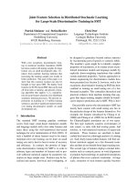
Figure 1: An example of a PST. The root node corresponds to the empty suffix, the nodes in the first level correspond to suffixes of order
one, and so forth. The string inside each node is a memorized suffix and the adjacent vector is its probability distribution over the next
symbol of the alphabet Σ ={a, b, c, d, r}. For example, the probability to observe c after the substring bara, whose largest suffixinthe
tree is ra,isP(c|bara) = P
ra
(c) = 0.4. Similarly, since suff (bacara) = ra, the probabilities P(σ|bacara) ={0.05, 0.25, 0.4, 0.25, 0.05} for
σ ∈{a, b, c, d, r},respectively.
Ron et al. introduced a learning algorithm using a construc-
tion called prediction suffix tree (PST), which preserves the
minimal subsequences (of variable lengths) that are neces-
sary for precise modeling of the given statistical source (see
Figure 1).

While the motivation of Ron et al. was to provide genera-
tive statistical modeling for a single source, the current work
uses the PST construction to address super vised discrimina-
tion tasks. Thus, our first step is to extend the original gen-
erative VMM modeling technique to handle se veral sources
simultaneously. Next, since we wish to use the resulting mul-
ticlass model to classify new (test) sequences, we are less con-
cerned with preserving source statistics. Rather, we focus on
identifying variable length dependencies, that can serve as
good discriminative features between the learned categories.
This results in a new algorithm, termed discriminative VMM
(DVMM).
Our feature selection scheme is based on maximizing
conditional mutual information (MI). More precisely, for any
subsequence s we estimate the information between the next
symbol in the sequence and each statistical source c ∈ C,
given that subsequence (or suffix) s. We use this estimate as
a new measure for pruning less discriminative features out
of the model. This yields a criterion which is very different
from the one used by the original generative VMM model. In
particular, many features may be important for good model-
ing of each source independently although they provide mi-
nor discrimination power. These features are pruned in the
DVMM, resulting in a much more compact model which still
attains high classification accuracy.
We further suggest a natural sorting of the features re-
tained in the DVMM model. This allows an examination
of the most discriminative features, often gaining useful in-
sights about the nature of the data.
1.1. Related work

The use of MI for feature selection is well known in machine
learning realm, though it is usually suggested in the context
of “static” rather than stochastic m odeling. The original idea
may be traced back to Lewis [5]. It is motivated by the fact
that when the a priori class uncertainty is given, maximizing
the MI is equivalent to the minimization of the conditional
entropy. This in turn links MI maximization and the decrease
in classification error,
1
H

P
err

+ P
err
log(C − 1) ≥ H(C|X) ≥ 2P
err
, (1)
where
H(·) =−

P(·)logP(·),
H(·|·) =−

P(·, ·)logP(·|·)
(2)
are the entropy and the conditional entropy, respectively.
Since then, a number of methods have been posed, dif-
fering essentially by their method of approximating the joint

and marginal distributions, and their direct usage of the mu-
tual information measure (cf. [8, 9, 10]). One of the diffi-
culties in applying MI based feature selection methods, is
the fact that evaluating the MI measure involves integrat-
ing over a dense set, which leads to a computational over-
load. To circumvent that, Torkkola and Campbell [11]have
recently suggested to perform feature transformation (rather
than feature selection) to a lower-dimensional space in which
the training and analysis of the data is more feasible. Their
method is designed to find a linear transformation in the
feature space that will maximize the MI between the trans-
formed data and their class labels, and the reduction in com-
putational load is achieved by the use of Renyi’s entropy
based definition of mutual information which is much more
easy to evaluate.
Out of numerous feature selection techniques found in
the literature, we would like to point out the work of Della
Pietra et al. [12] who devised a feature selection (or rather,
induction) mechanism to build n-grams of varying lengths,
and McCallum’s “U-Tree” [13], which build PSTs based on
1
The upper bound is due to Fano’s inequality (cf. [6]), and the lower
bound can be found, for example, in [7].
Discriminative Feature Selection via Multiclass Variable Memory Markov Model 95
the ability to predict the future discounted reward in the con-
text of reinforcement learning.
Another popular approach in language modeling is the
use of pruning as a mean for parameter selection from a
higher-order n-gram backoff
2

model. One successful prun-
ing criterion, suggested by Stolcke [15], minimizes the “dis-
tance” (measured by relative entropy) between the distribu-
tions embodied by the original and the pruned models. By
relating relative entropy to the relative change in training set
perplexity,
3
a simple pruning criterion is devised, which re-
moves from the model all n-grams that change perplexity by
less than a threshold. Stolcke shows [15] that in practice this
criterion yields a significant reduction in model size without
increasing classification error.
A selection criterion, similar to the one we propose here,
was suggested by Goodman and Smyth for decision tree de-
sign [7]. Their approach chooses the “best” feature at any
node in the tree, conditioned on the features previously cho-
sen, and the outcome of evaluating those features. Thus,
they suggested a top-down algorithm based on greedy se-
lection of the most informative features. Their algorithm
is equivalent to the Shannon-Fano prefix coding, and can
also be related to communication problems in noisy chan-
nels with side information. For feature selection, Goodman
and Smyth noted that with the assumption that all features
are known a priori, the decision tree design algorithm will
choose the most relevant features for the classification task,
and ignore irrelevant ones. Thus, the tree itself yields valu-
able information on the relative importance of the various
features.
A related usage of MI for stochastic modeling is the
maximal mutual information (MMI) approach for multi-

class model training. This is a discriminative training ap-
proach attributed to Bahl et al. [16], designed to directly
approximate the posterior probability distribution, in con-
trast to the indirect approach, via Bayes’ formula, of maxi-
mum likelihood (ML) training. The MMI method was ap-
plied successfully to Hidden Markov Models (HMM) train-
ing in speech applications (see, e.g., [17, 18]). However,
MMI training is significantly more expensive than ML train-
ing. Unlike ML tr aining, in this approach all models af-
fect the training of every single model through the denom-
inator. In fact this is one reason why the MMI method
is considered to be more complex. Another reason is that
there are no known easy re-estimation formulas (as in ML).
Thus we need to resort to general purpose optimization
techniques.
Our approach stems from a similar motivation but it sim-
plifies matters: we begin with a simultaneous ML training for
all classes and then select features that maximize the same ob-
2
The backoff recursive rule (cf. [14]) represents n-gram conditional
probabilities P(w
n
|w
n−1
···w
1
) using (n − 1)-gram conditional probabili-
ties multiplied by a backoff weight, α(w
n−1
···w

1
), associated with the full
history, that is, P(w
n
|w
n−1
···w
1
) = α(w
n−1
···w
1
)P(w
n
|w
n−1
···w
2
),
where α is selected such that

P(w
n
|w
n−1
···w
1
) = 1.
3
Perplexity is the average branching factor of the language model.

jective function. While we cannot claim to directly maximize
mutual information, we provide a practical approximation
which is far less computationally demanding.
2. VARIABLE MEMORY MARKOV MODELS
Consider the classification problem to a set of categories
C ={c
1
,c
2
, ,c
|C|
}. The training data consists of a set of
labeled examples for each class. Each sample is a sequence of
symbols over some alphabet Σ. A Bayesian learning frame-
work trains generative models to produce good estimates of
class conditioned probabilities, which in turn, upon receiv-
ing a new (test) sample d, are employed to yield Maximum A
Posteriori (MAP) decision rule
max
c∈C
P(c|d) ∝ max
c∈C
P(d|c)P(c),d∈ Σ
∗
. (3)
Thus, good estimates of P(d|c) are essential for accurate clas-
sification. Let d = σ
1
,σ
2

, ,σ
|d|
, σ
i
∈ Σ, and let s
i
∈ Σ
i−1
denote the subsequence of symbols preceding to σ
i
, then
P(d|c) =
|d|

i=1
P

σ
i
|σ
1
σ
2
···σ
i−1
,c

=
|d|


i=1
P

σ
i
|s
i
,c

. (4)
Denoting by suff (s
i
) the longest suffixofs
i
, we know that if
P(σ
|s
i
) = P(σ |suff(s
i
)), for every σ ∈ Σ, then predicting the
next symbol using s
i
is equivalent to a prediction using the
shorter context given by suff (s
i
). Thus, in this case it is clear
that keeping only suff (s
i
) in the model should suffice for the

prediction.
The VMM algorithm [4] aims at building a model which
will hold only a minimal set of relevant suffixes. To this end, a
suffixtree
ˆ
T is built in two steps. First, only suffixes s ∈ Σ
∗
for
which the empirical probability in the training data,
ˆ
P(s), is
nonnegligible, are kept in the model. Thus, rare suffixes are
ignored. Next, all suffixes that are not informative for pre-
dicting the next symbol are pruned out of the model. Specif-
ically, this is done by thresholding r ≡ P(σ|s)/P(σ|suff (s)).
If r ≈ 1forallσ ∈ Σ, then predicting the next symbol using
suff (s) is almost identical to using s.Insuchcasess will be
pruned out of the model.
3. MULTICLASS DISCRIMINATIVE VMM
The VMM algorithm is designed to statistically approximate
a single source. A straightforward extension to handle mul-
ticlass categorization tasks would build a separate VMM for
each class, based solely on its own data, and would classify
a new example to the model with the highest score (a one-
versus-all approach, e.g., [19]).
Motivated by a generative goal, this approach disregards
the possible (dis)similarities between the different categories.
Each model aims at best approximating its assigned source.
However, in a discriminative framework these interactions
may b e exploit to our benefit. As a simple example, assume

that for some suffix s and every symbol σ ∈ Σ,
ˆ
P(σ|s, c) =
ˆ
P(σ|s)forallc ∈ C, that is, the symbols and the categories
96 EURASIP Journal on Applied Signal Processing
Initialization and first step—tree growing:
Initialize
ˆ
T to include the empty suffix e,
ˆ
P(e) = 1.
For l = 1 L
for every s
l
∈ Σ
l
,wheres
l
= σ
1
σ
2
···σ
l
, estimate
ˆ
P(s
l
|c) =


l
i=1
ˆ
P(σ
i
|σ
1
···σ
i−1
,c)
if
ˆ
P(s
l
|c) ≥ ε
1
,forsomec ∈ C,adds
l
into
ˆ
T.
Second step—pruning:
For all s ∈
ˆ
T, estimate I
s
=

c∈C

ˆ
P(c|s)

σ∈Σ
ˆ
P(σ|s, c)log(
ˆ
P(σ|s, c)/
ˆ
P(σ|s)).
For l = L 1
define
ˆ
T
l
≡ Σ
l
∩
ˆ
T
for every s
l
∈
ˆ
T
l
,
let
ˆ
T

s
l
be the subtree spanned by s
l
define
¯
I
s
l
= max
s

∈
ˆ
T
s
l
I
s

if
¯
I
s
l
− I
suff (s
l
)
≤ ε

2
, prune s
l
.
Algorithm 1: Pseudo-code for the DVMM training algorithm.
are independent given s. Since we are only interested in the rel-
ative order of the posteriors
ˆ
P(c|s), these terms may as well be
neglected. In other words, preserving s in the model will y ield
no contribution to the classification task, since this suffixhas
no discrimination power with respect to the given categories.
We now turn to generalize and quantify this intuition. In
general, two random variables X and Y are independent if
and only if the MI between them is zero (cf. [6]). For e very
s ∈ Σ
∗
, we consider the following (local) conditional MI,
I
s
≡ I(Σ; C|s) =

c∈C
ˆ
P(c|s)

σ∈Σ
ˆ
P(σ|c,s)log
ˆ

P(σ|c,s)
ˆ
P(σ|s)
, (5)
where
ˆ
P(c|s) is estimated using Bayes’ formula,
ˆ
P(c|s) =
ˆ
P(s|c)
ˆ
P(c)/
ˆ
P(s), the prior
ˆ
P(c) can be estimated by the rel-
ative number of training examples labeled with the category
c, or from domain knowledge, and
ˆ
P(s) =

c∈C
ˆ
P(c)
ˆ
P(s|c).
If I
s
= 0, as above, s can certainly be pruned. However, we

may define a stronger pruning criterion, which consider also
the suffixofs.Specifically,ifI
s
−I
suff (s)
≤ ε
2
,whereε
2
is some
threshold, one may prune s and settle for the shorter mem-
ory suff(s). In other words, this criterion implies that suff(s)
effectively induces more dependency between Σ and C than
its extension s. Thus, preserving suff(s) in the model should
suffice for the classification task.
4
Finally, note that as in the original VMM, the pruning
criterion defined above is not monotone. Thus, it is possible
to get I
s
1
>I
s
2
<I
s
3
for s
3
= suff (s

2
) = suff (suff(s
1
)). In
this case we may be tempted to prune the “middle” suffix
s
2
along with its child, s
1
, despite the fact that I
s
1
>I
s
3
.To
avoid that we define the pruning criterion more carefully. We
denote by
ˆ
T
s
the subtree spanned by s, that is, all the nodes
in
ˆ
T
s
correspond to subsequences with the same suffix, s.We
can now calculate
¯
I

s
= max
s

∈
ˆ
T
s
I
s

, and define the pruning
criterion by
¯
I
s
− I
suff (s)
≤ ε
2
. Therefore, w e prune s (along
4
Indeed, in general, conditioning reduces entropy, and therefore in-
creases MI, but this does not say anything about the individual terms at the
MI summation which may exhibit an opposite relation (cf. [6]).
with all its descendants), only if there is no descendant of s
(including s itself) that induces more information (up to ε
2
)
between Σ and C,comparedtosuff(s), the parent of s.We

term this algorithm DVMM training (see Algorithm 1).
4. SORTING THE DISCRIMINATIVE FEATURES
The above procedure yields a rather compact discr iminative
model b etween several statistical sources. Naturally not all its
features have the same discriminative power. We denote the
information content of a feature by
I
σ|s
≡

c∈C
ˆ
P(c|s)
ˆ
P(σ|s, c)log

ˆ
P(σ|s, c)
ˆ
P(σ|s)

. (6)
Note that I
s
=

σ∈Σ
I
σ|s
,thusI

σ|s
is simply the contribution
of σ to I
s
.If
ˆ
P(σ|s, C) ≈
ˆ
P(σ|s), meaning σ and C are almost
independent given s, then I
σ|s
will be relatively small, and vice
versa.
This criter ion can be applied to sort a ll the DVMM
features. Still, it might be that I
σ
1
|s
1
= I
σ
2
|s
2
, while
ˆ
P(s
1
) 
ˆ

P(s
2
). Clearly in this case one should prefer the first feature,
{s
1
·σ
1
}, since the probability to encounter it is higher. There-
fore, we should balance between I
σ|s
and
ˆ
P(s) when sorting.
Specifically, we score each feature by
ˆ
P(s)I
σ|s
, and sort in de-
creasing order.
The pruning and sorting schemes above are based on lo-
cal conditional mutual information values. We review the
process from a global standpoint. The global conditional mu-
tual information is given by (see, e.g., [6])
I(Σ; C
|S) =

s∈Σ
∗
ˆ
P(s)I(Σ; C|s) =


s∈Σ
∗
ˆ
P(s)I
s
=

s∈Σ
∗

σ∈Σ
ˆ
P(s)I
σ|s
.
(7)
First we neglect all suffixeswitharelativelysmallprior
ˆ
P(s).
Then we prune all suffixes s for which
¯
I
s
is small with re-
spect to I
suff (s)
. Finally, we sort all remaining features by their
Discriminative Feature Selection via Multiclass Variable Memory Markov Model 97
contribution to the global conditional mutual information,

given by
ˆ
P(s)I
σ|s
. Thus, we aim for a compact model that still
strives to maximize I(Σ; C|S).
Expressing the conditional MI as the difference between
two conditional ent ropies, I(Σ; C|S) = H(C|S) − H(C|S, Σ),
we see that maximizing I(Σ; C|S) is equivalent to minimizing
H(C|Σ,S). In other words, our procedure effectively tries to
minimize the entropy, that is, the uncertainty, over the cat-
egory identity C given the new symbol Σ and the suffix S,
which in turn decreases the classification error (see (1)).
5. EXPERIMENTAL RESULTS
To test the validity of our method we performed a com-
parative analysis over several data types. In this section, we
describe the results for protein and text classification tasks.
Other applications, such as DNA sequence analysis, will be
presented elsewhere.
5.1. Experimental design
In every dataset the DVMM algorithm is compared with two
different ( although related) algorithms. A natural compar-
ison is of course with the original generative VMM model
[4]. In a recent work, Bejerano and Yona [19] s uccessfully
applied a one-versus-all approach to protein classification,
building a generative VMM for each family, in order to esti-
mate the membership probability of new protein to that fam-
ily. Specifically, it was shown that one may accurately identify
whether a protein is a member in that family or not. In our
context, we build |C| different generative models, one per

class. A new example is then classified into the most prob-
able class using these models. We will term this approach
GVMM.
We further compared our results to A. Stolcke’s perplex-
ity pruning SRILM language modeling toolkit
5
(discussed in
Section 1.1). Here, again, |C| generative models are trained
and classification is to the most probable class. Since the
SRILM toolkit is limited to 6-grams, we bounded the max-
imal depth of the PST’s (for both DVMM a nd GVMM)
to the equivalent suffix length 5. For all three models, we
neglected in the first step (of ignoring small
ˆ
P(s)) all suf-
fixes appearing less than twice in the training sequences.
In principle, these two parameters can be fine tuned for
a specific data set using standard methods, such as cross
validation.
For pruning purposes we vary the analogous local deci-
sion threshold parameter in all three methods to obtain dif-
ferent model sizes. These are ε
2
,r, and the perplexity thresh-
oldforDVMM,GVMM,andSRILM,respectively.Inorder
tocomputemodelsizeswesumthenumberofclassspecific
features (s · σ combinations) in each model.
6
Finally, there is the issue of smoothing zero probabili-
ties. Quite a few smoothing techniques exist, some widely

5
See />6
For the DVMM this will be the number of retained nodes multiplied by
|Σ||C|.
Table 1: Details of the protein super-family test.
Class Protein family name #Proteins
c
1
Fungal lignin peroxidase 29
c
2
Animal haem peroxidase 33
c
3
Plant ascorbate pe roxidase 26
c
4
Bacterial haem catalase/peroxidase 30
c
5
Secretory plant peroxidase 102
used by language modeling researchers (see [14]forasur-
vey). Most of these incorporate two basic ideas: modifying
the true counts of the n-grams to pseudo counts (which es-
timate expected rather than observed counts), and interpo-
lating higher-order with lower-order n-gram models to com-
pensate for under sampling. For SRILM we used a standard
absolute-discounting (see [14]). The GVMM uses propor-
tional smoothing (see [19]). For the DVMM we applied a
simple plus 0.5 smoothing.

7
5.2. Protein classification tests
The problem of automatically classifying proteins into bio-
logically meaningful families has become very important in
the last few years. For this data, obviously, there is no clear
definition of higher-order features. Thus, usually each pro-
tein is represented by its ordered sequence of amino acids,
resulting in a natural alphabet of all 20 different amino acids
plus 3 ambiguity symbols.
There are various approaches to the classification of pro-
teins into families, however most of these methods agree on
a wide subset of the known protein world. We have chosen
to compare our results to those of the PRINTS database [20]
as its approach resembles ours. This database is a collection
of protein family fingerprints. Each family is matched with
a fingerprint of one or more short subsequences which have
been iteratively refined using database scanning procedures
to maximize their discrimination power in a semi-automatic
procedure involving human supervision and intervention.
5.2.1 A protein super-family test
We first used a subset of five related protein families, al l
members of the Haem peroxidase super-family, taken from
the PRINTS database (see Table 1 for details). Peroxidases are
Haem-containing enzymes that use hydrogen peroxide as the
electron acceptor to catalyse a number of oxidative reactions.
We randomly chose half of the sequences as the training set
and used the remaining half as test set. We repeated this pro-
cess 10 times and averaged the results. For each iteration we
used the training set to build the (discriminative/generative)
training model(s), and then used these model(s) to classify

the test sequences. DVMM and GVMM prediction were ob-
tained using (4), where s
i
corresponds to the maximal suffix
kept in the model during training.
7
Notice that in all our exper iments the alphabet size is fairly small (below
40). Arguably, this implies that sophisticated smoothing is less needed here,
compared to large vocabularies of up to 10
5
symbols (words).
98 EURASIP Journal on Applied Signal Processing
In Figure 2a we compare the classification accuracy of
all algorithms for different model sizes (by sweeping the
pruning parameter). All algorithms achieved perfect (or near
perfect) classification using the minimal ly pruned model.
However, using more intensive pruning (and hence, smaller
models), DVMM consistently outperforms the other two al-
gorithms. This is probably due to the fact that the DVMM
is directly trying to minimize the discrimination error, while
the other two are not. Interestingly, for the GVMM the results
are not monotonic. Very small models outperform medium-
sized models. This phenomenon, apparent also in the text
example that follows, merits further investigation.
Equally interesting here is the list of best discriminating
features. In Ta ble 2 we present the top 10 features with re-
spect to all suffixesoflength4,foundbytheDVMMalgo-
rithm (using all the data for this run). Eight of them coin-
cide with the fingerprints chosen by the PRINTS database
to represent the respective classes. The other two short mo-

tifs which have no match in the PRINTS database are how-
ever good features as they appear in no other class but their
respective one. In general these can suggest improvements
for the PRINTS fingerprint, which is usually started from a
manually crafted set of subsequences. It can also draw at-
tention to conserved motifs, of possible biological impor-
tance, which a multiple alignment program (a generative
method) or a human curator may have failed to notice. Fi-
nally, notice that the first seven entries in our table share
but three different suffixes between them, where in each case
the next symbol separates between two different classes (e.g.,
R, V separate ARDS into classes 1 and 5, respectively. Nei-
ther appear in any of the other 4 classes). This allows to
highligh t polymorphisms which are family specific and thus
of special interest when considering the molecular reason-
ing behind a biological subclassification. When a polymor-
phic site is not surrounded by a rather large conserved region
which serves to guide a generative model such as an align-
ment tool or an HMM, these methods may very well fail to
recognize it.
5.2.2 A protein domain test
As a second, harder test we used another subset of five pro-
tein groups taken from the same PRINTS database [20]
(see Tab le 3 for details). However these five groups do not
share a super-family. Rather, they all share a common do-
main (a domain is an independent protein structural unit).
The distinction becomes clearer when we notice the mem-
bers of the S-crystallin group share the same domain (and
thus an evolutionary origin) with the other four groups,
and yet the domain appears to perform a different function

in them. In all other groups the glutathione S-transferase
(GST) domain participates in the detoxification of reac-
tive electrophilic compounds by catalysing their conjuga-
tion to glutathione. We specifically chose this test since a
well-established database of protein families HMMs,
8
cur-
rently considered the state-of-the-art in generative modeling
8
The Pfam database, available at />10
2
10
3
10
4
10
5
10
6
N
0.9
0.96
1.02
Acc
Protein super-family test
DVMM SRILM PST
(a)
10
2
10

3
10
4
10
5
10
6
N
0.7
0.75
0.8
0.85
0.9
0.95
1
Acc
Protein domain test
DVMM
SRILM PST
(b)
10
7
10
6
10
5
10
4
10
3

10
2
N
0.4
0.5
0.6
0.7
0.8
0.9
1
F1
Text classification test (F1)
DVMM
SRILM PST
(c)
Figure 2: Comparison of the three algorithms. (a) Accuracy ver-
sus model size for all three algorithms over the protein super-family
test. (b) Accuracy versus model size for all three algorithms over the
protein domain test. (c) Micro-averaged F1 (see text) versus model
size for all three algorithms over the text classification test.
Discriminative Feature Selection via Multiclass Variable Memory Markov Model 99
Table 2: Correlation between the top sorted features extracted by the DVMM and known motifs, for the protein super-family test. The
left column presents the top 10 features among all features with memory length 4. For example, the first feature corresponds to the suffix
s = ARDS followed by the symbol R (the characters represent different amino acids). Additionally, the category for which
ˆ
P(σ|s, c)was
maximized is indicated (categories are ordered as in Tab le 1). For the other categories,
ˆ
P(σ|s, c


) was usually close to zero, and never exceeded
0.1. Second and third columns present
ˆ
P(σ|s, c)and
ˆ
P(s|c) for the same (maximizing) category. The next column give the percentage of
occurrences for this feature in the complete set of protein sequences in this category. The last column indicate the percentage of occurrences
for this feature only in the PRINTS fingerprint of this family. For example, the feature ARDS|R is a subsequence of a motif of the first family.
It appears in this motif for 62% of the proteins assigned to it. In this table all features either came for a PRINTS motif or from elsewhere in
the protein sequences (and thus the all or nothing correspondence between the last two columns).
Feature
ˆ
P(σ|s, c)
ˆ
P(s|c) Sequence correlation Fingerprint correlation
c
1
: ARDS|R 0.65 0.0019 62% 62%
c
3
: GLLQ|L 0.64 0.0029 73% 73%
c
5
: ARDS|V 0.66 0.0009 26% 0%
c
5
: GLLQ|S 0.38 0.0006 11% 11%
c
3
: IVAL|S 0.68 0.0035 88% 88%

c
5
: GLLQ|T 0.29 0.0006 8% 8%
c
5
: IVAL|A 0.28 0.0002 4% 4%
c
4
: PWWP|A 0.59 0.0008 64% 64%
c
4
: ASAS|T 0.40 0.0005 20% 20%
c
2
: FSNL|S 0.49 0.0004 30% 0%
Table 3: Details of the protein domain test.
Class Family name #Proteins
c
1
GST—no class label 298
c
2
Scrystallin 29
c
3
Alpha class GST 40
c
4
Mue class GST 32
c

5
Pi class GST 22
of protein families, has chosen not to model these groups
separately, due to high sequence similarity between mem-
bers of the different groups. Additionally, the empirical prior
probability
ˆ
P(C) in this test was especially skewed, since we
used all GST proteins with no known subclassification as
one of the groups. This is also a known difficulty for clas-
sification schemes. The experimental setting, including the
parameter values, were exactly the same as for the prev ious
test (i.e., 10 random splits into e qually sized training and test
set, etc.).
In spite of the above-mentioned potential pitfalls, we still
found DVMM to perform surprisingly well in this test (see
Figure 2b). Using the minimally pr uned model, the DVMM
attained almost 98% accuracy. Moreover, for all obtained
model s izes, the DVMM clearly outperformed the other two
algorithms. For example, the accuracy of the DVMM while
using only ≈ 500 features was comparable to the accuracy of
the GVMM while using ≈ 400, 000 features.
This relation may be explained by the high similarity be-
tween members of all classes. Since, in particular, each class
displays a rich conserved str ucture—the GVMM concen-
trates on modeling this struc ture, disregarding the fact that
it is commonly shared by all five classes. The DVMM on the
other hand ignores all common statistical features, homing
in only on the discriminative ones, which we know to be few
in this case.

Again, in Ta ble 4 we discuss the top 10 sorted features
with respect to all suffixes of length 4, and their correlation
with known motifs.
5.3. Text classification test
Finally, we demonstrate the performance of the DVMM algo-
rithm in a standard text classification task. In this experiment
we set Σ to be the set of characters present in the documents.
Our pre-processing included lowering upper case characters
and ignoring all non-alpha-numeric characters.
Obviously, this representation ignores the special role of
the blank character as a separator between different words.
Still, in many situations (as in the above protein classifica-
tion task) the correct segmentation is unknown, leaving one
with the basic alphabet. It should be interesting to examine
text classification using the DVMM, where we take Σ to be
the set of different words that occurred in the documents.
9
There we expect the DVMM to extract the most discriminant
word phrases between the different categories. However, this
implementation (which will probably call for sophisticated
smoothing as well) is left for future research.
9
The alphabet size (and node out degree) is in general not bounded in
this case. However, previous work by Pereira et al. [21]suggestspractical
solutionstothissituation.
100 EURASIP Journal on Applied Signal Processing
Table 4: Correlation of the top sorted features extracted by the DVMM and known motifs for the protein domain test. The column headings
are the same as in Table 2 .Classc
1
was constructed from all GST domain-containing proteins not sharing any class specific, PRINTS or other

protein database, signature. Thus they do not have a PRINTS fingerprint. Testimony of the relative difficulty of this task can be found in
the fact that now only 3 of the top 10 features are unique to their class. Moreover, 6 of these features appear solely outside the PRINTS
fingerprints, giving leads to a finer analysis of the GST sequences which will be done elsewhere.
Feature
ˆ
P(σ|s, c)
ˆ
P(s|c) Sequence correlation Fingerprint correlation
c
3
: AAGV|E 0.74 0.0037 77% 52%
c
2
: AAGV|Q 0.38 0.0020 31% 0%
c
2
: YIAD|C 0.49 0.0016 34% 31%
c
5
: LDLL|L 0.43 0.0029 45% 0%
c
1
: YIAD|K 0.46 0.0003 4% —
c
3
: YFPV|F 0.42 0.0011 20% 0%
c
2
: GRAE|I 0.70 0.0043 93% 0%
c

5
: DGDL|T 0.49 0.0031 54% 50%
c
5
: YFPV|R 0.45 0.0026 45% 0%
c
5
: KEEV|V 0.51 0.0029 54% 0%
We used the standard Reuters-21578 collection.
10
In par -
ticular, we took the ModeApte split and concentrated on the
10 most frequent categories. This resulted with a training set
of 7194 documents and a test set of 2788 documents. We
note that about 9% of these documents are multi-labeled
while our implementation induces uni-labeled classification
(where each document is classified only to its most probable
class).
In gener al, we used the same parameter settings for all
algorithms as in the previous section. However, to avoid ex-
ceeding memory capacity, in the first stage of the DVMM and
GVMM algorithms we neglected all suffixes which appeared
less than 50 times in the training set. In this setting, the run
time of the DVMM (including classification) over the whole
corpus was about two minutes (using a 733 MHz PC running
Linux).
In Figure 2c we present the micro-averaged F1 results for
different model sizes for all algorithms.
11
As in the previous

tests, the DVMM results are consistently comparable or su-
perior to the other algorithms. Specifically, while using the
minimally pruned model, the micro-averaged precision and
recall of the DVMM are 95% and 87%, respectively. This
implies a break-even performance of at least 87% (proba-
bly higher). We therefore compared these results with the
break-even performance reported by Dumais et al. [23]for
10
Available at iddlew is.com/resources/testcollections/
reuters21578/.
11
The F1 measure is the harmonic average of the standard recall and pre-
cision measures: F1 = 2pr/(p + r) (see, e.g., [22]). It is easy to verify that
for a uni-labeled dataset and a uni-labeled classification scheme, the micro-
averaged precision and recall are equivalent, and hence equal to the F1 mea-
sure. Therefore, for the protein c lassification tests we simply reported the
micro-averaged precision (which we termed “accuracy”). However, since the
Reuters corpus is multi-labeled, our Recall performance was typically lower
than our Precision.
the same task. In that work the authors compared five differ-
ent classification algorithms: FindSim (a variant of Rocchio’s
method), Naive Bayes, Bayes nets, Decision Trees, and SVM.
The (weighted) averaged performance of the first four were
74.3%, 84.8%, 86.2%, and 88.6%, respectively. The DVMM
is thus superior or comparable to all these four. The only al-
gorithm which outperforms the DVMM was the SVM with
averaged performance of 92%.
We see these results as especially encouraging, as all of the
above algorithms were used with the words representation,
while the DVMM was using the low-level character repre-

sentation.
6. DISCUSSION AND FUTURE WORK
The main contribution of this work is in describing a well-
defined framework for learning variable memory Markov
models in the context of discriminative analysis.
12
The
DVMM algorithm enables to extra ct features with variable
length dependencies which are highly discriminative with re-
spect to the statistical sources at hand. These features are
kept while other, possibly numerous features common to all
classes, are shed. They may also gain us additional insights
into the nature of the given data.
The algorithm is efficient and could be applied to any
kind of data (which exhibits the Markov property), as long as
a reasonable definition of (or quantization to) a basic alpha-
bet can be derived. The method is especially appealing where
no natural definition of higher level features exists, and in
classification tasks where the different categories share a lot
of structure (which generative models will capture, in vain).
Several important directions are left for future work. On
12
For a related approach to discrimination, using competitive learning of
generative PSTs see [24].
Discriminative Feature Selection via Multiclass Variable Memory Markov Model 101
the empirical side, more extensive experiments are required.
For the protein data, a thorough analysis of the top discrim-
inating features and their possible biological function is ap-
pealing.
On the theoretical aspect, a formal analysis of the algo-

rithm is missing. It may even be possible to extend the theo-
retical results presented in [4], in the context of discrimina-
tive VMM models.
ACKNOWLEDGMENTS
Useful discussion with Y. Bilu, R. Bachrach, E. Schneidman,
and E. Shamir is greatly appreciated. The authors would also
like to thank A. Stolcke for his help in using the SRILM
toolkit.
REFERENCES
[1] H. Almuallim and T. G. Dietterich, “Learning with many ir-
relevant features,” in Proc. 9th National Conference on Arti-
ficial Intelligence (AAAI ’91), vol. 2, pp. 547–552, Anaheim,
Calif, USA, July 1991.
[2] G. F. Hughes, “On the mean accuracy of statistical pattern
recognizers,” IEEE Trans. on Information Theory, vol. 14, no.
1, pp. 55–63, 1968.
[3] E. B. Baum and D. Haussler, “What size net gives valid gen-
eralization?,” Neural Computation, vol. 1, no. 1, pp. 151–160,
1989.
[4] D. Ron, Y. Singer, and N. Tishby, “The power of amne-
sia: learning probabilistic automata with variable memory
length,” Machine Learning, vol. 25, pp. 237–262, 1997.
[5] P. M. Lewis, “The characteristic selection problem in recogni-
tion systems,” IRE Trans. on Information Theory, vol. 8, no. 2,
pp. 171–178, 1962.
[6] T.M.CoverandJ.A.Thomas,Elements of Information Theory,
John Wiley & Sons, New York, NY, USA, 1991.
[7] R. M. Goodman and P. Smyth, “Decision tree design from
communication theory stand point,” IEEE Trans. on Informa-
tion Theory, vol. 34, no. 5, pp. 979–994, 1988.

[8] R. B attiti, “Using mutual information for selecting features in
supervised neural net lear ning,” IEEE Transactions on Neural
Networks, vol. 5, no. 4, pp. 537–550, 1994.
[9] G. Barrows and J. Sciortino, “A mutual information measure
for feature selection with application to pulse classification,”
in IEEE Intern. Symposium on Time-Frequency and Time-Scale
Analysis, pp. 249–253, 1996.
[10] H. Yang and J. Moody, “Feature selection based on joint mu-
tual information,” in Proc. International ICSC Symposium
on Advances in Intelligent Data Analysis,Rochester,NY,USA,
June 1999.
[11] K. Torkkola and W. M. Campbell, “Mutual information in
learning feature transformation,” in Proc. 17th International
Conference on Machine Learning (ICML ’2000), pp. 1015–
1022, Stanford, Calif, USA, 2000.
[12] S. Della Pietra, V. Della Pietra, and J. Lafferty, “Inducing fea-
tures of random fields,” IEEE Trans. on Pattern Analysis and
Machine Intelligence, vol. 19, no. 4, pp. 380–393, 1997.
[13] A. K. McCallum, Reinforcement learning w ith select ive percep-
tion and hidden states, Ph.D. thesis, University of Rochester,
Rochester, NY, USA, 1996.
[14] S. F. Chen and J. T. Goodman, “An empirical study of smooth-
ing techniques for language modeling,” Tech. Rep. TR-10-98,
Harvard University, Mass, USA, August 1998.
[15] A. Stolcke, “Entropy-based pruning of backoff language mod-
els,” in Proc. DARPA Broadcast News Transcription and Under-
standing Workshop, pp. 270–274, Lansdowne, Va, USA, Febru-
ary 1998.
[16]L.R.Bahl,P.F.Brown,P.V.deSouza,andR.L.Mer-
cer, “Maximum mutual information estimation of hid-

den Markov model parameters for speech recognition,” in
Proc. IEEE Int. Conf. Acoustics, Speech, Signal Processing, vol. 1,
pp. 49–52, Tokyo, Japan, October 1986.
[17] Y. Normandin, R. Cardin, and R. De Mori, “High-
performance connected digit recognition using maximum
mutual information estimation,” IEEE Trans. Speech, and Au-
dio Processing, vol. 2, no. 2, pp. 299–311, 1994.
[18] P. C. Woodland and D. Povey, “Large scale discriminative
training for speech recognition,” in Proc. Int. Workshop on
Automatic Speech Recognition (ASR), pp. 7–16, Paris, France,
September 2000.
[19] G. Bejerano and G. Yona, “Variations on probabilistic suffix
trees: statistical modeling and prediction of protein families,”
Bioinformatics, vol. 17, no. 1, pp. 23–43, 2001.
[20] T. K. Attwood, M. J. Blythe, D. R. Flower, et al., “PRINTS and
PRINTS-S shed light on protein ancestry,” Nucleic Acids Res.,
vol. 30, no. 1, pp. 239–241, 2002.
[21] F. Pereira, Y. Singer, and N. Tishby, “Beyond word N-grams,”
in Natural Language Processing Using Ve ry Large Corpora,
K. Church, S. Armstrong, P. Isabelle, E. Tzoukermann, and
D. Yarowsky, E ds., pp. 95–106, Kluwer Academic, Dordrecht,
1999.
[22] Y. Yang, “A study on thresholding strategies for text catego-
rization,” in Proc. 24th Annual International ACM SIGIR Con-
ference on Research and Development in Information Retrieval,
pp. 137–145, New Orleans, La, USA, September 2001.
[23] S. Dumais, J. Platt, D. Heckerman, and M. Sahami, “Inductive
learning algorithms and representations for text categoriza-
tion,” in Proc. International Conference on Information and
Knowledge Management, pp. 148–155, Bethesda, Md, USA,

November 1998.
[24] G. Bejerano, Y. Seldin, H. Margalit, and N. Tishby, “Marko-
vian domain fingerprinting: statistical segmentation of pro-
tein sequences,” Bioinformatics, vol. 17, no. 10, pp. 927–934,
2001.
Noam Slonim received his B.S. degree in
computer science, physics, and mathemat-
ics in 1995 from the Hebrew University of
Jerusalem, Israel. He submitted his Ph.D.
thesis, entitled “The Information Bottle-
neck: Theory and Applications” at the He-
brew University in 2002. He is currently
a Research Associate with the Biophysics
Group of the Princeton University Physics
Department. The primary aim of his re-
search is the development of new, theoretically well founded meth-
ods for complex data analysis. In particular he is interested in meth-
ods that are based on information theory and statistical learning
theor y.
Gill Bejerano received his B.S. degree in mathematics, physics, and
computer science in 1997, Summa cum Laude. To date he is a Ph.D.
student at the School of Computer Science and Engineering, in
the Hebrew University. His primary research interests are compu-
tational molecular biology and bioinformatics, computational and
statistical learning theory and information theory. Gill Bejerano is
a recent recipient of a Best Paper by a Student Award, and a Best
Poster Award.
102 EURASIP Journal on Applied Signal Processing
Shai Fine received his Ph.D. degree in computer science from the
Hebrew University in 1999. Since then he has been a research mem-

ber at IBM Research Labs. His primary research interests are ma-
chine learning problems that arise in human-machine interaction
and incorporate temporal modeling, statistical inference, and dis-
criminative methods. Related applications are the modeling of text,
natural language understanding, speaker and speech recognition.
More recently he has been working on applying machine learning
techniques to problems in simulation-based functional verification
of hardware design.
Naftali Tishby is currently the Chair of
the Computer Engineering Program at the
School of Computer Science and Engineer-
ing and a member of the Interdisciplinary
Center for Neural Computation at the He-
brew University. He received his Ph.D. de-
gree in theoretical physics from the Hebrew
University in 1985 and has been a research
member of staff at MIT, Bell Labs, AT&T,
and NECI since then. His current research is
on the interface between computer science, statistical physics, and
computational biology. He introduced various methods from sta-
tistical mechanics into computational learning theory and machine
learning. More recently, he has been working on the foundation of
biological information processing and has developed novel learn-
ing algorithms based on information theory, such as the Informa-
tion Bottleneck method and Sufficient Dimensionality Reduction.