Báo cáo hóa học: " The Fusion of Distributed Microphone Arrays for Sound Localization" pdf
Bạn đang xem bản rút gọn của tài liệu. Xem và tải ngay bản đầy đủ của tài liệu tại đây (1.15 MB, 10 trang )
EURASIP Journal on Applied Signal Processing 2003:4, 338–347
c
2003 Hindawi Publishing Corporation
The Fusion of Distributed Microphone Arrays
for Sound Localization
Parham Aarabi
Department of Electrical and Computer Engineering, University of Toronto, Toronto, O ntario, Canada M5S 3G4
Email:
Received 1 November 2001 and in revised form 2 October 2002
This paper presents a general method for the integration of distributed microphone arrays for localization of a sound source. The
recently proposed sound localization technique, known as SRP-PHAT, is shown to be a special case of the more general microphone
array integration mechanism presented here. The proposed technique utilizes spatial likelihood functions (SLFs) produced by each
microphone array and integrates them using a weighted addition of the individual SLFs. This integration strategy accounts for the
different levels of access that a microphone array has to different spatial positions, resulting in an intelligent integr ation strategy
that weighs the results of reliable microphone arrays more significantly. Experimental results using 10 2-element microphone
arrays show a reduction in the sound localization error from 0.9 m to 0.08 m at a signal-to-noise ratio of 0 dB. The proposed
technique also has the advantage of being applicable to multimodal sensor networks.
Keywords and phrases: microphone arrays, sound localization, sensor integration, information fusion, sensor fusion.
1. INTRODUCTION
The localization of sound sources using microphone arrays
has been extensively explored in the past [1, 2, 3, 4, 5, 6, 7]. Its
applications include, among others, intelligent environments
and automatic teleconferencing [8, 9, 10, 11]. In all of these
applications, a single microphone array of various sizes and
geometries has been used to localize the sound sources using
a variety of techniques.
In certain environments, however, multiple microphone
arrays may be operating [9, 11, 12, 13]. Integrating the re-
sults of these ar rays might result in a more robust sound lo-
calization system than that obtained by a single array. Fur-
thermore, in large environments such as airports, multiple
arrays are required to cover the entire space of interest. In
these situations, there will be regions in which multiple ar-
rays overlap in the localization of the sound sources. In these
regions, integrating the results of the multiple arrays may
yield a more accurate localization than that obtained by the
individual arrays.
Another matter that needs to be taken into considera-
tion for large environments is the level of access of each ar-
ray to different spatial positions. It is clear that as a speaker
moves farther away from a microphone array, the array will
be less effective in the localization of the speaker due to
the attenuation of the sound waves [14]. The manner in
which the localization errors increase depends on the back-
ground signal-to-noise ratio (SNR) of the environment and
the array geometry. Hence, given the same background SNR
and geometry for two different arrays, the array closer to
the speaker will, on an average, yield more accurate loca-
tion estimates than the array that is farther away. Conse-
quently, a symmetrical combination of the results of the two
arrays may not yield the lowest error since more s ignificance
should be placed on the results of the array closer to the
speaker. Two questions arise at this point. First, how do we
estimate or even define the different levels of access that a
microphone array may have to different spatial positions?
Second, if we do have a quantitative level-of-access defini-
tion, how do we integrate the results of multiple arrays while
at the same time accounting for the different levels of ac-
cess.
In order to accommodate variations in the spatial ob-
servability of each sensor, this paper proposes the spatial ob-
servability function (SOF), which gives a quantitative indica-
tion of how well a microphone array (or a sensor in general)
perceives events at different spatial position. Also, each mi-
crophone array will have a spatial likelihood function (SLF),
which will report the likelihood of a sound source at each
spatial position based on the readings of the current micro-
phone array [8, 13, 15]. It is then shown, using simulations
and experimental results, that the SOFs and SLFs for differ-
ent microphone arrays can be combined to result in a robust
sound localization system utilizing multiple microphone ar-
rays. The proposed microphone array integration strategy is
shown to be equivalent, in the case that all arrays have equal
access, to the array integration strategies previously proposed
[7, 12].
The Fusion of Distributed Microphone Arrays for Sound Localization 339
2. BASIC SOUND LOCALIZATION
Sound localization is accomplished by using differences in
the sound signals received at different observation points
to estimate the direction and eventually the actual loca-
tion of the sound source. For example, the human ears,
acting as two different sound observation points, enable
humans to estimate the direction of arrival of the sound
source. Assuming that the sound source is modeled as a
point source, two different clues can be utilized in sound
localization. The first clue is the interaural level difference
(ILD). Emanated sound waves have a loudness that gradu-
ally decays as the observation point moves further away from
the source [6]. This decay is proportional to the square of
the distance between the observation point and the source
location.
Knowledge about the ILD at two different observation
points can be used to estimate the ratio of the distances be-
tween each observation point and the sound source location.
Knowing this ratio as well as the locations of the observation
points allows us to constrain the sound source location [6].
Another clue that can be utilized for sound localization is the
interaural time difference (ITD), more commonly referred
to as the time difference of arrival (TDOA). Assuming that
the distance between each observation point and the sound
source is different, the sound waves produced by the source
will arrive at the observation points at different times due to
the finite speed of sound.
Knowledge about the TDOA at the different observa-
tion points and the velocity of sound in air can be used to
estimate the difference in the distances of the observation
points to the sound source location. The difference in the dis-
tances constrains the sound source location to a hyperbola
in two dimensions, or a hyperboloid in three dimensions
[8].
By having several sets of observation point pairs, it be-
comes possible to use both the ILD and the TDOA re-
sults in order to accurately localize sound sources. In real-
ity, for speech localization, TDOA-based location estimates
are much more accurate and robust than ILD-based loca-
tion estimates, which are mainly effec tive for signals with
higher frequency components than signals with components
at lower frequencies [16]. As a result, most state-of-the-
art sound localization systems rely mainly on TDOA results
[1, 3, 4, 8, 17].
There are many different algorithms that attempt to es-
timate the most likely TDOA between a pair of observers
[1, 3, 18]. Usually, these algorithms have a heuristic measure
that estimates the likelihood of every possible TDOA, and se-
lects the most likely value. There are generally three classes
of TDOA estimators, including the general cross-correlation
(GCC) approach, the maximum likelihood (ML)approach,
and the phase transform (PHAT) or frequency whitening ap-
proach [3]. All these approaches attempt to filter the cross-
correlation in an optimal or suboptimal manner, and then
select the time index of the peak of the result to be the TDOA
estimate. A simple model of the signal received by two mi-
crophones is shown as [3]
x
1
(t) = h
1
(t) ∗ s(t)+n
1
(t),
x
2
(t) = h
2
(t) ∗ s(t − τ)+n
2
(t).
(1)
The two microphones receive a time-delayed version of the
source signal s(t), each through channels with possibly
different impulse responses h
1
(t)andh
2
(t), as well as a
microphone-dependent noise signal n
1
(t)andn
2
(t). The
main problem is to estimate τ, given the microphone signals
x
1
(t)andx
2
(t). Assuming X
1
(ω)andX
2
(ω) are the Fourier
transforms of x
1
(t)andx
2
(t), respectively, a common solu-
tion to this problem is the GCC shown below [3, 7],
τ = arg max
β
∞
−∞
W(ω)X
1
(ω)X
2
(ω)e
jwβ
dw, (2)
where τ is an estimate of the original source signal delay be-
tween the two microphones. The actual choice of the weigh-
ing function W(ω) has been studied at length for general
sound and speech sources, and three different choices, the
ML [3, 19], the PHAT [3, 17], and the simple cross correla-
tion [6] are shown below,
W
ML
(ω) =
X
1
(ω)
X
2
(ω)
N
1
(ω)
2
X
2
(ω)
2
+
N
2
(ω)
2
X
1
(ω)
2
,
W
PHAT
(ω) =
1
X
1
(ω) · X
2
(ω)
,
W
UCC
(ω) = 1,
(3)
where N
1
(ω)andN
2
(ω) are the estimated noise spectra for
the first and second microphones, respectively.
The ML weights require knowledge about the spectrum
of the microphone-dependent noises. The PHAT does not re-
quire this knowledge, and hence has been employed more
often due to its simplicity. The unfiltered cross correlation
(UCC) does not utilize any weighing function.
3. SPATIAL LIKELIHOOD FUNCTIONS
Often, it is beneficial not only to record the most likely TDOA
but also the likelihood of other TDOAs [1, 15]inorderto
contrast the likelihood of a speaker at different spatial posi-
tions. The method of producing an array of likelihood pa-
rameters that correspond either to the direction or to the po-
sition of the sound source can be interpreted as generating
aSLF[12, 14, 20]. Each microphone array, consisting of as
little as 2 microphones, can produce an SLF for its environ-
ment.
An SLF is essentially an approximate (or noisy) measure-
ment of the posterior likelihood P(φ(x)|X), where X is a ma-
trix of all the signal samples in a 10–20-ms time segment ob-
tained from a set of microphones and φ(x) is the event that
there is a speaker at position x. Often, the direct computation
of P(φ(x)|X) is not possible (or tractable), and as a result, a
variety of methods have been proposed to efficiently measure
e(x)
= ψ
P
φ(x)|X
, (4)
340 EURASIP Journal on Applied Signal Processing
−5 −3 −11 3 5
Spatial x-axis
0
2
4
6
8
10
Spatial y-axis
Figure 1: SLF with the dark regions corresponding to a higher l ike-
lihood and the light regions corresponding to a lower likelihood.
where ψ(t) is a monotonically nondecreasing function of t.
The reason for wanting a monotonically nondecreasing func-
tion is that we only care about the relative values (at different
spatial locations) of the posterior likelihood and hence any
monotonically nondecreasing function of it will suffice for
this comparison.
In this paper, whenever we define or refer to an SLF, it
is inherently assumed that the SLF is related to the posterior
estimate of a speaker at position x,asdefinedby(4).
The simplest SLF generation method is to use the unfil-
tered cross correlation between two microphones, as shown
in Figure 1. Assuming that τ(x) is the TDOA between the two
microphones for a sound source at position x,wecandefine
the cross-correlation-based SLF as
e(x) =
∞
−∞
X
1
(ω)X
2
(ω)e
jwτ(x)
dw. (5)
The use of the cross correlation for the posterior like-
lihood estimate merits further discussion. The cross corre-
lation is essentially an observational estimate of P(X|φ(x)),
which is related to the posterior estimate as follows:
P
φ(x)|X
=
P
X|φ(x)
P
φ(x)
P(X)
. (6)
The probability P(φ(x)) is the prior probability of a
speaker at position x, which we define as ρ
x
. When using the
cross correlation (or any other observational estimate) to es-
timate the posterior probability, we must take into account
the “masking” of different p ositions caused by ρ
x
. Note that
the P(X)termisnotafunctionofx and hence can be ne-
glected since, for a given signal matrix, it does not change the
relative value of the SLF at different positions. In cases where
all spatial positions have an equal probability of a speaker
(i.e., ρ
x
is constant over x), the masking effect is just a con-
stant scaling of the observational estimate, and only in such
a case, we do get the posterior estimate of (5).
SLF generation using the unfiltered cross correlation is
often referred to as a delay-and-sum beamformer-based en-
ergy scans or as steered response power (SRP). Using a sim-
ple or filtered cross correlation to obtain the likelihood of
different TDOAs and using them as the basis of the SLFs is
not the only method for generating SLFs. In fact, for mul-
tiple speakers, using a simple cross correlation is one of the
least accurate and least robust a pproaches [4]. Many other
methods have generally been employed in multisensor-array
SLF generation, including the multiple signal classification
(MUSIC) algorithm [21], ML algorithm [22, 23, 24], SRP-
PHAT [7], and the iterative spatial probability (ISP) algo-
rithm [1, 15]. There are also several methods developed for
wideband source localization, including [25 , 26, 27]. Most of
these can be classified as wideband extensions of the MUSIC
or ML approaches.
The works [1, 15] describe the procedure of obtaining
an SLF using TDOA distribution analysis. Basical ly, for the
ith microphone pair, the probability density function (PDF)
of the TDOA is estimated from the histogram consisting of
the peaks of cross correlations performed on multiple speech
segments. Here, it is assumed that the speech source (and
hence the TDOA) remains stationary for the duration of
time that all speech segments are recorded. Then, each spatial
position is assigned a likelihood that is proportional to the
probability of its corresponding TDOA. This SLF is scaled so
that the maximum value of the SLF is 1 and the minimum
value is 0. Higher values here correspond to a higher likeli-
hood of a speaker at those locations.
In [7], SLFs are produced (called SRP-PHATs) for micro-
phone pairs that are generated similarly to [1, 8, 15]. The dif-
ference is that, instead of using TDOA distributions, actual
filtered cross correlations (using the PHAT cross correlation
filter) are used to produce TDOA likelihoods which are then
mapped to an SLF, as shown below,
e(x)
=
k
l
∞
−∞
X
k
(ω)X
l
(ω)e
jωτ
kl
(x)
X
k
(ω)
X
l
(ω)
dω, (7)
where e(x) is the SLF, X
i
(ω) is the Fourier transform of the
signal received by the ith microphone, and τ
kl
(x) is the array
steering delay corresponding to the position x and the kth
and lth microphones.
In the noiseless situation and in the absence of reverbera-
tions, an SLF from a single microphone array wil l be a repre-
sentative of the number and the spatial locations of the sound
sources in an environment. When there is noise and/or re-
verberations, the SLF of a single microphone array will be
degraded [3, 7, 28]. As a result, in practical situations, it is
often necessary to combine the SLFs of multiple microphone
arrays in order t o result in a more representative overall SLF.
Note that in all of the work in [1, 7, 8, 15], SLFs are produced
from 2-element microphone arrays and are simply added to
produce the overall SLF which, as will be shown, is a spe-
cial case of the more robust integration mechanism proposed
here.
In this paper, we use the notation e
i
(x) for the SLF of the
ith microphone array over the environment x which can be
The Fusion of Distributed Microphone Arrays for Sound Localization 341
0 0.2 0.4 0.6 0.8 1 1.2
x-distance to source in m (y-distance fixed at 3.5 m)
0
0.05
0.1
0.15
0.2
0.25
Observability
Figure 2: Relationship between sensor p osition and its observabil-
ity.
a 2D or a 3D variable. In the case of 2-element microphone
arrays, we also use the notation e
kl
(x) for the SLF of the mi-
crophone pair formed by the kth and lth microphones, also
over the environment x.
4. SPATIAL OBSERVABILITY FUNCTIONS
Under normal circumstances, an SLF would be entirely
enough to locate all spatial objects and events. However, in
some situations, a sensor is not able to make inferences about
a specific spatial location (i.e., blocked microphone array)
due to the fact that the sensing function provides incorrect
information or no information about that position. As a re-
sult, the SOF is used as an indication of the accuracy of the
SLF. Although several different methods of defining the SOF
exist [29, 30], in this paper, the mean square difference be-
tween the SLF a nd the actual probability of an object at a
position is used as an indicator of the SOF.
The spatial observability of the ith microphone array cor-
responding to the position x can thus be expressed as
o
i
(x) = E
e
i
(x) − a(x)
2
, (8)
where o
i
(x) is the SOF, e
i
(x) is the SLF, and a(x) is the actual
probability of an object a t position x,whichcanonlytakea
value of 0 or 1. We can relate a(x)toφ(x) as follows:
a(x)
=
1, if φ(x),
0, otherwise.
(9)
The actual probability a(x) is a Bernoulli random vari-
able with par ameter ρ
x
, the prior probability of an object at
position x. This prior probability can be obtained from the
nature and geomet ry of the environment. For example, at
spatial locations where an object or a wall prevents the pres-
−4 −3 −2 −10 1 2 34
Spatial x-axis
0
1
2
3
4
5
6
7
8
Spatial y-axis
Figure 3: A directly estimated SOF for a 2-element microphone ar-
ray. The darker regions correspond to a lower SOF and the lighter
regions correspond to a higher SOF. The location of the array is de-
picted by the crosshairs.
ence of a speaker, ρ
x
will be 0 and at other “allowed” spatial
regions, ρ
x
will take on a constant positive value.
In order to analyze the effects of spatial position of the
sound source and the obser vability of the microphone array,
an experiment was conducted with a 2-element microphone
array placed at a fixed distance of 3.5 m parallel to the spatial
y-axis and a varying x-axis distance to a sound source. The
SLF values of the sensor corresponding to the source posi-
tion were used in conjunction with prior knowledge about
the status of the source (i.e., the location of the source was
known) in order to estimate the relationship between the ob-
servability of the sensor and the x-axis position of the sensor.
The results of this experiment, which are shown in Figure 2,
suggest that as the distance of the sensor to the source in-
creases, so does the observability.
In practice, the SOF can be directly measured by plac-
ing stationary sound sources at known locations in space and
comparing it with the array SLF or by modeling the environ-
ment and the microphone arrays with a presumed SOF [14].
The modeled SOFs typically are smaller and closer to the mi-
crophone array (more accurate localizations) and are larger
further away from the array (less accurate localizations) [14].
Clearly, the SOF values will also depend upon the overall
noise in the environment. More noise will increase the value
of the SOFs (higher localization errors), while less noise will
result in lower SOFs (lower localization errors). However, for
a given environment with roughly equal noise at most loca-
tions, the relative values of the SOF will remain the same,
regardless of the noise level. As a result, in practice, we of-
ten obtain a distance-to-array-dependent SOF as shown in
Figure 3.
5. INTEGRATION OF DISTRIBUTED SENSORS
We will now utilize knowledge about the SLFs and SOFs in
order to integrate our microphone arrays. The approach here
342 EURASIP Journal on Applied Signal Processing
is analogous to other sensor fusion techniques [12, 14, 20,
31].
Our goal is to find the minimum mean square error
(MMSE) estimate of a(x), which can be derived as follows.
Assuming that our estimate is
˜
a(x), we can define our
mean square error as
m(x) =
˜
a(x)
− a(x)
2
. (10)
From estimation theory [32], the estimate
˜
a
m
(x) that
minimizes the above mean square error is
˜
a
m
(x) = E
a
a(x) |e
0
(x),e
1
(x), ]. (11)
Now, if we assume that the SLF has a Gaussian distribu-
tion with mean equal to the actual object probability a(x)
[14, 20], we can rewrite the MMSE estimate as follows:
˜
a
m
(x) = 1 · P
a(x) = 1|e
0
(x),
+0· P
a(x) = 0|e
0
(x),
= P
a(x) = 1|e
0
(x),
(12)
which is exactly equal to (using the assumption that, for a
given a(x), all SLFs are independent Gaussians)
˜
a
m
(x) =
1
1+(1− ρ
x
)/ρ
x
· exp
i
1 − 2e
i
(x)/2o
i
(x)
,
(13)
where ρ
x
is the prior sound source probability at the location
x. It is used to account for known environmental facts such as
the location of walls or desks at which a speaker is less likely
to be placed. Note that although the Gaussian model for the
SLF works well in practice [14], it is not the only model or
the best model. Other models have been introduced and an-
alyzed [14, 20].
At this point, it is useful to define the discriminant func-
tion V
x
as follows:
V
x
=
i
1 − 2e
i
(x)
2o
i
(x)
, (14)
and the overall object probability function can be expressed
as
˜
a
m
(x) =
1
1+
1 − ρ
x
· exp
V
x
/ρ
x
. (15)
Hence, similar to the approach of [1, 8, 13], additive lay-
ers dependent on individual sensors can be summed to re-
sult in the overall discriminant. The discriminant is a spatial
function indicative of the likelihood of a speaker at different
spatial positions, with lower values corresponding to higher
probabilities and higher values corresponding to lower prob-
abilities. The discriminant does not take into account the
prior sound source probabilities directly and hence a relative
comparison of discriminants is only valid for positions with
equal prior probabilities.
This decomposition greatly simplifies the integration of
the results of multiple sensors. Also, the inclusion of the
spatial observabilities allows for a more accurate model of
the behavior of the sensors, thereby resulting in greater ob-
ject localization accuracy. The integration strategy proposed
here has been shown to be equivalent to a neural-network-
based SLF fusion strategy [31]. Using neural networks often
has advantages such as direct influence estimation (obtained
from the neural weights) and the existence of strategies for
training the network [33].
5.1. Application to multimedia sensory integration
The sensor integration strategy here, while focusing on mi-
crophone arrays, can be adopted to a w ide variety of sensors
including cameras and microphones. This work has been ex-
plored in [12]. Although observabilities were not used in this
work, resulting in a possible nonideal integration of the mi-
crophone arrays and cameras, the overall result was impres-
sive. An approximately 50% reduction in the sound localiza-
tion errors was obtained at all SNRs by utilizing the audiovi-
sual sound localization system compared to the stand-alone
acoustic sound localization system. Here, the acoustic sound
localization system consisted of a 3-element microphone ar-
ray and the visual object localization system consisted of a
pair of cameras.
5.2. Equivalence to SRP-PHAT
In the case when pairs of microphones are integrated with-
out taking the spatial observabilities into account using SLFs
obtained using the PHAT technique, the proposed sensor fu-
sion algorithm is equivalent to the SRP-PHAT approach.
Assuming that the SLFs are obtained using the PHAT
technique, the SLF for the kth and lth microphones can be
written as
e
kl
(x) =
∞
−∞
X
k
(ω)X
l
(ω)e
jωτ
kl
(x)
X
k
(ω)
X
l
(ω)
dω, (16)
where X
k
(ω) is the Fourier transform of the signal obtained
by the kth microphone, X
l
(ω) is the complex conjugate of the
Fourier transform of the signal obtained by the lth micro-
phone, and τ
kl
(x) is the array steering delay corresponding
to the position x and the microphones k and l.
In most applications, we care about the relative likeli-
hoods of objects at different spatial positions. Hence, it suf-
fices to only consider the discriminant function of (14)here.
Assuming that the spatial observability of all microphone
pairs for all spatial regions is equal, we obtain the following
discriminant function:
V
x
= C
1
− C
2
i
e
i
(x), (17)
where C
1
and C
2
are positive constants. Since we care only
about the relative values of the discriminant, we can reduce
(17)to
V
x
=
i
e
i
(x), (18)
The Fusion of Distributed Microphone Arrays for Sound Localization 343
Distributed network of microphone arrays
Single equivalent microphone array
Figure 4: The integration of multiple sensors into a single “super”-
sensor.
and we note that while in (17)and(18) higher values of the
discriminant were indicative of a lower likelihood of an ob-
ject, in (18) higher values of the discriminant are now indica-
tive of a higher likelihood of an object. The summation over
i is across all the microphone arrays. If we use only micro-
phone pairs and use all available microphones, then we have
V
x
=
k
l
e
kl
(x). (19)
Utilizing (16), this becomes
V
x
=
k
l
∞
−∞
X
k
(ω)X
l
(ω)e
jωτ
kl
(x)
X
k
(ω)
X
l
(ω)
dω (20)
which is exactly equal to the SRP-PHAT equation [7].
6. EFFECTIVE SLF AND SOF
After the result of multiple sensors have been integrated, it is
useful to get an estimate of the cumulative observability ob-
tained as a result of the integration. This problem is equiv-
alent to finding the SLF and SOF of a single sensor that re-
sults in the same overall object probability as that obtained
by multiple sensors, as shown in Figure 4.
This can be stated as
P
a(x) = 1|e
0
(x),o
0
(x),
= P
a(x) = 1|e(x), o(x)
,
(21)
where e(x) is the effective SLF and o(x) is the effective SOF
of the combined sensors. According to (13), this problem re-
duces to finding equivalent discriminant functions, one cor-
responding to the multiple sensors and one corresponding
to the effective single sensors. According to (14), this be-
comes (using the constraint that the effective SLF will also
be a Gaussian)
i
1 − 2e
i
(x)
2o
i
(x)
=
1 − 2e(x)
2o(x)
. (22)
Now, we let the effective SOF be the variance of the ef-
fective SLF, or in other words, we let the effective SOF be the
observability of the effective sensor. We first evaluate the vari-
ance of the effective SLF as follows:
E
e(x) − Ee(x)
2
= o(x)
2
E
i
e
i
(x) − a(x)
o
i
(x)
2
. (23)
The random process e
i
(x) − a(x) is a zero-mean Gaus-
sian random process, and the expectation of the square of a
sum of an independent set of these random processes is equal
to the sum of the expectation of the square of each of these
processes [34 ], as shown below,
E
e(x) − Ee(x)
2
= o(x)
2
i
E
e
i
(x) − a(x)
o
i
(x)
2
. (24)
This is because all the cross-variances equal zero due to
the independency of the sensors and the zero means of the
random process. Equation (24) can be simplified to produce
E
e(x) − Ee(x)
2
= o(x)
2
i
E
e
i
(x)
2
− a(x)
2
o
i
(x)
2
. (25)
Now, by setting (25) equal to the effective observability, we
obtain
o(x) =
1
i
1/o
i
(x)
2
E
e
i
(x)
2
− a(x)
2
. (26)
Finally, noting that E(e
i
(x)
2
−a(x)
2
) = o
i
(x) according to (8),
we obtain
i
1
o
i
(x)
=
1
o(x)
, (27)
and the effective SLF then becomes
e(x) =
1
2
− o(x) ·
i
1 − 2e
i
(x)
2o
i
(x)
= o(x) ·
i
e
i
(x)
o
i
(x)
. (28)
7. SIMULATED AND EXPERIMENTAL RESULTS
Simulations were performed in order to understand the re-
lationship between SNR, sound localization error, and the
number of microphone pairs used. Figure 5 illustrates the re-
sults of the simulations. The definition of noise in these sim-
ulations corresponds to the second speaker ( i.e., the interfer-
ence signal) in the simulations. Hence, SNR in this context
really corresponds to the signal-to-interference ratio (SIR).
The results illustrated in Figure 5 were obtained by sim-
ulating the presence of a sound source and a noise source
at a random location in the environment and observing the
sound signals by a pair of microphones. The microphone
pair always has an intermicrophone distance of 15 cm but
have a random location. In order to get an average over all
speaker, noise, and array locations, the simulation was re-
peated a total of 1000 times.
Figure 5 seems to suggest that accurate and robust sound
localization is not possible, because the localization error at
low SNRs does not seem to improve when more microphone
344 EURASIP Journal on Applied Signal Processing
12345678910
Number of 2-element microphone arrays
0
0.2
0.4
0.6
0.8
1
1.2
1.4
Average localization error (m)
1dBSNR
3dBSNR
5dBSNR
7dBSNR
9dBSNR
Figure 5: Relationship between SNR, simulated sound localization
accuracy, and number of binary microphone arrays without taking
spatial observabilities into consideration.
0.31 m 0.15 m
Walls
2-element
microphone arrays
Sound localization test environment
Figure 6: The location of the 10 2-element microphone arrays i n
the test environment.
arrays are added to the environment. On the other hand,
at high SNRs, extra microphone arrays do have an impact
on the localization error. It should be noted that the results
of Figure 5 correspond to an array integration mechanism
where all arrays are assumed to have the same observability
over all spatial locations. In reality, differences resulting from
the spatial orientation of the environment and the attenu-
ation of the source signals usually result in one array to be
more observable of a spatial position than another.
An experiment was conducted with 2-element micro-
phone arrays at 10 different spatial positions as shown in
Figure 6. Two uncorrelated speakers were placed at random
positions in the environment, both with approximately equal
vocal intensity that resulted in an overall SNR of 0 dB. The
two main peaks of the overall speaker probability estimate
were used as speaker location estimates, and for each trial the
average localization error in two dimensions was calculated.
The trials were repeated approximately 150 times, with the
12345678910
Number of 2-element microphone arrays
0
0.2
0.4
0.6
0.8
1
1.2
1.4
Average localization error (m)
Experimental error at 0 dB using observabilities
Experimental error at 0 dB without using observabilities
Simulated error at 0 dB without using observabilities
Figure 7: Relationship between experimental localization accuracy
(at 0 dB) and number of binary microphone arrays both with and
without taking spatial observabilities into consideration.
first 50 times used to train the observabilities of each of the
microphone arrays by using knowledge about the estimated
speaker locations and the actual speaker locations. The lo-
calization errors of the remaining 100 trials were averaged to
produce the results shown in Figure 7. The localization errors
were computed based on the two speaker location estimates
and the true location of the speakers. Also, for each trial, the
location of the two speech sources was randomly v aried in
the environment.
As shown in Figure 7, the experimental localization er-
ror approximately matches the simulated localization error
at 0 dB for the case that all microphone arrays are assumed
to equally observe the environment. The error in this case re-
mainscloseto1mevenasmoremicrophonearraysareused.
Figure 7 also shows the localization error for the case that
the observabilities obtained from the first 50 trials are used.
In this case, the addition of extra arrays significantly reduces
the localization error. When the entire set of 10 ar rays are in-
tegrated, the average localization error for the experimental
system is reduced to 8 cm.
The same experiment was conducted with the delay-
and-sum beamformer-based SLFs (SRPs with no cross-
correlation filtering) instead of the ISP-based SLF generation
method. The results are shown in Figure 8.
The localization error of the delay-and-sum beam-
former-based SLF generator is reduced by a factor of 2 when
observability is taken into account. However, the errors are
far greater than the sound localization system that uses the
ISP-based SLF generator. When all 10 microphone pairs are
taken into account, the localization error is approximately
0.5 m.
Now, we consider an example of the localization of 3
speakers, all speaking with equal vocal intensities. Figure 9
The Fusion of Distributed Microphone Arrays for Sound Localization 345
12345678910
Number of 2-element microphone arrays
0.4
0.5
0.6
0.7
0.8
0.9
1
1.1
1.2
1.3
1.4
Average localization error (m)
Delay-and-sum sound localization without observabilities
Delay-and-sum sound localization using observabilities
Delay-and-sum sound localization using all 20 microphone
as single array
Figure 8: Relationship between experimental localization accuracy
(at 0 dB) using a delay-and-sum beamformer-based SLFs and num-
ber of binary microphone arrays both with and without taking spa-
tial observabilities into consideration.
0
2
4
6
8
Spatial y-axis
4
2
0
−2
−4
Spatial x-axis
0
0.2
0.4
0.6
0.8
1
Sound source likelihood
Figure 9: The location of 3 speakers in the environment.
illustrates the location of the speakers in a two-dimensional
environment. Note that the axis labels of Figures 9, 10,and
11 correspond to 0.31-m steps.
The ISP-based SLF generator, without taking the observ-
ability of each microphone pair into account, produces the
overall SLF shown in Figure 10 .
In Figure 10,itisdifficult to determine the true position
of the speakers. There is also a third peak that does not corre-
spond to any speaker. Using the same sound signals, an SLF
was produced and shown in Figure 11, this time with taking
observabilities into account.
This time, the location of the speakers can be clearly de-
termined. Each of the three peaks correspond to the correct
location of their corresponding speakers.
0
2
4
6
8
Spatial y-axis
4
2
0
−2
−4
Spatial x-axis
0
1
2
3
4
5
Sound source likelihood
Figure 10: Localization of 3 speakers without using observabilities.
0
2
4
6
8
Spatial y-axis
4
2
0
−2
−4
Spatial x-axis
0
0.1
0.2
0.3
0.4
0.5
0.6
Sound source likelihood
Figure 11: Localization of 3 speakers with observabilities.
For the experiments in Figures 10 and 11, the prior prob-
ability ρ
x
for all spatial p ositions was assumed to be a con-
stant of 0.3. Furthermore, the SOFs were obtained by experi-
mentally evaluating the SOF function of (8)atseveraldiffer-
ent points (for each microphone pair) and then interpolating
the results to obtain an SOF for the entire space. An example
of this SOF generation mechanism is the SOF of Figure 3.
The large difference between the results of Figures 10
and 11 merits further discussion. Basically, the main rea-
son for the improvement in Figure 11 is that for locations
that are farther away from a microphone pair, the estimates
made by that pair are weighted less significantly than micro-
phone pairs that are closer. On the other hand, in Figure 10,
the results of all microphone pairs are combined with equal
weights. As a result, even if, for every location, there are a
few microphone pairs with correct estimates, the integration
with the noisy estimates of the other microphone pairs taints
the resulting integrated estimate.
8. CONCLUSIONS
This pap er introduced the concept of multisensor object lo-
calization using different sensor observabilities in order to
346 EURASIP Journal on Applied Signal Processing
account for different levels of access to each spatial position.
This definition led to the derivation of the minimum mean
square error object localization estimates that corresponded
to the probability of a speaker at a spatial location given the
results of all available sensors. Experimental results using this
approach indicate that the average localization error is re-
duced to 8 cm in a prototype environment with 10 2-element
microphone arrays at 0 dB. With prior approaches, the local-
ization error using the exact same network is approximately
0.95 m at 0 dB.
The reason that the proposed approach outperforms its
previous counterparts is that, by taking into account which
microphone array has better access to each speaker, the effec-
tive SNR is increased. Hence, the behaviour and per formance
of the proposed approach at 0 dB is comparable to that of
prior approaches at SNRs greater than 7–10 dB.
Apart from improved performance, the proposed algo-
rithm for the integration of distributed microphone arrays
has the advantage of requiring less bandwidth and less com-
putational resources. Less bandwidth is required since each
array only reports its SLF, which usually involves far less in-
formation than transmitting multiple channels of audio sig-
nals. Less computational resources are required since com-
puting an SLF for a single array and then combining the re-
sults of multiple microphone arrays by weighted SLF addi-
tion (as proposed in this paper) is computationally simpler
than producing a single SLF directly from the audio signals
ofallarrays[14].
One drawback of the proposed technique is the measure-
ment of the SOFs for the arrays. A fruitful direction of future
work would be to model the SOF instead of experimentally
measuring it, which is a very tedious process. Another area of
potential future work is a better model for the speakers in the
environment. The proposed model, which assumes that the
actual speaker probability is independent of different spatial
positions, could be made more realistic by accounting for the
spatial dependencies that often exist in practice.
ACKNOWLEDGMENT
Some of the simulation and experimental results presented
here have been presented in a less developed manner in [20,
31].
REFERENCES
[1] P. Aarabi and S. Zaky, “Iterative spatial probability based
sound localization,” in Proc. 4th World Multi-Conference on
Circuits, Systems, Computers, and Communications,Athens,
Greece, July 2000.
[2] P. Aarabi, “The application of spatial likelihood functions to
multi-camera object localization,” in Proc. Sensor Fusion: Ar-
chitectures, Algorithms, and Applications V, vol. 4385 of SPIE
Proceedings, pp. 255–265, Orlando, Fla, USA, April 2001.
[3] M. S. Brandstein and H. Silverman, “A robust method for
speech signal time-delay estimation in reverberant rooms,” in
Proc.IEEEInt.Conf.Acoustics,Speech,SignalProcessing,pp.
375–378, Munich, Germany, April 1997.
[4] M. S. Brandstein, A framework for speech source localization us-
ing sensor arrays, Ph.D. thesis, Brown University, Providence,
RI, USA, 1995.
[5] J. Flanagan, J. Johnston, R. Zahn, and G. Elko, “Computer-
steered microphone arrays for sound transduction in large
rooms,” Journal of the Acoustical Society of America, vol. 78,
pp. 1508–1518, November 1985.
[6] K. Guentchev and J. Weng, “Learning-based three dimen-
sional sound localization using a compact non-coplanar array
of microphones,” in Proc. AAAI Spring Symposium on Intelli-
gent Environments, Stanford, Calif, USA, March 1998.
[7] J. DiBiase, H. Silverman, and M. S. Brandstein, “Robust lo-
calization in reverberant rooms,” in Microphone Arrays: Sig-
nal Processing Techniques and Applications, M. S. Brandstein
and D. B. Ward, Eds., pp. 131–154, Springer Verlag, New York,
USA, September 2001.
[8] P. Aarabi, “Multi-sense artificial awareness,” M.A.Sc. thesis,
Department of Electrical and Computer Engineering, Univer-
sity of Toronto, Toronto, Ontario, Canada, 1998.
[9] M. Coen, “Design principles for intelligent environments,”
in Proc. 15th National Conference on Artificial Intelligence,pp.
547–554, Madison, Wis, USA, July 1998.
[10] R. A. Brooks, M. Coen, D. Dang, e t al., “The intelligent room
project,” in Proc. 2nd International Conference on Cognitive
Technology, Aizu, Japan, August 1997.
[11] A. Pentland, “Smart rooms,” Scientific American, vol. 274, no.
4, pp. 68–76, 1996.
[12] P. Aarabi and S. Zaky, “Robust sound localization using multi-
source audiovisual information fusion,” Information Fusion,
vol. 3, no. 2, pp. 209–223, 2001.
[13] P. Aarabi and S. Zaky, “Integrated vision and sound local-
ization,” in Proc. 3rd International Conference on Information
Fusion, Paris, France, July 2000.
[14] P. Aarabi, The integration and localization of distributed sensor
arrays, Ph.D. thesis, Stanford University, Stanford, Calif, USA,
2001.
[15] P. Aarabi, “Robust multi-source sound localization using tem-
poral power fusion,” in Proc. Sensor Fusion: Architectures, Al-
gorithms, and Applications V, vol. 4385 of SPIE Proceedings,
Orlando, Fla, USA, April 2001.
[16] F. L. Wightman and D. Kistler, “The dominant role of low-
frequency interaural time differences in sound localization,”
Journal of the Acoustical Society of America,vol.91,no.3,pp.
1648–1661, 1992.
[17] D. Rabinkin, R. J. Ranomeron, A. Dahl, J. French, J. L. Flana-
gan, and M. H. Bianchi, “A DSP implementation of source
location using microphone arrays,” in Proc. 131st Meeting of
the Acoustical Society of America, Indianapolis, Ind, USA, May
1996.
[18] M. S. Brandstein, J. Adcock, and H. Silverman, “A practical
time-delay estimator for localizing speech sources with a mi-
crophone array,” Computer Speech & Language, vol. 9, no. 2,
pp. 153–169, 1995.
[19] C. H. Knapp and G. Carter, “The generalized correlation
method for estimation of time delay,” IEEE Trans. Acoustics,
Speech, and Signal Processing, vol. 24, no. 4, pp. 320–327, 1976.
[20] P. Aarabi, “The integration of distributed microphone arrays,”
in Proc. 4th International Conference on Information Fusion,
Montreal, Canada, July 2001.
[21] R. O. Schmidt, “Multiple emitter location and signal parame-
ter estimation,” IEEE Transactions on Antennas and Propaga-
tion, vol. 34, no. 3, pp. 276–280, 1986.
[22] H. Watanabe, M. Suzuki, N. Nagai, and N. Miki, “A method
for maximum likelihood bearing estimation without nonlin-
ear maximization,” Transactions of the Institute of Electronics,
Information and Communication Engineers A, vol. J72A, no. 8,
pp. 303–308, 1989.
The Fusion of Distributed Microphone Arrays for Sound Localization 347
[23] H. Watanabe, M. Suzuki, N. Nagai, and N. Miki, “Maximum
likelihood bearing estimation by quasi-Newton method us-
ing a uniform linear array,” in Proc. IEEE Int. Conf. Acoustics,
Speech, Signal Processing, pp. 3325–3328, Toronto, Ontario,
Canada, April 1991.
[24] I. Ziskind and M. Wax, “Maximum likelihood localiza-
tion of multiple sources by alternating projection,” IEEE
Trans. Acoustics, Speech, and Signal Processing, vol. 36, no. 10,
pp. 1553–1560, 1988.
[25] H. Wang and M. Kaveh, “Coherent signal-subspace process-
ing for the detection and estimation of angles of arrival of
multiple wide-band sources,” IEEE Trans. Acoustics, Speech,
and Signal Processing, vol. 33, no. 4, pp. 823–831, 1985.
[26] S. Valaee and P. Kabal, “Wide-band array processing using
a two-sided correlation transformation,” IEEE Trans. Signal
Processing, vol. 43, no. 1, pp. 160–172, 1995.
[27] B. Friedlander and A. J. Weiss, “Direction finding for wide-
band signals using an interpolated array,” IEEE Trans. Signal
Processing, vol. 41, no. 4, pp. 1618–1634, 1993.
[28] P. Aarabi and A. Mahdavi, “The relation between speech
segment selectivity and time-delay estimation accuracy,” in
Proc. IEEE Int. Conf. Acoustics, Speech, Signal Processing,Or-
lando, Fla, USA, May 2002.
[29] S. S. Iyengar and D. Thomas, “A distributed sensor network
structure with fault tolerant facilities,” in Intelligent Control
and Adaptive Systems, vol. 1196 of SPIE Proceedings, Philadel-
phia, Pa, USA, November 1989.
[30] R. R. Brooks and S. S. Iyengar, Multi-Sensor Fusion: Funda-
mentals and Applications with Software, Prentice Hall, Upper
Saddle River, NJ, USA, 1998.
[31] P. Aarabi, “The equivalence of Bayesian multi-sensor infor-
mation fusion and neural networks,” in Proc. Sensor Fusion:
Architectures, Algorithms, and Applications V, vol. 4385 of SPIE
Proceedings, Orlando, Fla, USA, April 2001.
[32] A. Leon-Garcia, Probability and Random Processes for Electri-
cal Engineering, Addison-Wesley, Reading, Mass, USA, 2nd
edition, 1994.
[33] B. Widrow and S. D. Stearns, Adaptive Signal Processing,
Prentice-Hall, Englewood Cliffs, NJ, USA, 1985.
[34] A. Papoulis, Probability, Random Variables and Stochastic Pro-
cesses, McGraw-Hill, New York, NY, USA, 2nd edition, 1984.
Parham Aarabi is a Canada Research Chair
in Multi-Sensor Information Systems, an
Assistant Professor in the Edward S. Rogers
Sr. Department of Electrical and Computer
Engineering at the University of Toronto,
and the Founder and Director of the Artifi-
cial Perception Laboratory. Professor Aarabi
received his B.A.S. degree in engineer-
ing science (electrical option) in 1998, his
M.A.S. degree in elect rical and computer
engineering in 1999, both from the University of Toronto, and his
Ph.D. degree in electrical engineering from Stanford University. In
November 2002, he was selected as the Best Computer Engineering
Professor of the 2002 fall session. Prior to joining the University
of Toronto in June 2001, Professor Aarabi was a Coinstructor at
Stanford University as well as a Consultant to various silicon valley
companies. His current research interests include sound localiza-
tion, microphone arrays, speech enhancement, audiovisual signal
processing, human-computer interactions, and VLSI implementa-
tion of speech processing applications.