Báo cáo hóa học: " Acoustic Source Localization and Beamforming: Theory and Practice" ppt
Bạn đang xem bản rút gọn của tài liệu. Xem và tải ngay bản đầy đủ của tài liệu tại đây (680.63 KB, 12 trang )
EURASIP Journal on Applied Signal Processing 2003:4, 359–370
c
2003 Hindawi Publishing Corporation
Acoustic Source Localization and Beamforming:
Theory and Practice
Joe C. Chen
Electrical Engineering Department, University of California, Los Angeles (UCLA), Los Angeles, CA 90095-1594, USA
Email:
Kung Yao
Electrical Engineering Department, University of California, Los Angeles (UCLA), Los Angeles, CA 90095-1594, USA
Email:
Ralph E. Hudson
Electrical Engineering Department, University of California, Los Angeles (UCLA), Los Angeles, CA 90095-1594, USA
Email:
Received 17 February 2002 and in revised form 21 September 2002
We consider the theoretical and practical aspects of locating acoustic sources using an array of microphones. A maximum-
likelihood (ML) direct localization is obtained when the sound source is near the array, while in the far-field case, we demon-
strate the localization via the cross bearing from several widely separated arrays. In the case of multiple sources, an alternating
projection procedure is applied to determine the ML estimate of the DOAs from the observed data. The ML estimator is shown
to be effective in locating sound sources of various types, for example, vehicle, music, and even white noise. From the theoretical
Cram
´
er-Rao bound analysis, we find that better source location estimates can be obtained for high-frequency signals than low-
frequency signals. In addition, large range estimation error results when the source signal is unknown, but such unknown parame-
ter does not have much impact on angle estimation. Much experimentally measured acoustic data was used to verify the proposed
algorithms.
Keywords and phrases: source localization, ML estimation, Cram
´
er-Rao bound, beamforming.
1. INTRODUCTION
Acoustic source localization has been an active research area
for many years. Applications include unattended ground sen-
sor (UGS) network for military surveillance, reconnaissance,
or around the perimeter of a plant for intrusion detection
[1]. Many var i ations of algorithms using a microphone array
for source localization in the near field as well as direction-of-
arrival (DOA) estimation in the far field have been proposed
[2]. Many of these techniques involve a relative time-delay-
estimation step that is followed by a least squares (LS) fit to
the source DOA, or in the near-field case, an LS fit to the
source location [3, 4, 5, 6, 7].
In our previous paper [8], we derived the “optimal”
parametric maximum likelihood (ML) solution to locate
acoustic sources in the near field and provided computer
simulations to show its superiority in performance over
other methods. This paper is an extension of [8], where
both the far- and the near-field cases are considered, and the
theoretical analysis is provided by the Cram
´
er-Rao bound
(CRB), which is useful for both performance comparison
and basic understanding purp oses. In addition, several ex-
periments have been conducted to verify the usefulness of
the proposed algorithm. These experiments include both in-
door and outdoor scenarios with half a dozen microphones
to locate one or two acoustic sources (sound generated by
computer speaker(s)).
One major advantage that the proposed ML approach
has is that it avoids the intermediate relative time-delay esti-
mation. This is made possible by transforming the wideband
data to the frequency domain, where the signal spectrum
can be represented by the narrowband model for each fre-
quency bin. This allows a direct optimization for the source
location(s) under the assumption of Gaussian noise instead
of the two-step optimization that involves the relative time-
delay estimation. The difficulty in obtaining relative time de-
lays in the case of multiple sources is well known, and by
avoiding this step, the proposed approach can then estimate
multiple s ource locations. However, in practice, when we ap-
ply the discrete Fourier transform (DFT), several artifacts
360 EURASIP Journal on Applied Signal Processing
can result due to the finite length of data frame (see Section
2.1.1). As a result, there does not exist an exact ML solution
for data of finite length. Instead, we ignore these finite effects
and derive the solution which we refer to as the approximated
ML (AML) solution. Note that a similar solution has been
derived independently in [9] for the far-field case.
In practice, the number of sources may be determined
independent of or together with the localization algorithm,
but here we assume that it is known for the purpose of
this paper. For the single-source case, we have shown that
the AML formulation is equivalent to maximizing the sum
of the weighted cross-correlation functions between time-
shifted sensor data in [8]. The optimization using all sensor
pairs mitigates the ambiguity problem that often arises in the
relative time-delay estimation between two widely separated
sensors for the two-step LS methods. In the case of multi-
ple sources, we apply an efficient alternating projection (AP)
procedure, which avoids the multidimensional search by se-
quentially estimating the location of one source while fixing
the estimates of other source locations from the previous it-
eration. In this paper, we demonstrate the localization results
using the AML method to the measured data, both in the
near-field and far-field cases, and for various types of sound
sources, for example, vehicle, music, and even white noise.
The AML approach is shown to outperform the LS-type al-
gorithms in the single-source case, and by applying AP, the
proposed algorithm is able to locate two sound sources from
the observed data.
The paper is organized as follows. In Section 2, the the-
oretical performances of DOA estimation and source local-
ization with the CRB analysis are given. Then, we derive the
AML solution for DOA estimation and source localization
in Section 3.InSection 4, simulation examples and experi-
mental results are given to demonstrate the usefulness of the
proposed method. Finally, we give our conclusions.
2. THEORETICAL PERFORMANCE AND ANALYSIS
In this section, the theoretical per formances of DOA estima-
tion for the far-field case and of source localization for the
near-field case are analyzed. First, we define the signal mod-
els for the far- and near-field cases. Then, the CRBs are de-
rived and analyzed. The CRB is most often used as a theo-
retical lower bound for any unbiased estimator [10]. Most
of the derivations of the CRB for wideband source localiza-
tion found in the literature are in terms of relative time-delay
estimation error. In the following, we derive a more general
CRB directly from the signal model. By developing a theoret-
ical lower bound in terms of signal characteristics and arr ay
geometry, we not only bypass the involvement of the inter-
mediate time-delay estimator but also offer useful insights to
the physical properties of the problem.
The DOA and source localization variances both depend
on two separate parts, one that only depends on the sig-
nal and another that only depends on the array geometry.
This suggests separate performance dependence on the sig-
nal and the geometry. Thus, for any given signal, the CRB
can provide the theoretical performance of a particular ge-
(x
5
,y
5
)
(x
4
,y
4
)
(x
3
,y
3
)
(x
c
,y
c
)
(x
2
,y
2
)
(x
1
,y
1
)
φ
1
φ
(2)
s
φ
(1)
s
Figure 1: Far-field example with randomly distributed sensors.
ometry and helps the design of an array configuration for a
particular scenario of interest. The signal dependence part
shows that theoretically the DOA and source location root
mean squares (RMS) error are linearly proportional to the
noise level and the speed of propagation, and inversely pro-
portional to the source spectrum and frequency. Thus, better
DOA and source location estimates can be obtained for high-
frequency signals than low-frequency signals. In fur ther sen-
sitivity analysis, large range estimation error is found when
the source signal is unknown, but such unknown parameter
does not affect the angle estimation.
The CRB analysis also shows that the uniformly spaced
circular array provides an attractive geometry for good over-
all performance. When a circular array is used, the DOA vari-
ance bound is independent of the source direction, and it
also does not degrade when the speed of propagation is un-
known. An effective beamwidth for DOA estimation can also
be given by the CRB. The beamwidth provides a measure of
how dense the angles should be sampled for the AML metric
evaluation, thus prevents unneeded iterations using numeri-
cal techniques.
Throughout this paper, we denote superscript T as the
transpose, H as the complex conjugate transpose, and ∗ as
the complex conjugate operation.
2.1. Signal model of the far- and near-field cases
2.1.1 The far-field case
When the source is in the far-field of the arr ay, the wave front
is assumed to be planar and only the angle information can
be estimated. In this case, we use the array centroid as the
reference point and define a signal model based on the rela-
tive time delays from this position. For simplicity, we assume
a randomly distributed planar (2D) arr ay of R sensors, each
at position r
p
= [x
p
,y
p
]
T
, as depicted in Figure 1.Thecen-
troid position is given by r
c
= (1/R)
R
p=1
r
p
= [x
c
,y
c
]
T
.The
sensors are assumed to be omnidirectional and have iden-
tical responses. On the same plane as the array, we assume
that there are M sources (M<R), each at an angle φ
(m)
s
Acoustic Source Localization and Beamforming: Theory and Practice 361
from the array, for m = 1, ,M. The angle convention is
such that nor th is 0 degree and east is 90 degrees. The relative
time delay of the mth source is given by t
(m)
cp
= t
(m)
c
− t
(m)
p
=
[(x
c
− x
p
)sinφ
(m)
s
+(y
c
− y
p
)cosφ
(m)
s
]/v,wheret
(m)
c
and t
(m)
p
are the absolute time delays from the mth source to the cen-
troid and the pth sensor, respectively, and v is the speed of
propagation in length unit per sample. The data collected by
the pth sensor at time n can be given by
x
p
(n) =
M
m=1
s
(m)
c
n − t
(m)
cp
+ w
p
(n), (1)
for n = 0, ,L− 1, p = 1, ,R,andm = 1, ,M,where
s
(m)
c
is the source signal arriving at the array centroid posi-
tion, t
(m)
cp
is allowed to be any real-valued number, and w
p
is
the zero-mean white Gaussian noise with variance σ
2
.
For the ease of derivation and analysis, the wideband sig-
nal model should be given in the frequency domain, where
a narrowband model can be given for each frequency bin. A
block of L samples in each sensor data can be transformed to
the frequency domain by a DFT of length N.Itiswellknown
that the DFT creates a circular time shift when applying a lin-
ear phase shift in the frequency domain. However, the time
delay in the array data corresponds to a linear time shift, thus
creating a mismatch in the signal model, which we refer to as
an edge effect. When N = L,severeedgeeffect results for
small L, but it becomes a good approximation for large L.We
can apply zero padding for small L to remove such edge ef-
fect, that is, N ≥ L + τ,whereτ is the maximum relative time
delay among all sensor pairs. However, the zero padding re-
moves the orthogonality of the noise component across fre-
quency. In practice, the size of L is limited due to the nonsta-
tionarity of the source location. In the following, we assume
that either L is large enough or the noise is almost uncorre-
lated across frequency. Note that the CRB derived based on
this frequency-domain model is idealistic and does not take
thisedgeeffect into a ccount.
In the frequency domain, the array signal model is given
by
X(k) = D(k)S
c
(k)+η(k), (2)
for k = 0, ,N − 1, where the array data spectrum is
given by X(k) = [X
1
(k), ,X
R
(k)]
T
, the steering matrix
is given by D(k) = [d
(1)
(k), ,d
(M)
(k)], the steering vec-
tor is given by d
(m)
(k) = [d
(m)
1
(k), ,d
(m)
R
(k)]
T
, d
(m)
p
(k) =
e
− j2πkt
(m)
cp
/N
, and the source spectrum is given by S
c
(k) =
[S
(1)
c
(k), ,S
(M)
c
(k)]
T
. The noise spectrum vector η(k)is
zero-mean complex white Gaussian, distributed with vari-
ance Lσ
2
. Note that, due to the transformation of the fre-
quency domain, η(k) asymptotically approaches a Gaussian
distribution by the central limit theorem even if the ac-
tual time-domain noise has an arbitrary i.i.d. distribution
(with bounded variance) other than Gaussian. This asymp-
totic property in the frequency domain provides a more reli-
able noise model than the time-domain model in some prac-
tical cases. For convenience of notation, we define S(k) =
D(k)S
c
(k). By stacking up the N/2 positive frequency bins
(zero frequency bin is not important and the negative fre-
quency bins are merely mirror images) of the signal model
in (2) into a single column, we can rewrite the sensor data
into an NR/2 × 1 space-temporal frequency vector as X =
G(Θ)+ξ,whereG(Θ) = [S(1)
T
, ,S(N/2)
T
]
T
,andR
ξ
=
E[ξξ
H
] = Lσ
2
I
NR/2
.
2.1.2 The near-field case
In the near-field case, the range infor mation can also be es-
timated in addition to the DOA. Denote r
s
m
as the location
of the mth source, and in this case we use this as the refer-
ence point instead of the array centroid. Since we consider
the near-field sources, the signal strength at each sensor can
be different due to nonuniform spatial loss in the near-field
geometry. The sensors are again assumed to be omnidirec-
tional and have identical responses. In this case, the data col-
lected by the pth sensor at time n can be given by
x
p
(n) =
M
m=1
a
(m)
p
s
(m)
0
n − t
(m)
p
+ w
p
(n), (3)
for n = 0, ,L− 1, p = 1, ,R,andm = 1, ,M,where
a
(m)
p
is the signal-gain level of the mth source at the pth sen-
sor (assumed to be constant within the block of data), s
(m)
0
is the source signal, and t
(m)
p
is allowed to be any real-valued
number. The time delay is defined by t
(m)
p
=r
s
m
−r
p
/v,and
the relative time delay between the pth and the qth sensors is
defined by t
(m)
pq
= t
(m)
p
− t
(m)
q
= (r
s
m
− r
p
−r
s
m
− r
q
)/v.
With the same edge-effect problem mentioned above, the
frequency-domain model for the near-field case is given by
X(k) = D(k)S
0
(k)+η(k), (4)
for k = 0, ,N − 1, where each element of the steering vec-
tor now becomes d
(m)
p
(k) = a
(m)
p
e
− j2πkt
(m)
p
/N
, and the source
spectrum is given by S
0
(k) = [S
(1)
0
(k), ,S
(M)
0
(k)]
T
.
2.2. Cram
´
er-Rao bound for DOA estimation
In the following CRB derivation, we consider the single-
source case (M
= 1) under three conditions: known
signal and known speed of propagation, known signal but
unknown speed of propagation, and known speed of prop-
agation but unknown signal. The comparison of the three
conditions provides a sensitivity analysis of different param-
eters. Only the single-source case is considered since valuable
analysis can be obtained using a single source while the ana-
lytic expression of the multiple-sources case becomes much
more complicated. The far-field frequency-domain signal
model for the single-source case is given by
X(k)
= S
c
(k)d(k)+η(k), (5)
for k
= 0, ,N − 1, where d(k) = [d
1
(k), ,d
R
(k)]
T
,
d
p
(k) = e
− j2πkt
cp
/N
,andS
c
(k) is the source spectrum of this
source.
362 EURASIP Journal on Applied Signal Processing
After considering all the positive frequency bins, we can
construct the Fisher information matrix [10]by
F = 2Re
H
H
R
−1
ξ
H
=
2/Lσ
2
Re
H
H
H
, (6)
where H = ∂G/∂φ
s
for the case of known signal and
known speed of propagation. In this case, the Fisher in-
formation matrix is indeed a scalar F
φ
s
= ζα,whereζ =
(2/Lσ
2
v
2
)
N/2
k=1
(2πk|S
c
(k)|/N)
2
is the scale factor that is pro-
portional to the total power in the derivative of the source
signal, and α =
R
p=1
b
2
p
is the geometry factor that depends
on the array and the source direction, where
b
p
=
x
c
− x
p
cos φ
s
−
y
c
− y
p
sin φ
s
. (7)
Hence, for any arbitrary array, the RMS error bound for DOA
estimation is given by σ
φ
s
≥ 1/
ζα. The geometry factor α
provides a measure of geometric relations between the source
and the sensor array. Poor array geometry may lead to a small
α, which results in large estimation variance. It is clear from
the scale factor ζ that the performance does not solely de-
pend on the SNR but also the signal bandwidth and spectral
density. Thus, source localization performance is better for
signals with more energy in the high frequencies.
In the case of unknown source signal, the matrix
H = [∂G/∂φ
s
,∂G/∂|S
c
|
T
,∂G/∂Φ
T
c
], where S
c
= [S
c
(1),
,S
c
(N/2)]
T
,and|S
c
| and Φ
c
are the magnitude and phase
part of S
c
, respectively. The resulting bound after applying
the well-known block matrix inversion lemma (see [11,Ap-
pendix]) on F
φ
s
,S
c
is given by σ
φ
s
≥ 1/
ζ(α − z
S
c
), where
z
S
c
= (1/R)[
R
p=1
b
p
]
2
is the penalty term due to the un-
known source signal. It is known that the DOA perfor-
mance does not degrade when the source signal is un-
known; thus, we can show that z
S
c
is indeed zero, that is,
R
p=1
b
p
= cos φ
s
R
p=1
(x
c
− x
p
) − sin φ
s
R
p=1
(y
c
− y
p
) = 0
since
R
p=1
(x
c
−x
p
) = Rx
c
−
R
p=1
x
p
= 0and
R
p=1
(y
c
−y
p
) =
0. Note that the above analysis is valid for any arbitrary ar-
ray. When the speed of propagation is unknown, the ma-
trix H = [∂G/∂φ
s
,∂G/∂v], and the resulting bound after
applying the matrix inversion lemma on F
φ
s
,v
is given by
σ
φ
s
≥ 1/
ζ(α − z
v
), where z
v
= (1/
R
p=1
t
2
cp
)[
R
p=1
b
p
t
cp
]
2
is
the penalty term due to the unknown speed of propagation.
This penalty term is not necessarily zero for any arbitrary ar-
ray, but it becomes zero for a uniformly spaced circular array.
2.2.1 The circular-array case
In the following, we show the CRB for a uniformly spaced
circular array. Not only a simple analytic form can be given
but also the optimal geometry for DOA estimation. The vari-
ance of the DOA estimation is independent of the source di-
rection, and also does not degrade when the speed of propa-
gation is unknown. Without a loss of generality, we pick the
array centroid as the origin, that is, r
c
= [0, 0]
T
. The location
of the pth sensor is given by r
p
= [ρ sin φ
p
,ρcos φ
p
]
T
,where
ρ is the radius of the circular array, φ
p
= 2πp/R+ φ
0
is the
angle of the pth sensor with respect to north, and φ
0
is the an-
gle that defines the orientation of the array. Then, α = ρ
2
R/2.
The DOA variance bound is given by σ
2
φ
s
(circular array) ≥
2/ζρ
2
R, which is independent of the source direction. It is
useful to define the following terms for a better interpreta-
tion of the CRB. Define the normalized root weighted mean
squared (nrwms) source frequency by
k
nrwms
≡
2
N
N/2
k=1
k
2
S
c
(k)
2
N/2
k=1
S
c
(k)
2
, (8)
and the effective beamwidth by
φ
BW
≡
v
πρk
nrwms
. (9)
Then, the RMS error bound for DOA estimation can be given
by
σ
φ
s
(circular array) ≥
φ
BW
SNR
array
, (10)
where the effective SNR
N/2
k
=1
|S
c
(k)|
2
/Lσ
2
and SNR
array
=
R· SNR.
This shows that the effective beamwidth is proportional
to the speed and propagation and inversely proportional to
the circular array radius and the nrwms source frequency.
For example, take v = 345/1000 = 0.345 m/sample, N =
256, ρ = 0.1m,k
nrwms
= 0.78, and φ
BW
= 2.8degree. Ifwe
use a larger circular array where ρ = 0.5m,φ
BW
= 0.6degree.
The effective beamwidth is useful to determine the angular
sampling for the AML maximization. This avoids excessive
sampling in the angular space and also prevents further it-
erations on the AML maximization. Based on the angular
sampling by the effective beamwidth, a quadratic polynomial
interpolation (concave function) of three points can y ield
the DOA estimate easily (see Appendix A). The explicit an-
alytical form of the CRB for the circular array is also appli-
cable to a randomly distributed 2D array. For instance, we
can compute the RMS distance of the sensors from its cen-
troid and use that as the radius ρ in the circular array for-
mula to obtain the effective beamwidth to estimate the per-
formance of a randomly distributed 2D array. For instance,
for a randomly distributed array of 5 sensors at positions
{(1, 1), (2, 0.8), (3, 1.4), (1.5, 3), (1, 2.5)}, the RMS distance of
the array to its centroid is 1.14. Since we cannot obtain an
explicit analytical form for this random array, we can simply
use the circular array formula for ρ = 1.14 to obtain the effec-
tive beamwidth φ
BW
. For some random arrays, the DOA vari-
ance depends highly on the source direction, and an elliptical
model is better than the circular one (see Appendix B).
2.3. CRB for source localization
For the near-field case, we also consider the CRB for a sin-
gle source under three different conditions. The source sig-
nal S
c
and steer ing vector in the far-field case are replaced
by S
0
and by the steering vector with signal-gain level a
p
in
Acoustic Source Localization and Beamforming: Theory and Practice 363
the signal component G, respectively. For the first case, we
can constru ct the Fisher information matrix by (6), where
H = ∂G/∂r
T
s
, assuming that r
s
is the only unknown. In this
case, F
r
s
= ζA,where
A =
R
p=1
a
2
p
u
p
u
T
p
(11)
is the array matrix and u
p
= (r
s
− r
p
)/r
s
− r
p
.TheA ma-
trix provides a measure of geometric relations between the
source and the sensor array. Poor array geometry may lead to
degeneration in the rank of matrix A. Note that the near-field
CRB has the same dependence ζ on the signal as the far-field
case.
When the speed of propagation is also unknown, that is,
Θ = [r
T
s
,v]
T
, the H matrix is given by H = [∂G/∂r
T
s
,∂G/∂v].
The Fisher information block matrix for this case is given by
F
r
s
,v
= ζ
A −UA
a
t
−t
T
A
a
U
T
t
T
A
a
t
, (12)
where U = [u
1
, ,u
R
], A
a
= diag([a
2
1
, ,a
2
R
]), and t =
[t
1
, ,t
R
]
T
. By applying the block matrix inversion lemma,
the leading D×D submatrix of the inverse Fisher information
block matrix can be given by
F
−1
r
s
,v
11:DD
=
1
ζ
A − Z
v
−1
, (13)
where the penalty matrix due to the unknown speed of prop-
agation is defined by Z
v
= (1/t
T
A
a
t)UA
a
tt
T
A
a
U
T
. The ma-
trix Z
v
is nonnegative definite; therefore, the source local-
ization error of the unknown speed of propagation case is
always larger than that of the known case.
When the source signal is also unknown, that is, Θ =
[r
T
s
, |S
0
|
T
, Φ
T
0
]
T
, the H matrix is given by H = [∂G/∂r
T
s
,
∂G/∂|S
0
|
T
,∂G/∂Φ
T
0
], where S
0
= [S
0
(1), ,S
0
(N/2)]
T
,and
|S
0
| and Φ
0
are the magnitude and phase part of S
0
,respec-
tively. The Fisher information matrix can then be explicitly
given by
F
r
s
,S
0
=
ζAB
B
T
D
, (14)
where B and D are not explicitly given since they are not
needed in the final expression. By apply ing the block matrix
inversion lemma, the leading D
× D submatrix of the inverse
Fisher information block matrix can be given by
F
−1
r
s
,S
0
11:DD
=
1
ζ
A − Z
S
0
−1
, (15)
where the penalt y matrix due to the unknown source signal
is defined by
Z
S
0
=
1
R
p=1
a
2
p
R
p=1
a
2
p
u
p
R
p=1
a
2
p
u
p
T
. (16)
The CRB with the unknown source signal is always larger
than that with the known source signal, as discussed below. It
can be easily shown that since the penalty matrix Z
S
0
is non-
negative definite. The Z
S
0
matrix acts as a penalty term since
it is the average of the square of weighted u
p
vectors. The es-
timation variance is larger when the source is faraway since
the u
p
vectors are similar in directions to generate a larger
penalty matrix, that is, u
p
vectors add up. When the source is
inside the convex hull of the sensor array, the estimation vari-
ance is smaller since Z
S
0
approaches zero, that is, u
p
vectors
cancel each other. For the 2D case, the CRB for the distance
erroroftheestimatedlocation[x
s
, y
s
]
T
from the true source
location can be given by
σ
2
d
= σ
2
x
s
+ σ
2
y
s
≥
F
−1
r
s
,S
0
11
+
F
−1
r
s
,S
0
22
, (17)
where d
2
= (x
s
−x
s
)
2
+(y
s
−y
s
)
2
. By further expanding the pa-
rameter space, the CRB for multiple source localization can
also be derived, but its analytical expression is much more
complicated and will not be considered here. The case of the
unknown signal and the unknown speed of propagation is
also not shown due to its complicated form but numerical
similarity to the unknown signal case. Note that when both
the source signal and sensor gains are unknown, it is possible
to determine the values of the source signal and the sensor
gains (they can only be estimated up to a scaled constant).
2.3.1 The circular-array case
In the following, we again consider the uniformly spaced cir-
cular array with radius ρ for the near-field CRB. Assume that
the source is at distance r
s
from the array centroid that is
large enough so that the signal-gain levels are uniform, that
is, a
p
= a. Consider the 2D case of unknown source signal,
and without loss of generality, let the line of sight (LOS) be
the X-axis and let the cross line of sight (CLOS) be the Y-
axis. Then, the error covariance matrix is given by
F
−1
r
s
,S
0
11:22
(circular array)
=
1
ζ
A − Z
S
0
−1
=
σ
2
LOS
0
0 σ
2
CLOS
2r
2
s
ζRa
2
ρ
2
O
r
s
ρ
0
01
.
(18)
The intermediate approximations are given in Appendix C.
The above result shows that as r
s
increases, the LOS error in-
creases much faster than the CLOS error. For any arbitrar y
source location, the LOS error is always uncorrelated with
the CLOS error. The variance of the DOA estimation is given
by σ
2
φ
s
= σ
2
CLOS
/r
2
s
2/ζRa
2
ρ
2
, which is the same as the far-
field case for a = 1. The ratio of the CLOS and LOS error can
provide a quantitative measure to differentiate far-field from
near-field. For example, define far-field as the case when the
ratio r
s
/ρ > γ. Then, for a given circular arr ay, we can define
far-field as the case when the source range exceeds the array
radius γ times. The explicit analytical form of the circular ar-
ray CRB in the near-field case is again useful for a randomly
364 EURASIP Journal on Applied Signal Processing
distributed 2D array. In the near-field case, the location er-
ror bound can be represented by an ellipse, where its major
axis represents the LOS error and its minor axis represents
the CLOS error.
3. ML SOURCE LOCALIZATION AND DOA ESTIMATION
3.1. Derivation of the ML solution
The derivation of the AML solution for real-valued signals
generated by wideband sources is an extension of the classi-
cal ML DOA estimator for narrowband signals. Due to the
wideband nature of the signal, the AML metric results in a
combination of each subband. In the following derivation,
the near-field signal model is used for source localization,
and the DOA estimation formulation is merely the result of
a tr ivial substitution.
We assume initially that the unknown parameter space is
Θ = [r
T
s
, S
(1)
T
0
, ,S
(M)
T
0
]
T
, where the source locations are de-
noted by r
s
= [r
T
s
1
, ,r
T
s
M
]
T
and the source signal spectrum
is denoted by S
(m)
0
= [S
(m)
0
(1), ,S
(m)
0
(N/2)]
T
. By stacking
up the N/2 positive frequency bins of the signal model in (4)
into a single column, we can rew rite the sensor data into an
NR/2 × 1 space-temporal frequency vector as X = G(Θ)+ξ,
where G(Θ) = [S(1)
T
, ,S(N/2)
T
]
T
, S(k) = D(k)S
0
(k),
and R
ξ
= E[ξξ
H
] = Lσ
2
I
NR/2
. The log-likelihood function
of the complex Gaussian noise vector ξ, after ignoring irrele-
vant constant terms, is given by ᏸ(Θ) =−X − G(Θ)
2
.The
ML estimation of the source locations and source signals is
given by the following optimization criterion:
max
Θ
ᏸ(Θ) = min
Θ
N/2
k=1
X(k) − D(k)S
0
(k)
2
, (19)
which is equivalent to finding min
r
s
,S
0
(k)
f (k)forallk bins,
where
f (k) =
X(k) − D(k)S
0
(k)
2
. (20)
The minima of f (k), with respect to the source signal vector
S
0
(k), must satisfy ∂f(k)/∂S
H
0
(k) = 0, hence the estimate of
the source sig nal vector which yields the minimum residual
at any source location is given by
S
0
(k) = D
†
(k)X(k), (21)
where D
†
(k) = (D(k)
H
D(k))
−1
D(k)
H
is the pseudoinverse
of the steering matrix D(k). Define the orthogonal projec-
tion P(k,r
s
) = D(k)D
†
(k) and the complement orthog-
onal projection P
⊥
(k,r
s
) = I − P(k,r
s
). By substituting
(21) into (20), the minimization function becomes f (k) =
P
⊥
(k,r
s
)X(k)
2
. After substituting the estimate of S
0
(k), the
AML source locations estimate can be obtained by solving
the following maximization problem:
max
r
s
J
r
s
= max
r
s
N/2
k=1
P
k,r
s
X(k)
2
. (22)
Note that the AML metric J(r
s
) has an implicit form for
the estimation of S
0
(k), whereas the metric ᏸ(Θ) shows
the explicit form. Once the AML estimate of r
s
is ob-
tained, the AML estimate of the source signals can be
given by (21). Similarly, in the far-field case, the unknown
parameter vector contains only the DOAs, that is, φ
s
=
[φ
(1)
s
, ,φ
(M)
s
]
T
. Thus, the AML DOA estimation can be
obtained by arg max
φ
s
N/2
k=1
P(k,φ
s
)X(k)
2
. It is interesting
that, when zero padding is applied, the covariance matrix R
ξ
is no longer diagonal and is indeed singular; thus, an exact
ML solution cannot be derived without the inverse of R
ξ
.
In the above formulation, we derive the AML solution using
only a single block. A different AML solution using multi-
ple blocks could also be formed with some possible compu-
tational advantages. When the speed of propagation is un-
known, as in the case of seismic media, we may expand the
unknown parameter space to include it, that is, Θ = [r
T
s
,v]
T
.
3.2. Single-source case
In the single-source case, the AML metric in (22)becomes
J(r
s
) =
N/2
k=1
|B(k,r
s
)|
2
,whereB(k, r
s
) = d(k, r
s
)
H
X(k)is
the beam-steered beamformer output in the frequency do-
main [12],
d = d/
R
p=1
a
2
p
is the normalized steering vector,
and a
p
= a
p
/
R
p=1
a
2
p
is the normalized signal-gain level at
the pth sensor. It is interesting to note that in the near-field
case, the AML beamformer output is the result of forming a
focused spot (or area) on the source location rather than a
beam since the range is also considered. In the far-field case,
the AML metric becomes J(φ
s
). In [8], the AML criterion
is shown to be equivalent to maximizing the weighted cross
correlations between sensor data, which is commonly used
for estimating relative time delays.
The source location can be estimated, based on where,
J(r
s
) is maximized for a given set of locations. Define the nor-
malized metric
J
N
(r
s
) ≡
N/2
k=1
B
k,r
s
2
J
max
≤ 1, (23)
where J
max
=
N/2
k=1
[
R
p=1
a
p
|X
p
(k)|]
2
, which is useful to ver-
ify estimated peak values. Without any prior information
on possible region of the source location, the AML metric
should be evaluated on a set of grid points. A nonuniform
grid is suggested to reduce the number of grid points. For
the 2D case, polar coordinates with nonuniform sampling of
the range and uniform sampling of the angle can be trans-
formed to Cartesian coordinates that are dense near the ar-
ray and sparse away from the array. When the crude estimate
of the source location is obtained from the grid-point search,
iterative methods can be applied to reach the global maxi-
mum (without running into local maxima, given appropriate
choice of grid points). In some cases, grid-point search is not
necessary since a good initial location estimate is available
from, for example, the estimate of the previous data frame
for a slowly moving source. In this paper, we consider the
Nelder-Mead direct search method [13] for the purpose of
performance evaluation.
Acoustic Source Localization and Beamforming: Theory and Practice 365
3.3. Multiple-sources case
For the multiple-sources case, the parameter estimation is
a challenging task. Although iterative multidimensional pa-
rameter search methods such as the Nelder-Mead direct
search method can be applied to avoid an exhaustive mul-
tidimensional grid search, finding the initial source location
estimates is not trivial. Since iterative solutions for the single-
source case are more robust and the initial estimate is easier
to find, we extend the AP method in [14] to the near-field
problem. The AP approach breaks the multidimensional pa-
rameter search into a sequence of single-source-parameter
search, and yields fast convergence rate. The following de-
scribes the AP algorithm for the two-sources case, but it
can be easily extended to the case of M sources. Let Θ =
[Θ
T
1
, Θ
T
2
]
T
be either the source locations in the near-field case
or the DOAs in the far-field case.
AP algorithm 1.
Step 1. Estimate the location/DOA of the stronger source on
a single-source grid
Θ
(0)
1
= arg max
Θ
1
J
Θ
1
. (24)
Step 2. Estimate the location/DOA of the weaker source on
a single-source grid under the assumption of a two-source
model while keeping the first source location estimate from
Step 1 constant
Θ
(0)
2
= arg max
Θ
2
J
Θ
(0)
T
1
, Θ
T
2
T
. (25)
Step 3. Iterative AML parameter search (direct or gradient
search) for the location/DOA of the first source while keeping
the estimate of the second source location from the previous
iteration constant
Θ
(i)
1
= arg max
Θ
1
J
Θ
T
1
, Θ
(i−1)
T
2
T
. (26)
Step 4. Iterative AML parameter search (direct or gradient
search) for the location/DOA of the second source wh ile
keeping the estimate of the first source location from Step 3
constant
Θ
(i)
2
= arg max
Θ
2
J
Θ
(i)
T
1
, Θ
T
2
T
. (27)
For i = 1, (repeat Steps 3 and 4 until convergence).
4. SIMULATION EXAMPLES AND EXPERIMENTAL
RESULTS
4.1. Cram
´
er-Rao bound example
In the following simulation examples, we consider a
prerecorded tracked vehicle signal with significant spectral
content of about 50-Hz bandwidth centered about a domi-
nant frequency at 100 Hz. The sampling frequency is set to
8
6
4
2
0
−2
−4
−8 −6 −4 −20 2 4 6
X-axis (m)
Y-axis (m)
Sensor locations
Source true track
1
2
3
4
5
6
7
Figure 2: Single-traveling-source scenario. Uniformly spaced circu-
lar array of 7 elements.
be 1kHz and the speed of propagation is 345m/s. The data
length L = 200 (which corresponds to 0.2 second), the DFT
size N = 256 (zero padding), and all positive frequency bins
are considered. We consider a single-traveling-source sce-
nario for a circular array of seven elements (uniformly spaced
on the circumference), as depicted in Figure 2. In this case,
we consider the spatial loss that is a function of the distance
from the source location to each sensor location, thus the
gains a
p
’s are not uniform. To compare the theoretical per-
formance of source localization under different conditions,
we compare the CRB for the known source signal and speed
of propagation, for the unknown speed of propagation, and
for the unknown source signal cases for this single-traveling-
source scenario. As depicted in Figure 3, the unknown source
signal is shown to be a much more significant parameter fac-
tor than the unknown speed of propagation in source loca-
tion estimation. However, these parameters are not signifi-
cant in the DOA estimations.
4.2. Single-source experimental results
Several acoustic experiments were conducted in Xerox PARC,
Palo Alto, Calif, USA. The experimental data was collected
indoor as well as outdoor by half to a dozen omnidirectional
microphones. A semianechoic chamber with sound absorb-
ing foams attached to the walls and ceiling (shown to have
a few dominant reflections) was used for the indoor data
collection. An omnidirectional loud speaker was used as the
sound source. In one indoor experiment, the source is placed
in the middle of the rectangular room of dimension 3 × 5m
surrounded by six microphones (convex hull configuration),
as depicted in Figure 4. The sound of a moving light-wheeled
vehicle is played through the speaker and collected by the
microphone array. Under 12 dB SNR, the speaker location
can be accurately estimated (for every 0.2 second of data)
366 EURASIP Journal on Applied Signal Processing
10
0
10
−1
10
−2
10
−3
10
−4
Source localization
RMS error (m)
−8 −6 −4 −20 2 4 6
X-axis position (m)
Unknown signal
Unknown v
known signal and v
(a) Source localization.
0.04
0.03
0.02
0.01
0
Source DOA RMS
error (degree)
−8 −6 −4 −20 2 4 6
X-axis position (m)
Unknown signal
Unknown v
known signal and v
(b) Source DOA estimation.
Figure 3: CRB comparison for the traveling-source scenario (R =
7): (a) localization bound, and (b) DOA bound.
with an RMS error of 73 cm using the near-field AML source
localization algorithm. An RMS error of 127 cm is reported
the same data using the two-step LS method. This shows that
both methods are capable of locating the source despite some
minor reverberation effects.
In the outdoor experiment (next to Xerox PARC build-
ing), three widely separated linear subar rays, each with four
microphones (1 ft interelement spacing), are used. A station-
ary noise source (possibly air conditioning) is observed from
an adjacent building. To demonstrate the effectiveness of the
algorithms in handling wideband signals, a white Gaussian
signal is played through the loud speaker placed at the two
locations (from two independent runs) shown in Figure 5.In
this case, each subarray estimates the DOA of the source in-
dependently using the AML method, and the bearing cross-
ing (see Appendix D) from the three subarrays (labeled as
A, B, and C in the figures) provides an estimate of the
source location. The estimation is again performed for ev-
ery 0.2 second of data. An RMS error of 32 cm is reported for
the first location, and an RMS error of 97 cm is reported for
the second location. Then, we apply the two-step LS DOA
estimation to the same data, which involves relative time-
delay estimation among the Gaussian signals. Poorer results
are shown in Figure 6, where an RMS error of 152 cm is re-
ported for the first location, and an RMS error of 472 cm is
4.5
4
3.5
3
2.5
2
1.5
1
0.5
0
−2 −10 1 2 34
Y-axis (m)
X-axis (m)
Sensor locations
Actual source location
Source location estimates
Figure 4: AML source localization of a vehicle sound in a semiane-
choic chamber.
15
10
5
0
Y-axis (m)
−50 510
AB
C
15
10
5
0
−50 5 10
AB
C
Y-axis (m)
X-axis (m) X-axis (m)
Sensor locations
Actual source location
Source location estimates
Figure 5: Source localization of white Gaussian signal using AML
DOA cross bearing in an outdoor environment.
reported for the second location. This shows that when the
source signal is truly w ideband, the time-delay-based tech-
niques can yield very poor results. In other outdoor runs, the
AML method was also shown to yield good results for music
signals.
Then, a moving source experiment is conducted by plac-
ing the loud speaker on a cart that moves on a straight line
from the top to the bottom of Figure 7. The vehicle sound is
again played through the speaker while the cart is moving.
We assume that the source location is stationary within each
Acoustic Source Localization and Beamforming: Theory and Practice 367
15
10
5
0
Y-axis (m)
−50 510
AB
C
15
10
5
0
−50 510
AB
C
Y-axis (m)
X-axis (m) X-axis (m)
Sensor locations
Actual source location
Source location estimates
Figure 6: Source localization of white Gaussian signal using LS
DOA cross bearing in an outdoor environment.
15
10
5
0
Y-axis (m)
C
−4 −2 0 2 4 6 8 10 12 14
X-axis (m)
AB
Sensor locations
Source location estimates
Actual traveled path
Figure 7: Source localization of a moving speaker (vehicle sound)
using AML DOA cross bearing in an outdoor environment.
data frame of about 0.1 second, and the DOA is estimated
for each frame using the AML method. The source location
is ag ain estimated by the cross bearing of the three DOAs.
As shown in Figure 7, the source can be well estimated to be
very close to the actual traveled path. The results using the
LS method (not shown) are much worse when the source is
faraway.
16
14
12
10
8
6
4
2
0
Y-axis (m)
−50 510
A
X-axis (m)
Source 1
Source 2
C
Sensor locations
Actual source locations
Source location estimates
Figure 8: Two-source localization using AML DOA cross bearing
with AP in an outdoor environment.
4.3. Two-source experimental results
In a different outdoor configuration, two linear subarrays
(labeled as A and C), each consisting of four microphones,
are placed at the opposite sides of the road and two omni-
directional loud speakers are placed between them, as de-
picted in Figure 8. The two loud speakers play two indepen-
dent prerecorded sounds of light-wheeled vehicles of differ -
ent kinds. By using the AP steps on the AML metric, the
DOAs of the two sources are jointly estimated for each array
under 11 dB SNR (with respect to the bottom array). Then,
the cross b earing yields the location estimates of the two
sources. The estimation is performed for every 0.2secondof
data. An RMS error of 37 cm is observed for source 1 and
an RMS error of 45 cm is observed for source 2. Note that the
range estimate of the second source is slightly worse than that
of the first source because the bearings from the two arrays
are close to being collinear for the second source.
Another two-source localization experiment was also
conducted inside the semianechoic chamber. In this setup,
twelve microphones are placed in a linear manner near one
of the walls. Two speakers are placed inside the room, as
depicted in Figure 9. The microphones are then divided
into three nonoverlapping groups (subarrays, labeled as A,
B, and C), each with four elements. Each subarray per-
forms the AML DOA estimation using AP. The cross bear-
ing of the DOAs again provides the location estimate of the
two sources. The estimation is again performed for every
0.2 second of data. An RMS error of 154cm is observed for
the first source, and an RMS error of 35 cm is observed for
the second source. Since the bearing angles are not too differ-
ent across the three subarrays, the source range estimate be-
comes poor, especially for source 1. This again suggests that
368 EURASIP Journal on Applied Signal Processing
5
4
3
2
1
0
Y-axis (m)
−2 −10 1 2 3 4 5
X-axis (m)
Source 1
Source 2
Sensor locations
Actual source location
Source location estimates
Figure 9: Two-source localization using AML DOA cross bearing
with AP in a semianechoic chamber.
the geometry of the subarrays used in this experiment was
far from ideal, and widely separated subarrays would have
yielded better triangulation (cross bearing) results.
5. CONCLUSION
In this paper, the theoretical CRBs for source localization and
DOA estimation are analyzed and the AML source localiza-
tion and DOA estimation methods are shown to be effective
as applied to measured data. For the single-source case, the
AML performance is shown to be superior to that of the two-
step LS method in various types of signals, especially for the
truly wideband ones. The AML algorithm is also shown to
be effective in locating two sources using AP. The CRB anal-
ysis suggests the uniformly spaced circular array as the pre-
ferred array geometry for most scenarios. When a circular
array is used, the DOA variance bound is independent of
the source direction, and it also does not degrade when the
speed of propagation is unknown. The CRB also proves the
physical observations which favor high energy in the higher-
frequency components of a signal. The sensitivity of source
localization to different unknown parameters has also been
analyzed. It has been shown that unknown source signal re-
sults in a much larger error in range than that of unknown
speed of propagation, but those parameters are not signifi-
cant in DOA estimation.
APPENDICES
A. DOA ESTIMATION USING INTERPOLATION
Denote the three data points {(x
1
,y
1
), (x
2
,y
2
), (x
3
,y
3
)} as
the angular samples and their corresponding AML function
values, where y
2
is the overall maximum and the other two
are the adjacent samples. By the Lagrange interpolation poly-
nomial formula [15], we can obtain a quadratic polyno-
mial that interpolates the three data points. The angle (or
the DOA estimate) that yields the maximum v alue of the
quadraticpolynomialisgivenby
x =
c
1
x
2
+ x
3
+ c
2
x
1
+ x
3
+ c
3
x
1
+ x
2
2
c
1
+ c
2
+ c
3
, (A.1)
where c
1
= y
1
/(x
1
− x
2
)/(x
1
− x
3
), c
2
= y
2
/(x
2
− x
1
)/(x
2
− x
3
),
and c
3
= y
3
/(x
3
− x
1
)/(x
3
− x
2
). The interpolation step avoids
further iterations on the AML maximization.
B. THE ELLIPTICAL MODEL OF DOA VARIANCE
In Section 2.2.1, we show that we can conveniently define
an effective beamwidth for a uniformly spaced circular ar-
ray. This gives us one measure of the beamwidth that is in-
dependent of the source direction. When we have randomly
distributed arrays, the circular CRB may be a reasonable ap-
proximation if the sensors are distributed uniformly in both
the X and Y directions. However, in some cases, the sensors
may span more in one direction than the other. In that case,
we may model the effective beamwidth using an ellipse. The
direction of the major axis indicates the best DOA perfor-
mance, where a small beamwidth can be defined. The di-
rection of the minor a xis indicates the poorest DOA perfor-
mance, and a large beamwidth is defined in that direction.
This suggests the use of a variable beamwidth as a function
of angle, which is useful for the AML metr ic evaluation.
First, we need to determine the or ientation of the ellipse
for an arbitrary 2D array. Without loss of generality, we de-
fine the origin at the array centroid r
c
= [x
c
,y
c
]
T
= [0, 0]
T
.
Let there be a total of R sensors. The location of the pth sen-
sor is denoted as r
p
= [x
p
,y
p
]
T
in the coordinate system. Our
objective is to find a rotation a ngle ψ from the X-axis such
that the cross terms of the new sensor locations are summed
to zero. The major and minor axes will be the new X-and
Y-axes. Denote [x
p
,y
p
]
T
as the new coordinate of the pth
sensor in the rotated coordinate system. The new coordinate
has the following relation with the old coordinate:
x
p
= x
p
cos ψ + y
p
sin ψ,
y
p
=−x
p
sin ψ + y
p
cos ψ.
(B.1)
The sum of the cross terms is then given by
R
p=1
x
p
y
p
= c
1
cos ψ sin ψ + c
2
1 − 2sin
2
ψ
, (B.2)
where c
1
=
R
p=1
(y
2
p
− x
2
p
)andc
2
=
R
p=1
x
p
y
p
.Afterdou-
ble angle substitutions and some algebraic m anipulation to
equate the above to zero, we obtain the solution
ψ =−
1
2
tan
−1
2c
2
c
1
+
π
2
, (B.3)
Acoustic Source Localization and Beamforming: Theory and Practice 369
for = 0 and 1, which means that the two solutions that are
different by 90 degrees exist.
We have shown that, for a circular array, the DOA
variance bound is g iven by 1/ζα,whereα = ρ
2
R/2. For
an ellipse with the center at the origin, the corresponding
α
=
R
p=1
b
2
p
= cos
2
φ
s
R
p=1
(x
p
)
2
+sin
2
φ
s
R
p=1
(y
p
)
2
.Note
that the cross terms become zero in this case. To put the
above in a form similar to that of the circular array, we
can wr ite α = R[V
x
cos
2
φ
s
+ V
y
sin
2
φ
s
], where V
x
=
(1/R)
R
p=1
(x
p
)
2
and V
y
= (1/R)
R
p=1
(y
p
)
2
. Note that a t the
major or the minor axis, the source angles are either 0 degree
or 90 degrees. This means that α = RV
x
or RV
y
, depending
on which axis is the major or minor axis. Define ρ
x
=
2V
x
and ρ
y
=
2V
y
. These two values can be used to determine
the largest and the smallest beamwidth for the el lipse, that is,
φ
BW,x
≡ v/πρ
x
k
nrwms
and φ
BW,y
≡ v/πρ
y
k
nrwms
.
C. CIRCULAR ARRAY CRB APPROXIMATIONS
The approximations used in the near-field circular array CRB
involve several steps, including the approximations for A and
Z
S
0
. The array matrix A defined in (11) can be given explicitly
by
A
a
2
R
p=1
u
p
u
T
p
=
Ra
2
r
2
s
1 −
ρ
2
r
2
s
+ O
ρ
3
r
3
s
r
s
r
T
s
+
ρ
2
2
1+
2ρ
2
r
2
s
+ O
ρ
3
r
3
s
I
,
(C.1)
where uniform gain a is assumed and power series expansion
for R>3, preserving only the second order, is used to obtain
the final expression. Similarly, the penalty matrix Z
S
0
can be
approximated by
Z
S
0
Ra
2
r
2
s
1 −
ρ
2
2r
2
s
+ O
ρ
3
r
3
s
r
s
r
T
s
, (C.2)
which also uses power series expansion preserving only the
second order. After some simplifications, the difference ma-
trix can be given by
A − Z
S
0
Ra
2
r
2
s
ρ
2
2
I −
ρ
2
2r
2
s
r
s
r
T
s
+ O
ρ
3
r
3
s
r
s
r
T
s
=
Ra
2
ρ
2
2r
2
s
O
ρ
r
s
0
01
,
(C.3)
where r
s
r
T
s
/r
2
s
=
10
00
for this coordinate system. Hence, the
final approximation for the inverse Fisher information ma-
trix is given by
1
ζ
A − Z
S
0
−1
2r
2
s
ζRa
2
ρ
2
O
r
s
ρ
0
01
. (C.4)
D. SOURCE LOCALIZATION VIA BEARING CROSSING
When two or more subarrays simultaneously detect the same
source, the crossing of the bearing lines can be used to es-
timate the source location. This step is often called trian-
gulation. Without loss of generality, let the centroid of the
first subarray be the origin of the coordinate system. Denote
r
c
k
= [x
c
k
,y
c
k
]
T
as the centroid position of the kth subarray,
for k = 1, ,K.Denoteφ
k
as the DOA estimate (with re-
spect to north) of the kth subarray. Then, the following sys-
tem of linear equations can yield the bearing crossing solu-
tion
cos
φ
1
− sin
φ
1
.
.
.
.
.
.
cos
φ
K
− sin
φ
K
x
s
y
s
=
x
c
1
cos
φ
1
− y
c
1
sin
φ
1
.
.
.
x
c
K
cos
φ
K
− y
c
K
sin
φ
K
.
(D.1)
Note that the source location [x
s
,y
s
]
T
is defined in the coor-
dinate system with respect to the centroid of the first subar-
ray.
ACKNOWLEDGMENTS
This work was partially supported by DARPA-ITO under
Contract N66001-00-1-8937. The a uthors wish to thank J.
Reich, P. Cheung, and F. Zhao of Xerox PARC for conducting
and planning the experiments presented in this paper.
REFERENCES
[1] J. C. Chen, K. Yao, and R. E. Hudson, “Source localization and
beamforming,” IEEE Signal Processing Magazine, vol. 19, no.
2, pp. 30–39, 2002.
[2] M. S. Br andstein and D. Ward, Microphone Arrays: Techniques
and Applications, Springer-Verlag, Berlin, Germany, Septem-
ber 2001.
[3] J.O.SmithandJ.S.Abel, “Closed-formleast-squaressource
location estimation from range-difference measurements,”
IEEE Trans. Acoustics, Speech, and Signal Processing, vol. 35,
no. 12, pp. 1661–1669, 1987.
[4] H. C. Schau and A. Z. Robinson, “Passive source localiza-
tion employing intersecting spherical surfaces from time-of-
arrival differences,” IEEE Trans. Acoustics, Speech, and Signal
Processing, vol. 35, no. 8, pp. 1223–1225, 1987.
[5] Y. T. Chan and K. C. Ho, “A simple and efficient estimator for
hyperbolic location,” IEEE Trans. Signal Processing, vol. 42,
no. 8, pp. 1905–1915, 1994.
[6] M. S. Brandstein, J. E. Adcock, and H. F. Silverman, “A closed-
form location estimator for use with room environment mi-
crophone arrays,” IEEE Trans. Speech, and Audio Processing,
vol. 5, no. 1, pp. 45–50, 1997.
[7] K.Yao,R.E.Hudson,C.W.Reed,D.Chen,andF.Lorenzelli,
“Blind beamforming on a randomly distributed sensor array
system,” IEEE Journal on Selected Areas in Communications,
vol. 16, no. 8, pp. 1555–1567, 1998.
[8] J. C. Chen, R. E. Hudson, and K. Yao, “Maximum-likelihood
source localization and unknown sensor location estimation
for wideband signals in the near-field,” IEEE Trans. Signal
Processing, vol. 50, no. 8, pp. 1843–1854, 2002.
370 EURASIP Journal on Applied Signal Processing
[9]P.J.Chung,M.L.Jost,andJ.F.B
¨
ohme, “Estima-
tion of seismic-wave parameters and signal detection using
maximum-likelihood methods,” Computers and Geosciences,
vol. 27, no. 2, pp. 147–156, 2001.
[10] S. M. Kay, Fundamentals of Statistical Signal Processing: Es-
timation Theory, Vol. 1, Prentice-Hall, New Jersey, NJ, USA,
1993.
[11] T. Kailath, A. H. Sayed, and B. Hassibi, Linear Estimation,
Prentice-Hall, New Jersey, NJ, USA, 2000.
[12] D. H. Johnson and D. E. Dudgeon, Array Sig nal Processing,
Prentice-Hall, New Jersey, NJ, USA, 1993.
[13] J. A. Nelder and R. Mead, “A simplex method for function
minimization,” Computer Journal, vol. 7, pp. 308–313, 1965.
[14] I. Ziskind and M. Wax, “Maximum likelihood localiza-
tion of multiple sources by alternating projection,” IEEE
Trans. Acoustics, Speech, and Signal Processing, vol. 36, no. 10,
pp. 1553–1560, 1988.
[15] R.L.BurdenandJ.D.Faires, Numerical Analysis,PWSPub-
lishing, Boston, Mass, USA, 5th edition, 1993.
Joe C. Chen was born in Taipei, Taiwan, in
1975. He received the B.S. (with honors),
M.S., and Ph.D. degrees in electrical engi-
neering from the University of California,
Los Angeles (UCLA), in 1997, 1998, and
2002, respectively. From 1997 to 2002, he
was with the Sensors and Electronics Sys-
tems group of Raytheon Systems Company
(formerly Hughes Aircraft), El Segundo,
Calif. From 1998 to 2002, he was a Research
Assistant at UCLA, and from 2001 to 2002, he was a Teacher As-
sistant at UCLA. Since 2002, he joined TRW Space & Electronics,
Redondo Beach, Calif, as a Senior Member of the Technical Staff.
His research interests include estimation theory and statistical sig-
nal processing as applied to sensor array systems, communication
systems, and radar. Dr. Chen is a member of Tao Beta Pi and Eta
Kappa Nu honor societies and the IEEE.
Kung Yao received the B.S.E., M.A., and
Ph.D. degrees in electrical engineering from
Princeton University, Princeton, NJ. He has
worked at the Princeton-Penn Accelerator ,
the Brookhaven National Lab, and the Bell
Tele ph on e L ab s, Mur r ay H il l, NJ. He w as
a NAS-NRC Postdoctoral Research Fellow
at the University of California, Berkeley. He
was a Visiting Assistant Professor at the
Massachusetts Institute of Technology and a
Visiting Associate Professor at the Eindhoven Technical University.
In 1985–1988, he was an Assistant Dean of the School of Engineer-
ing and Applied Science at UCLA. Presently, he is a Professor in
the Electrical Engineering Department at UCLA. His research in-
terests include sensor array systems, digital communication theory
and systems, wireless radio systems, chaos communications and
system theory, and digital and array signal processing. He has pub-
lished more than 250 papers. He received the IEEE Signal Process-
ing Society’s 1993 Senior Award in VLSI Signal Processing. He is the
coeditor of High Performance VLSI Signal Processing (IEEE Press,
1997). He was on the IEEE Information Theory Society’s Board of
Governors and is a member of the Signal Processing System Tech-
nical Committee of the IEEE Signal Processing Society. He has been
on the editorial boards of various IEEE Transactions, with the most
recent being IEEE Communications Letters.HeisaFellowofthe
IEEE.
Ralph E. Hudson received his B.S. deg ree
in electrical engineering from the Univer-
sity of California at Berkeley in 1960 and the
Ph.D. degree from the US Naval Postgradu-
ate School, Monterey, Calif, in 1969. In the
US Navy, he attained the rank of Lieutenant
Commander and served with the Office of
Naval Research and the Naval Air Systems
Command. From 1973 to 1993, he was with
Hughes Aircraft Company, and since then
he has been a Research Associate in the Electrical Engineering De-
partment at the University of California at Los Angeles. His re-
search interests include signal and acoustic and seismic array pro-
cessing, wireless radio, and radar systems. He received the Legion
of Merit and Air Medal, and the Hyland Patent Award in 1992.