Báo cáo hóa học: " A Combined Intensity and Gradient-Based Similarity Criterion for Interindividual SPECT Brain Scan Registration Roger Lundqvist" docx
Bạn đang xem bản rút gọn của tài liệu. Xem và tải ngay bản đầy đủ của tài liệu tại đây (824.27 KB, 9 trang )
EURASIP Journal on Applied Signal Processing 2003:5, 461–469
c
2003 Hindawi Publishing Corporation
A Combined Intensity and Gradient-Based Similarity
Criterion for Interindividual SPECT Brain Scan
Registration
Roger Lundqvist
Centre for Image Analysis, Uppsala University, L
¨
agerhyddv
¨
agen 3, SE-751 05 Uppsala, Sweden
Email:
Ewert Bengtsson
Centre for Image Analysis, Uppsala University, Uppsala, Sweden
Email:
Lennart Thurfjell
Applied Medical Imaging AB, J
¨
arpv
¨
agen 1, SE-756 53, Uppsala, Sweden
Email:
Received 27 November 2001 and in revis ed form 25 October 2002
An evaluation of a new similarity criterion for interindividual image registration is presented. The proposed criterion combines
intensity and gradient information from the images to achieve a more robust and accurate registration. It builds on a combination
of the normalised mutual information (NMI) cost function and a gradient-weighting function, calculated from gradient magni-
tude and relative gradient angle values from the images. An investigation was made to determine the best settings for the number
of bins in the NMI joint histograms, subsampling, and smoothing of the images prior to the regist ration. The new method was
compared with the NMI and correlation-coefficient (CC) criterions for interindividual SPECT image registration. Two different
validation tests were performed, based on the displacement of voxels inside the brain relative to their estimated true positions after
registration. The results show that the registration quality was improved when compared with the NMI and CC measures. The
actual improvements, in one of the tests, were in the order of 30–40% for the mean voxel displacement error measured within 20
different SPECT images. A conclusion from the studies is that the new similarity measure significantly improves the registration
quality, compared with the NMI and CC similarity measures.
Keywords and phrases: image registration, mutual information, gradient information.
1. INTRODUCTION
Registration of neuroimaging data is of great importance for
both functional and anatomical studies of the brain. Intrain-
dividual registration is used to bring data from different ex-
aminations of the same individual into a compatible form.
Interindividual registration, which is a much more complex
task, is used to map the anatomy of one individual onto the
anatomy of another and allows for direct comparisons of data
from multiple individuals. A wide range of different methods
for registration of medical images has been proposed in the
literature [1]. The differences between them often concern
the features in the images used for measur ing the similarity
between the images.
The different methods can be divided into groups, such
as landmark-, surface-, or voxel-based methods. Most meth-
ods have their advantages compared to others and the best
approach depends to some extent on the characteristics of
the images to be registered. In recent years, voxel-based tech-
niques have gained in importance and they are commonly
used for both registration within and between imaging
modalities. In the case of intramodality registration, the
voxel intensities in the images are linearly correlated, which
have made voxel-based similarity measures like the correla-
tion coefficient [2]andsumofabsolutedifferences [3]pop-
ular choices. Another voxel-based similarity measure, which
makes no assumptions about the underlying intensity distri-
butions in the images, is the mutual information (MI) simi-
larit y criterion [4, 5, 6]. In the beginning, this criterion was
most often used for intermodality registration since it is very
462 EURASIP Journal on Applied Signal Processing
general and suits many different modalities. However, the MI
can also be used with success for intramodality registration.
In a number of previous studies involving interindividual
SPECT image registration, for instance [7, 8, 9], we have used
a voxel-based similarity criterion based on the correlation co-
efficient of the voxel intensities in the two images. For most
images, this method has produced satisfying results, but for
some scans the similarity criterions based on image inten-
sities alone have not been able to produce acceptable regis-
tration results. Especially when images with large deviations
from the reference image have been registered, the quality
of the registration is sometimes insufficient. Moreover, the
same observations have been noticed for other similarity cri-
terions using voxel intensities alone. It is also clear that the
bad registration in many of these cases has not been a re-
sult of convergence to a local optimum during the registra-
tion process. For that reason, a conclusion was that the use of
voxel intensity values alone has not always been sufficient to
produce good solutions to these difficult registration prob-
lems.
Based on these observations, research to develop a new
similarity measure for interindividual registration has been
performed. The new criterion combines both image inten-
sity and gradient information. The decision to add gradient
information was motivated by the fact that it is useful for
detecting edges of objects and has been frequently used in
surface-based registration techniques. The topic of this pa-
per is a presentation of the development of this new simi-
larity measure. Furthermore, an evaluation of the criterion
for interindividual SPECT brain scan registration wil l be pre-
sented.
2. METHODS
2.1. Interindividual voxel-based image registration
In voxel-based registration methods, a similarity measure is
used,whichisoftenreferredtoasacostfunction.Ineach
iteration of the registration process, a transformation is ap-
plied to one of the images, referred to as the floating image I
f
,
and the cost function is evaluated. The other stationary im-
age is usually referred to as the reference image I
r
.Thereg-
istration continues until convergence has been reached, ac-
cording to the optimisation algor ithm used. The task of the
image registration can be summarised as to find the optimal
set of transformation parameters which optimises the calcu-
lated value of the cost func tion.
In our implementation, a global second-order polyno-
mial transformation is used, which consists of 27 different
parameters controlling translations, rotations, linear scal-
ings, and shape deformations of the image. For more de-
tails about the characteristics of the different transformations
used, see [10, 11]. The optimisation algorithm used for the
registration is Powell’s method [12] which has the advantage
of not needing the derivative of the cost function. It is consid-
ered to be a fast method, but like other similar local optimi-
sation methods sometimes it converges to a local optimum
solution, rather than the desired global optimum of the cost
function.
2.2. Image intensity-based cost functions
2.2.1 Correlation coefficient
The image correlation coefficient (CC) is a similarit y mea-
sure limited to registration of images from the same modal-
ity or at least very similar modalities. This follows from the
assumption behind the measure that the images should be
linearly correlated to give good registration results. The CC
measure will be used as a reference measure in comparisons
with other cost functions in the experiments presented in this
paper. The CC measure is calculated according to the fol low-
ing expression:
CC =
N
x
i
y
i
−
x
i
y
i
N
x
2
i
−
x
i
2
N
y
2
i
−
y
i
2
, (1)
where the total number of voxels is denoted by N. The voxel
intensity values in the reference and floating images are de-
noted by x
i
and y
i
,respectively.Allsumswereevaluatedover
all N voxels.
In a previous work on PET image registration [13], a
modified version of the CC measure was introduced. The
main idea was that not all voxels in the images should be used
when the CC measure is evaluated. Instead, a mask of the
voxels with the highest gradient magnitude values in the ref-
erence image is first created. Finally, in the evaluation of the
CC measure, only those voxels set in the mask are used. This
procedure has been shown to speed up the registration and to
some extent also improve the registration quality for PET im-
age registration. The number of included voxels in the mask
is specified as a p ercentage level of all voxels in the image. For
SPECT image registration, we have earlier used a threshold of
15% of the voxels with the highest gradient magnitude values
in the image. In the comparisons presented later, this modi-
fied CC measure will also be used as a reference method.
2.2.2 Mutual information
MI and normalised mutual information (NMI) based on im-
age intensity values have frequently used cost functions for
medical image registration during recent years [4, 5, 6]. They
measure the amount of information that one image contains
about another image. The criterion assumes that the MI of
the intensity values of corresponding voxel pairs, summed
over all voxels in the images, is maximal when the images are
geometrically aligned. The MI is maximised by minimising
the dispersion of the joint histogram of the two images to
register.
The NMI criterion has been shown to produce, at least,
as good results as the MI criterion and in some cases even
better results [14]. A benefit of the NMI criterion is insensi-
tivity to the amount of overlap between the image volumes.
Furthermore, the interval of the actual cost function value is
easier to predict compared with the MI measure. The NMI
criterion can be mathematically expressed as
NMI
=
n
i=1
H
r
(i)logH
r
(i)+
n
j=1
H
f
( j)logH
f
( j)
n
i=1
n
j=1
H
rf
(i, j)logH
rf
(i, j)
, (2)
A Combined Intensity and Gradient-Based Similarity Criterion 463
Figure 1: A joint intensity histogram of two SPECT images calcu-
lated before and after image registration, respectively. The number
of intensity bins for each image was 128. For visualisation purpose,
a logarithmic scale was used for the number of obser v ations in each
bin. It can be clearly seen in the rightmost image that the dispersion
of the histog ram is much smaller after the image registration.
where the normalised joint histogram and marginal his-
tograms of the images are denoted by H
rf
, H
r
,andH
f
,re-
spectively. Finally, i and j correspond to specific histogram
levels and n is the total number of bins in the histograms. In
Figure 1, a joint histogram of two SPECT images before and
after registration is presented. It can be clearly seen that the
dispersion of the histogram is much smaller after registration
than before.
2.3. Image gradient information
The image gradient is a measure of the rate of change of the
image intensities between neighbouring voxels. For a vol-
ume image, the gradient vector can be defined as ∇x =
(∇x
1
, ∇x
2
, ∇x
3
) where each component is the gradient in
one of the image dimensions. There are a number of different
variants to calculate gradient operators from digital images.
Here, we use a simple approach where the gradient compo-
nent in each dimension is approximated from a symmetric
difference around each point, created by applying the follow-
ing one-dimensional filter kernel [−1.0/dx,0.0, 1.0/dx].
In the work presented here, we used gradient magnitude
|∇x| and gradient angl e α
x,y
values from the images and they
were calculated according to the fol lowing expressions:
|∇x|=
∇x
2
1
+ ∇x
2
2
+ ∇x
2
3
,
α
x,y
= arccos
∇x ·∇y
|∇x||∇y|
,
(3)
where the corresponding voxels in the reference a nd the
floating image are denoted by x and y,respectively.
An example of a transaxial slice of a SPECT brain im-
age and the corresponding gradient magnitude image cal-
culated according to (3)arepresentedinFigure 2.Itcanbe
noticed that there are high gradient magnitude values in a
broad band surrounding the brain since the voxel intensi-
ties decay smoothly due to filtering during the reconstruc-
tion of the SPECT image. An assumption is that two perfectly
Figure 2: A transaxial slice from a SPECT image from one individ-
ual is shown to the left and the corresponding g radient magnitude
image calculated according to (3) is presented to the right.
coregistered SPECT images should have very similar gradi-
ent magnitude and gradient angle images. This corresponds
to the assumption behind many of the purely intensity-based
criterions, where the intensity images are assumed to be sim-
ilar. For this reason, it can be assumed that gradient values
contain complementary infor mation, which could be of great
value for the image registration process.
2.4. Combined intensity- and gradient-based cost
functions
A combination of intensity and gradient information into a
combined cost function can be accomplished in a number
of different ways. In this paper, two different approaches are
presented, which will be evaluated and compared with each
other in the experiments presented later.
2.4.1 Intensity-based normalised mutual information
weighted by a gradient information function
In the work presented by Pluim et al. [ 15], a new cost func-
tion was introduced and evaluated for rigid intermodality
registration. The cost function combined NMI (1)anda
weighting function based on gradient information into a
new similarity measure. The weighing function was given
according to the following expressions:
GW
I
r
,I
f
=
w
α
x,y
min
|∇x|, |∇y|
,
w
α
x,y
=
cos
2α
x,y
+1
2
.
(4)
The sum is evaluated over all voxels used for the registration.
Finally, the complete cost function was expressed according
to
NMI GW
I
r
,I
f
= NMI
I
r
,I
f
GW
I
r
,I
f
. (5)
It can be noticed from (4) that gradient vectors directed in
the same direction and in the opposite direction will have
exactly the same influence on the results. The reason behind
this was to adapt the cost function for intermodality registra-
tion, where the same object often can have higher intensity
464 EURASIP Journal on Applied Signal Processing
than its surroundings in one imaging modality and lower
in another. However, when the regist ration is between im-
ages from the same modality, gradient vectors pointing in
opposite directions should influence the similarity measure
in a negative way. Therefore, we propose the following angle
weighting function for registration within the same modal-
ity, instead of the one in (4):
w
α
x,y
= cos
α
x,y
. (6)
Furthermore, it can be noticed from (4) that the scaling to
the smallest of the gradient magnitudes for each voxel might
favour contributions from the image with the high est mean
gradient magnitude value. For that reason, we propose a lin-
ear scaling of the gradient mag nitude values from the float-
ing image to make the mean gradient magnitudes the same
for both images. A multiplicative scale factor can be calcu-
lated as the ratio between the mean gradient magnitudes µ
∇x
and µ
∇y
of the two images.
Finally, we have observed that the gradient-dependent
factor of (5), in genera l, fluctuates more than the NMI-
dependent factor. Therefore, a regularisation term consisting
of a constant factor R multiplied by the mean gradient mag-
nitude of the reference image was added to GW to decrease
the relative influence of the gradient-based factor in (5). This
leads to the following complete expression for the gradient
weighting function GW to be used in (5) for the evaluation
of the new cost function:
GW
I
r
,I
f
=
cos
α
x,y
min
|∇x|, |∇y|
µ
∇x
µ
∇y
+ Rµ
∇x
.
(7)
2.4.2 Combined intensity- and gradient-based
normalised mutual information
The MI cost function can be extended to include other fea-
tures than the image intensity values from each voxel pair.
For instance, it is possible to use the intensities, gradient
magnitudes, and the gradient angle value for each voxel pair,
which would lead to the creation of a joint 5D histogram be-
fore the mutual information criterion is calculated. However,
there would be a major drawback of that approach due to the
fact that the population of the bins in the 5D histogram, in
general, would be very low. Therefore, the bin size in each
histogram dimension would need to be increased, leading to
a loss in intensity and gradient resolution.
Instead, another approach of combining the intensity
and gradient information was chosen. Similar to the previ-
ously presented NMI GW method, the contribution of the
intensity and gradient information was split into separate
parts. The intensity part was still the NMI function from ( 2)
and the gradient part was represented with a 3D NMI mea-
sure, calculated from the gradient magnitudes and relative
gradient angles from the voxel pairs in the two images. First,
we introduce some simplifying notions according to
a =|∇x|,b=|∇y|,c= α
x,y
. (8)
This leads us to the following mathematical expression for
the gradient-based NMI function:
G
NMI
I
r
,I
f
=
n
i=1
H
a
(i)logH
a
(i)+
n
j=1
H
b
( j)logH
b
( j)+
m
k=1
H
c
(k)logH
c
n
i=1
n
j=1
m
k=1
H
a,b,c
(i, j, k)logH
a,b,c
(i, j, k)
,
(9)
where the normalised joint histogram, the marginal his-
tograms of the gradient magnitude, and relative angle values
are denoted by H
a
, H
b
, H
c
,andH
a,b,c
, respectively. Finally, i,
j,andk correspond to specific histogram levels and n and m
are the numbers of bins in the magnitude histograms and the
angle histogram, respectively. The angle histogram range was
between 0
◦
and 180
◦
, since only absolute angles between the
gradient vectors were used.
The gradient mag nitude histograms were scaled to the
maximum values in the whole images, which sometimes may
lead to a problem. This is because gradient magnitude bins
corresponding to high values usually are not populated by
many observations and therefore there is a considerable rela-
tive loss in resolution in other parts of the histogram. One
way to overcome this is to perform a histogram equalisa-
tion before the corresponding histog ram bins for the gradi-
ent magnitude values are calculated. As a result, the popula-
tion in the gradient magnitude histograms will be stretched
out. This modified method w ill be compared with the orig-
inal method in the experiments presented later. In practise,
the histogram equalisation is done just once before the regis-
tration starts. It is calculated from the original gradient im-
ages and the adjusted bin levels are saved and used during the
registration.
Finally, a regularisation term R is added in this cost func-
tion as well, to adjust the relative influence of the gradient
part in the registration. Here, we use only a constant term R
since the G
NMI
is not dependent on the mean gradient mag-
nitudes of the images. This leads to the following expression
for the cost function according to (10 ), where the NMI and
G
NMI
are given according to (2)and(9), respectively:
IG NMI
I
r
,I
f
= NMI
I
r
,I
f
G
NMI
I
r
,I
f
+ R
. (10)
2.5. Additional factors influencing the registration
There are some additional parameters with potential effects
on the registration results. For instance, it is known from pre-
vious investigations of MI registration [16] that the number
of histogram bins in the joint histogram is of importance.
There is usually a trade-off between having a large sensi-
tivity to voxel differences or a large population of the his-
togram levels in the joint histograms. The latter is impor-
tant to make the cost function smooth and thereby reducing
the risk of a convergence to a local optimum. Other variables
concern subsampling schemes to speed up the registration
and whether the images should be smoothed with a Gaussian
A Combined Intensity and Gradient-Based Similarity Criterion 465
filter before registration, which usually makes the cost func-
tion less sensitive to local optima.
3. EXPERIMENTS
3.1. Data material
In the experiments, a material of SPECT
99m
Tc-HMPAO im-
ages acquired with a triple-headed Picker Prism 3000 camera
was used. The data was reconstructed by the filtered back-
projection algorithm and smoothed using a lowpass filter
with order 4.0 and cutoff frequency of 0.25. Attenuation cor-
rection was performed b ased on a four-point ellipse and the
data was projected into a 128 × 128-pixel matrix with voxel
sizes of 2.1 ×2.1 × 3.56 mm. A total of 20 images from differ-
ent individuals were used.
3.2. Registration quality estimation
Estimating the quality of an interindividual registration is
usually a difficult task since, in general, there is no true so-
lution available. In this paper, the main idea behind the val-
idation method was to estimate the mean displacement er-
ror, after registration, of all voxels located inside the brain
relative to their true positions. This was done by first apply-
ing a known transformation to an image and then trying to
find the transformation which transforms the image back to
the original. However, this experiment by itself is not difficult
enough to validate the registration method since the charac-
teristics of the images to be registered by default will be very
similar to each other.
Therefore, another test was also performed, where im-
ages were first registered to a SPECT template image. In the
next step, the reverse registration was performed from the
template image to the original image. Finally, a computerised
brain atlas was used to first select all points located inside the
brain. For these points, now the mean displacements result-
ing from applying the two transformations from the registra-
tion were calculated.
A prerequisite for this procedure is that all original im-
ages had to be registered to the brain atlas in advance. Later,
this transformation was used for the evaluation of all cost
functions, when selecting the brain voxels for the displace-
ment calculations. The reason for this was that exactly the
same points should be used every time to avoid bias in the
measurements. The quality of the initial atlas registration is
not crucial since it is only used to select which voxels to use
for the displacement measurements. However, all preregis-
trations were visually checked to assure that they had con-
verged properly.
3.2.1 Registration of images with known
transformations
In the first experiment, a registration study was made be-
tween 10 original SPECT images and the corresponding
transformed versions of these images w i th known transfor-
mation parameters. The procedure of the whole experiment
can be described as follows. First, each original image O
i
was
transformed and reformatted into 10 new images I
ij
by ap-
plying known transformations selected randomly within rea-
sonable parameter intervals. The transformation parameter
configurations T
1
ij
were saved for later use. In the next step,
each of the images I
ij
were registered to the corresponding
original image O
i
and the registration parameters T
2
ij
were
saved.
For each voxel located inside the brain according to the
brain atlas model, the displacement of the voxel centre points
P
ik
was calculated, where k denotes the index of the brain
voxel. This was done by transforming the points in two steps.
In the first step, the registration parameters T
2
ij
were applied
to find the corresponding positions in the I
ij
coordinate sys-
tem. Finally, in the second step, the transformations T
1
ij
were
applied to find the points P
ijk
in the coordinate systems of
each O
i
.
Our assumption is that a high quality registration
method should keep the mean absolute distance D
P
between
the two-step transformed points P
ijk
and the original points
P
ik
small. Another assumption is that the mean absolute dis-
tance D
C
between the points P
ijk
and the centroid C
ik
of the
P
ijk
distribution should be kept at a minimum, which indi-
cates robustness of the method. These two mean distances
can be calculated in the following way. First, the centroid C
ik
of each point distribution P
ijk
is calculated. For each image
O
i
, now the D
C
(i) distance for each image from C
ik
over all
points P
ijk
can be calculated according to
D
C
(i) =
1
mn
m
k=1
n
j=1
P
ijk
− C
ik
. (11)
Finally, the mean displacement error D
P
(i)foreachimageof
the points P
ijk
compared with the original points P
ik
is given
by
D
P
(i) =
1
mn
m
k=1
n
j=1
P
ijk
− P
ik
. (12)
In (11)and(12), the number of brain voxels is denoted by
m and the number of transformed images is denoted by n,
which in this specific case was equal to 10.
3.2.2 Registration to a SPECT mean image created
from a number of control subjects
A common type of registration is between images from indi-
vidual subjects and a template image registered to a standard
anatomy, such as a stereotactic coordinate system defined by
a brain atlas. In this evaluation, a template image I
t
created
as a mean image of 12 coregistered SPECT images from nor-
mal control subjects was used. All 20 of the original images
O
i
were registered to I
t
and each transformation parameter
configuration T
1
i
was saved. In the next step, a registration
in the other direction between I
t
and each O
i
was done and
the corresponding parameters T
2
i
were saved. Finally, an esti-
mation of the mean displacement of all voxel centres located
inside the brain was calculated according to (12), where the
value of n now w as equal to 1.
466 EURASIP Journal on Applied Signal Processing
Adifference compared with the previous study is that
both transformations now were found from the image reg-
istration. Therefore, the mean displacement error is an accu-
mulated error resulting from two consecutive registrations.
Another difference is that the centroid error cannot be calcu-
lated for this study since only one registration was done for
each O
i
.
3.3. Comparisons between different cost functions
The two types of registration quality estimation experiments
were evaluated for a number of different cost functions. The
CC and the NMI criterions, applied on intensity informa-
tion alone, were used as reference measures. The CC measure
was evaluated both with and w ithout the 15% hig h gradi-
ent magnitude mask modification mentioned earlier. Finally,
the combined intensity- and gradient-based NMI GW and
IG NMI cost functions were evaluated.
For the default studies, the subsampling level 8 (2-2-2)
was used, and no prefiltering was applied to the images prior
to the registration. The number of histogram bins in the NMI
and the intensity part of the NMI GW and IG NMI measures
was 64 in each dimension. For the NMI GW measure, the
regularisation term was changed in 4 steps from 0 to 15 times
the mean gradient magnitude value of the reference image.
The regularisation term in the IG NMImeasurewasaltered
from 0.0 to 10.0 in 3 different steps, for both the histogram
equalisation method and the original method described ear-
lier. Moreover, the number of bins in the 3D gradient-based
histogram was 20 in each dimension.
3.4. Extended comparisons including smoothing
filters and number of histogram bins
An extended investigation was made to estimate the depen-
dence on the number of bins used in the calculations of the
joint histograms. Moreover, the effect of image smoothing
for preprocessing prior to the registration was studied. These
extended tests were only performed for the type of experi-
ment presented in Section 3.2.2.
Anumberofdifferent combinations of bin numbers and
smoothing filters were tested, for the CC, NMI, and the best
configurations of the NMI
GW and IG NMI measures, re-
garding the regularisation term. The number of bins in the
intensity NMI-histograms was altered between 32, 64, and
96. Furthermore, 3 different settings of Gaussian smooth-
ing filters were tested. These correspond to a filter FWHM
of 0 mm, 5 mm, and 10 mm, which were applied to both the
reference and the floating image prior to registration. Finally,
oneextratestwasmadefortheNMIandNMIGW mea-
sures, where no subsampling, no smoothing, and 128 joint
histogram bins were used.
4. RESULTS
In the following result presentations, the registration exper-
iments using the mean template image are presented first.
These experiments include the evaluation of optimal settings
for the regularisation term, number of histogram bins, and
smoothing filters. Finally, the results from the registration
experiments using the images with known transformations
are presented for the best settings found from the first exper-
iments.
4.1. Registration to SPECT template mean image
In Table 1, the first results from the registration experiments
with the SPECT template image are presented. Here, only the
effect of different values for the regularisation term in the
NMI GW and IG NMI measures was studied. It can be seen
that when no regularisation at all was used, the results were
significantly worse compared w ith the other settings. This
wasmostapparentfortheNMIGW measure. When reg-
ularisation was used, the results were almost similar to the
NMI GW measure, with the best values achieved for a reg-
ularisation value between 5 and 10. However, the fact that
the results were very similar indicates a low sensitivity to the
value of the regularisation term, which is highly desirable.
The IG NMI measure seems to improve with a higher regu-
larisation term although the results were not near as good as
the ones produced by the NMI GW cost function. Further-
more, the results with histogram equalisation were slightly
better than those without.
For the following experiments, a regularisation term with
a value of 10 times the gradient magnitude mean value of the
reference image will always be used for the NMI GW mea-
sure. Similarly, the regularisation term for the IG NMI mea-
sure will have a value of 10 and the histogram equalisation
method will be used.
The results from the experiments when different settings
for the number of histogram bins were tested are presented in
Tabl e 2. It can be noticed that the NMI GW measure always
produced better results than the NMI measure for all bin
number configurations. There is no clear indication about
which setting is the best within each cost func tion. However,
for the NMI GW measure, 64 histogram bins produced the
smallest mean error over all 20 images. On the other hand,
this setting produced the largest single voxel error. Neverthe-
less, for the filtering tests presented next, we always used 64
bins in the joint intensity histograms for all cost functions.
In Ta ble 3, the results from the experiments when differ-
ent smoothing filters had been applied to the images prior
to the registra tion are presented. A comparison between the
NMI and the two variants of the CC measure shows that the
NMI measure in general produced better results. The best
results of all cost functions were produced by the NMI GW
measure, which significantly outp erformed both the NMI
and the CC measures. The effect of smoothing was limited
for both the original CC and the NMI measure. However, the
CC measure using the gradient mask improved significantly
when image smoothing was applied. The NMI GW measure,
on the other hand, produced worse results after smoothing.
Nevertheless, the NMI GW measure produced signifi-
cantly better results than both the NMI and the CC measures
for all filter configurations, which clearly indicates that the
complementary gradient information improves the registra-
tion. The IG NMI measure did not produce improved results
A Combined Intensity and Gradient-Based Similarity Criterion 467
Table 1: Results from the registration to the SPECT template im-
age for the NMI GW and IG NMI measures, when different values
for the regularisation term were tested. The notation HEQ for the
IG NMI measure refers to histogram equalisation of the joint 3D
gradient histograms used when calculating the criterion. Three dif-
ferent types of errors are presented. These are the mean voxel dis-
placement within all 20 images used (MeanAll), the maximal mean
displacement value for one single image (MaxImage), and finally
the maximal displacement of a single voxel in any of these images
(MaxVoxel).
Similarity Measure RegTerm MeanAll MaxImage MaxVoxel
NMI GW 0 4.61 9.96 35.88
NMI GW 5 1.23 2.29 7.21
NMI GW 10 1.23 2.78 8.54
NMI GW 15 1.39 4.91 12.80
IG NMI 0 2.41 6.03 13.68
IG NMI 5 2.04 4.48 11.43
IG NMI 10 1.81 3.53 10.22
IG
NMI (HEQ) 0 2.93 9.71 25.64
IG NMI (HEQ) 5 1.83 3.80 12.66
IG NMI (HEQ) 10 1.76 3.43 9.08
Table 2: Results from the registration to the SPECT template image
for the NMI, NMI GW, and the IG NMI measures, when the de-
pendence of the number of histogram bins in the joint histograms
was evaluated. The same error notions are used as in Table 1 .
Similarity Measure HistoBins MeanAll MaxImage MaxVoxel
NMI 32 1.65 2.99 8.69
NMI 64 1.70 4.30 12.66
NMI 96 1.78 3.86 9.18
NMI GW 32 1.35 2.72 6.65
NMI GW 64 1.23 2.78 8.54
NMI GW 96 1.41 2.83 7.80
IG NMI (HEQ) 32 1.71 3.06 10.13
IG NMI (HEQ) 64 1.76 3.43 9.08
IG NMI (HEQ) 96 2.24 4.04 13.48
compared with the NMI measure, regardless of the smooth-
ing settings used. Some other configurations of the number
of bins in the 3D histogram were tested, but no significant
improvements in the registration results could be noticed.
4.2. Registration of images with known
transformations
The results from the registration experiments using the im-
ages with known transformations are presented in Table 4 .It
can be seen that the NMI, NMI
GW, and IG NMI measures
produced superior results compared with the CC measures.
The NMI measure even slightly outperformed the NMI GW
measure, although the differences were not statistically sig-
nificant. A conclusion is that the complementary gradient
Table 3: Results from the registration to the mean template image
for all cost functions. Different levels of image smoothing prior to
the registration have been applied. For these tests, the number of
histogram bins in the joint histograms for the NMI, NMI GW, and
IG NMI measures was always 64. The percentage levels for the CC
measure refer to the number of voxels selected from the gradient-
dependent mask. The same error notions are used as in Table 1 .
Similarity Measure Filter (mm) MeanAll MaxImage MaxVoxel
CC (15%) 0 2.62 7.39 20.31
CC (15%) 5 2.32 7.22 24.94
CC (15%) 10 2.19 7.15 18.30
CC (100%) 0 2.07 7.39 18.50
CC (100%) 5 2.03 6.50 17.71
CC (100%) 10 2.07 6.97 19.20
NMI 0 1.70 4.30 12.66
NMI 5 1.88 3.55 9.87
NMI 10 1.70 2.77 12.25
NMI GW 0 1.23 2.78 8.54
NMI GW 5 1.49 4.00 11.23
NMI GW 10 1.49 2.73 10.34
IG NMI (HEQ) 0 1.76 3.43 9.08
IG NMI (HEQ) 5 1.89 3.78 12.56
IG NMI (HEQ) 10 2.00 4.41 11.46
information is not needed or does not provide any additional
information, which can be used to improve the registration
in this case. Somewhat surprising was the remarkably big dif-
ference between the NMI-based and the CC-based measures
for this registration task.
5. DISCUSSION AND CONCLUSIONS
The combined intensity-gradient NMI GW cost function
has been shown to produce an improvement of the registra-
tion compared with cost functions using intensity informa-
tion alone. The computation time is longer than the NMI
and CC cost functions, but the ga in in accuracy and robust-
ness still motivates its use. In the experiments presented here,
the evaluation of the new measure took approximately twice
as long time as the standard NMI measure. However, for the
moment, no significant work has been done to optimise the
speed of the calculations.
The IG NMI approach did not produce improved re-
sults compared with the standard NMI measure. It is still,
however, a possibility that a similarity measure can be con-
structed in a way similar to the IG NMI measure and pro-
duce improved results. Nevertheless, it is likely that the re-
sults from the NMI GW criterion still would be better and
therefore we assume that the NMI GW approach is better
when the intensity and gradient information are combined.
The NMI cost function seems to be a better choice than
both different types of the CC measure. In general, the NMI
cost function produced very good results when the regis-
tration was between very similar images although the cost
468 EURASIP Journal on Applied Signal Processing
Table 4: Results from the registration studies among images with known transformations. The displacement error is measured from both
the initial positions and from the centroid positions, after the 10 registrations corresponding to each original image had been performed.
The same error notions are used as in previous tables.
Disp. from original pos. Disp. from centroid pos.
Sim. Measure MeanAll MaxImage MaxVoxel MeanAll MaxImage MaxVoxel
CC (15%) 1.29 6.85 45.31 1.49 8.22 32.75
CC (100%) 2.23 7.97 30.04 2.31 9.09 21.97
NMI 0.36 0.44 3.68 0.34 0.43 3.27
NMI GW 0.39 0.57 6.75 0.38 0.56 6.20
IG NMI (HEQ) 0.37 0.50 6.54 0.36 0.47 5.98
function utilising gradient information increased the robust-
ness when there was larger differences between the images
to be registered. The registration was to some extent depen-
dent on the number of histogram bins although the depen-
dence was not large when compared with the differences in
performance between the cost functions. Smoothing of the
images prior to registration seemed to be important for the
cost function using less voxels than the others, however for
the NMI
GW cost function the smoothing had a negative ef-
fect. This is probably because the gradient information be-
comes less well defined in the images, which means that the
gradient weighting function does not contain good enough
information to improve the registration.
Future work includes a further optimisation regarding
the number of bins and subsampling schemes which will
speed up and even might improve the registration further.
A more advanced gradient operator for the gradient calcula-
tions, for instance [17], will also be implemented and tested.
Furthermore, the new cost function will be tested for regis-
tration within other modalities than SPECT. Probably, some
minor modifications will be needed in this case, but still it
seems likely that the new cost function will be successful even
for other modalities.
ACKNOWLEDGMENTS
This project was funded by the Swedish Foundation for
Strategic Research through the VISIT-program. T he authors
want to thank the Department of Nuclear Medicine at The
Prince of Wales Hospital (Sydney, Au stralia) for providing
the images for the experiments presented in this paper.
REFERENCES
[1] J. B. A. Maintz and M. A. Viergever, “A survey of medical
image registration,” Medical Image Analysis,vol.2,no.1,pp.
1–36, 1998.
[2] S.L.Bacharach,M.A.Douglas,R.E.Carson,etal., “Three-
dimensional registration of cardiac positron emission tomog-
raphy attenuation scans,” Journal of Nuclear Medicine, vol. 34,
no. 2, pp. 311–321, 1993.
[3] S. Eberl, I. Kanno, R. Fulton, A. Ryan, B. Hutton, and M. Ful-
ham, “Automated interstudy image registration technique for
SPECT and PET,” Journal of Nuclear Medicine, vol. 37, no. 1,
pp. 137–145, 1996.
[4] P. Viola and W. M. Wells III, “Alignment by maximization
of mutual information,” in Proc.5thInternationalConference
on Computer Vision, pp. 16–23, Cambridge, Mass, USA, June
1995.
[5] A. Collignon, F. Maes, D. Delaere, D. Vandermeulen,
P. Suetens, and G. Marchal, “Automated multimodality im-
age registration using information theory,” in Proc. Informa-
tion Processing in Medical Imaging, pp. 263–274, Ile de Berder,
France, 1995.
[6] F. Maes, A. Collignon, D. Vandermeulen, G. Marchal, and
P. Suetens, “Multimodality image registration by maximiza-
tion of mutual information,” IEEE Trans. on Medical Imaging,
vol. 16, no. 2, pp. 187–198, 1997.
[7] L. Thurfjell, J. Andersson, M. Pagani, et al., “Automatic de-
tection of hypoperfused areas in SPECT brain scans,” IEEE
Transactions on Nuclear Science, vol. 45, no. 4, pp. 2149–2154,
1998.
[8] R. Lundqvist, E. Bengtsson, H. Jacobsson, et al., “Classi-
fication of functional patterns in SPECT brain scans based
on partial least squares analysis,” in Proc. 11th Scandinavian
Conference on Image Analysis (SCIA ’99), vol. 1, pp. 375–383,
Kangerlussuaq, Greenland, June 1999.
[9] V. Kovalev, L. Thurfjell, R. Lundqvist, and M. Pagani, “Clas-
sification of SPECT scans of Alzheimer’s disease and frontal
lobe dementia based on intensity and g radient information,”
in Proc. 3rd Medical Image Understanding and Analysis (MIUA
’99), pp. 69–72, Oxford, UK, July 1999.
[10] L. Thurfjell, C. Bohm, T. Greitz, and L. Eriksson, “Transfor-
mations and algorithms in a computerized brain atlas,” IEEE
Transactions on Nuclear Science, vol. 40, no. 4, pp. 1187–1191,
1993.
[11] L. Thurfjell, C. Bohm, and E. Bengtsson, “CBA—an at-
las based software tool used to facilitate the interpretation
of neuroimaging data,” Computer Methods and Programs in
Biomedicine, vol. 47, no. 1, pp. 51–71, 1995.
[12] M. J. D. Powell, “An efficient method of finding the minimum
of a function of several variables without calculating deriva-
tives,” Computer Journal, vol. 7, pp. 155–162, 1964.
[13] J. L. R. Andersson and L. Thurfjell, “Implementation and
validation of a fully automatic system for intra-and inter-
individual registration of PET brain scans,” Journal of Com-
puter Assisted Tomography, vol. 21, no. 1, pp. 136–144, 1997.
[14] C. Studholme, D. D. G. Hill, and D. J. Hawkes, “ An overlap
invariant entropy measure of 3D medical image alignment,”
Pattern Recognition, vol. 32, no. 1, pp. 71–86, 1999.
[15] J.P.W.Pluim,J.B.A.Maintz,andM.A.Viergever, “Image
registration by maximization of combined mutual informa-
tion and gradient information,” IEEE Trans. on Medical Imag-
ing, vol. 19, no. 8, pp. 809–814, 2000.
A Combined Intensity and Gradient-Based Similarity Criterion 469
[16] L. Thurfjell, Y. Lau, J. L. R. Andersson, and B. Hutton, “Im-
proved efficiency for MRI-SPET registration based on mutual
information,” European Journal of Nuclear Medicine, vol. 27,
no. 7, pp. 847–856, 2000.
[17] S. W. Zucker and R. A. Hummel, “A 3-D edge operator,” IEEE
Trans. on Pattern Analysis and Machine Intelligence, vol. 3, no.
3, pp. 324–331, 1981.
Roger Lundqvist was born in 1970 in
Sundsvall, Sweden. He received his M.S. de-
gree in engineering physics from Ume
˚
a Uni-
versity in 1995. In 1997, he started his Ph.D.
studies in image analysis at Uppsala Uni-
versity. He finished his Ph.D. in November
2001. His research interests include medical
image registration, image visualisation, and
quantitative image analysis based on digi-
tal brain atlases. During the year 2002, he
worked with the implementation of research results into a com-
mercially available software product.
Ewert Bengtsson received his M.S. and
Ph.D. degree in engineering physics from
Uppsala University in 1974 and 1977, re-
spectively. He continued the work on cell
image analysis from his thesis first as a
Researcher at Uppsala University and then
in Spin-off Companies from 1983 to 1988.
Then, he returned to Uppsala University as
an Adjunct Professor and took the initiative
for establishing the Centre for Image Analy-
sis where he, since 1995, is active as a Full Professor. His research in-
terests include all kinds of biomedical image analysis. He has pub-
lished over 100 papers in the field and supervised more than 20
Ph.D. students. Additionally, he is interested in interdisciplinary as-
pects on IT in general and has been appointed Senior Advisor on
IT to the University rector.
Lennart Thurfjell was born in 1958, re-
ceived his M.S. and Ph.D. degrees from Up-
psala University in 1988 and 1994, respec-
tively. His research interests include regis-
tration and visualisation of medical images,
digital atlases, and surgery simulation.