Báo cáo hóa học: " Global Sampling for Sequential Filtering over Discrete State Space" pptx
Bạn đang xem bản rút gọn của tài liệu. Xem và tải ngay bản đầy đủ của tài liệu tại đây (701.42 KB, 13 trang )
EURASIP Journal on Applied Signal Processing 2004:15, 2242–2254
c
2004 Hindawi Publishing Corporation
Global Sampling for Sequential Filtering
over Discrete State Space
Pascal Cheung-Mon-Chan
´
Ecole Nationale Sup
´
erieure des T
´
el
´
ecommunications, 46 rue Barrault, 75634 Paris C
´
edex 13, France
Email:
Eric Moulines
´
Ecole Nationale Sup
´
erieure des T
´
el
´
ecommunications, 46 rue Barrault, 75634 Paris C
´
edex 13, France
Email: nst.fr
Received 21 June 2003; Revised 22 January 2004
In many situations, there is a need to approximate a sequence of probability measures over a growing product of finite spaces.
Whereas it is in general possible to determine analytic expressions for these probability measures, the number of computations
needed to evaluate these quantities grows exponentially thus precluding real-time implementation. Sequential Monte Carlo tech-
niques (SMC), which consist in approximating the flow of probability measures by the empirical distribution of a finite set of
particles, are attractive techniques for addressing this type of problems. In this paper, we present a simple implementation of the
sequential importance sampling/resampling (SISR) technique for approximating these distributions; this method relies on the fact
that, the space being finite, it is possible to consider every offspring of the trajectory of particles. T he procedure is straightforward
to implement, and well-suited for practical implementation. A limited Monte Carlo experiment is carried out to support our
findings.
Keywords and phrases: particle filters, sequential importance sampling, sequential Monte Carlo sampling, sequential filtering,
conditionally linear Gaussian state-space models, autoregressive models.
1. INTRODUCTION
State-spacemodelshavebeenaroundforquitealongtime
to model dynamic systems. State-space models are used in a
variety of fields such as computer vision, financial data anal-
ysis, mobile communication, radar systems, among others. A
main challenge is to design efficient methods for online esti-
mation, prediction, and smoothing of the hidden state given
the continuous flow of observations from the system. Ex-
cept in a few special cases, including linear state-space mod-
els (see [1]) and hidden finite-state Markov chain (see [2]),
this problem does not admit computationally tractable exact
solutions.
From the mid 1960s, considerable research efforts have
been devoted to develop computationally efficient methods
to approximate these distributions; in the last decade, a great
deal of attention has been devoted to sequential Monte Carlo
(SMC) algorithms (see [3] and the references therein). The
basic idea of SMC method consists in approximating the con-
ditional distribution of the hidden state with the empir ical
distribution of a set of random points, called particles. These
particles can either give birth to offspring particles or die,
depending on their ability to represent the distribution of the
hidden state conditional on the observations. The main dif-
ference between the different implementations of the SMC
algorithms depends on the way this population of particles
evolves in time. It is no surprise that most of the efforts in
this field has been dedicated to finding numerically efficient
and robust methods, which can be used in real-time imple-
mentations.
In this paper, we consider a special case of state-space
model, often referred to in the literature as conditionally
Gaussian linear state-space models (CGLSSMs), which has re-
ceived a lot of attention in the recent years (see, e.g., [4, 5,
6, 7]). The main feature of a CGLSSM is that, conditionally
on a set of indicator variables, here taking their values in a
finite set, the system becomes linear and Gaussian. Efficient
recursive procedures—such as the Kalman filter/smoother—
are available to compute the distribution of the state variable
conditional on the indicator variable and the observations.
By embedding these algorithms in the sequential impor tance
sampling/resampling (SISR) framework, it is possible to de-
rive computationally efficient sampling procedures which
focus their attention on the space of indicator variables.
Global Sampling for Sequential Filtering 2243
These algorithms are collectively referred to as mixture
Kalman filters (MKFs), a term first coined by Chen and Liu
[8] who have developed a generic sampling algorithm; closely
related ideas have appeared earlier in the automatic con-
trol/signal processing and computational statistics literature
(see, e.g., [9, 10] for early work in this field; see [5] and the
references therein for a tutorial on these methods; see [3]
for practical implementations of these techniques). Because
these sampling procedures operate on a lower-dimensional
space, they typically achieve lower Monte Carlo variance than
“plain” particle filtering methods.
In the CGLSSM considered here, it is assumed that the
indicator variables are discrete and take a finite number of
different values. It is thus feasible to consider every possible
offspring of a trajectory, defined here as a particular realiza-
tion of a sequence of indicator variables from initial time 0 to
the current time t. This has been observed by the authors in
[5, 7, 8], among many others, who have used this property to
design appropriate proposal distributions for improving the
accuracy and performance of SISR procedures.
In this work, we use this key property in a different way,
along the lines drawn in [11, Section 3]; the basic idea con-
sists in considering the population of every possible offspring
of every trajectory and globally sampling from this popula-
tion. This algorithm is referred to as the global sampling (GS)
algorithm. This algorithm can be seen as a simple implemen-
tation of the SISR algorithm for the so-called optimal impor-
tance distribution.
Some limited Monte Carlo experiments on prototypal
examples show that this algorithm compares favorably with
state-of-the-art implementation of MKF; in a joint symbol
estimation and channel equalization task, we have in particu-
lar achieved extremely encouraging performance with as few
as 5 particles, making the proposed algorithm amenable to
real-time applications.
2. SEQUENTIAL MONTE CARLO ALGORITHMS
2.1. Notations and definitions
Before going further, some additional definitions and nota-
tions are required. Let X (resp., Y) be a general set and let
B(X)(resp.,B(Y)) denote a σ-algebra on X (resp., Y). If Q
is a nonnegative function on X
× B(Y) such that
(i) for each B ∈ B(Y), Q(·, B) is a nonnegative measur-
able function on X,
(ii) for each x ∈ X, Q(x, ·)isameasureonB(Y),
then we call Q a transition kernel from (X, B(X)) to
(Y, B(Y)) and we denote Q :(X, B(X))≺(Y, B(Y)). If for
each x ∈ X, Q(x, ·)isafinitemeasureon(Y, B(Y)), then
we say that the transition is finite. If for all x ∈ X, Q(x, ·)
is a probability measure on (Y, B(Y)), then Q is said to be a
Markov transition kernel.
Denote by B(X) ⊗ B(Y) the product σ-algebra (the
smallest σ-algebra containing all the sets A × B,whereA ∈
B(X)andB ∈ B(Y)). If µ is a measure on (X, B(X)) and Q
is a transition kernel, Q :(X, B(X))≺(Y, B(Y)), we denote
by µ ⊗ Q the measure on the product space (X × Y, B(X) ⊗
B(Y)) defined by
µ⊗Q(A×B)=
A
µ(dx)Q(x, B) ∀A∈B(X), B ∈B(Y). (1)
Let X :(Ω, F ) → (X, B(X)) and Y :(Ω, F ) → (Y, B(Y))
be two random variables and µ and ν two measures on
(X, B(X)) and (Y, B(Y)), respectively. Assume that the
probability distribution of (X, Y)hasadensitydenotedby
f (x, y)withrespecttoµ ⊗ ν.Wedenoteby f (y|x) =
f (x, y)/
Y
f (x, y)ν(dy) the conditional density of Y given X.
2.2. Sequential importance sampling
Let {F
t
}
t≥0
beasequenceofprobabilitymeasureson
(Z
t+1
, P (Z)
⊗(t+1)
), where Z
def
={z
1
, , z
M
} is a finite set with
cardinal equal to M. It is assumed in this section that for any
λ
0:t−1
∈ Z
t
such that f
t−1
(λ
0:t−1
) = 0, we have
f
t
([λ
0:t−1
, λ]) = 0 ∀λ ∈ Z,(2)
where for any τ ≥ 0, f
τ
denotes the density of F
τ
with respect
to the counting measure. For any t ≥ 1, there exists a finite
transition kernel Q
t
:(Z
t
, P (Z)
⊗t
)≺(Z, P (Z)) such that
F
t
= F
t−1
⊗ Q
t
. (3)
We denote by q
t
the density of the kernel Q
t
with respect to
to the counting measure, which can simply be expressed as
q
t
λ
0:t−1
, λ
=
f
t
λ
0:t−1
, λ
f
t−1
λ
0:t−1
if f
t−1
λ
0:t−1
= 0,
0 otherwise.
(4)
In the SIS framework (see [5, 8]), the probability distribu-
tion F
t
on Z
t+1
is approximated by particles (Λ
(1,t)
, , Λ
(N,t)
)
associated to nonnegative weights (w
(1,t)
, , w
(N,t)
); the esti-
mator of the probability measure associated to this weighted
particle system is given by
F
N
t
=
N
i=1
w
(i,t)
δ
Λ
(i,t)
N
i=1
w
(i,t)
. (5)
These t rajectories and weig hts are obtained by drawing N in-
dependent trajectories Λ
(i,t)
under an instrumental probabil-
ity distribution G
t
on (Z
t+1
, P (Z)
⊗(t+1)
) and computing the
importance weights as
w
(i,t)
=
f
t
Λ
(i,t)
g
t
(Λ
(i,t)
)
, i ∈{1, , N},(6)
where g
t
is the density of the probability measure G
t
with
respect to the counting measure on (Z
t+1
, P (Z)
(t+1)
). It is
assumed that for each t, F
t
is absolutely continuous with
respect to the instrumental probability G
t
, that is, for all
λ
0:t
∈ Z
t+1
such that g
t
(λ
0:t
) = 0, f
t
(λ
0:t
) = 0. In the SIS
2244 EURASIP Journal on Applied Signal Processing
framework, these weighted trajectories are updated by draw-
ing at each time step an off spring of each particle and then
computing the associated importance weight. It is assumed
in the sequel that the instrumental probability measure sat-
isfies a decomposition similar to (3), that is,
G
t
= G
t−1
⊗ K
t
,(7)
where K
t
:(Z
t
, P (Z)
⊗t
)≺(Z, P (Z)) is a Markov transition
kernel:
M
j=1
K
t
(λ
0:t−1
, {z
j
}) = 1. Hence, for all λ
0:t−1
∈ Z
t
,
M
j=1
g
t
([λ
0:t−1
, z
j
]) = g
t−1
(λ
0:t−1
), showing that whenever
g
t−1
(λ
0:t−1
) = 0, g
t
([λ
0:t−1
, z
j
]) = 0forall j ∈{1, , M}.
Define by k
t
the density of the Markov transition kernel K
t
with respect to the counting measure:
k
t
λ
0:t−1
, λ
=
g
t
λ
0:t−1
, λ
g
t−1
λ
0:t−1
if g
t−1
λ
0:t−1
= 0,
0 otherwise.
(8)
In the SIS framework, at each time t, for each particle Λ
(i,t−1)
,
i ∈{1, , N}, and then for each particular offspring j ∈
{1, , M}, we evaluate the weights
ρ
(i, j,t)
= k
t
Λ
(i,t−1)
, z
j
(9)
andwedrawanindexJ
(i,t)
from a multinomial distribution
with parameters (ρ
(i,1,t−1)
, , ρ
(i,M,t−1)
) conditionally inde-
pendently from the past:
P
J
(i,t)
= j | G
t−1
= ρ
(i, j,t)
, i∈{1, , N}, j ∈{1, , M},
(10)
where G
t
is the history of the particle system at time t,
G
t
= σ
Λ
( j,τ)
, w
( j,τ)
,1≤ j ≤ N,1≤ τ ≤ t
. (11)
The updated system of particles then is
Λ
(i,t)
=
Λ
(i,t−1)
, z
J
(i,t)
. (12)
If (Λ
(1,0)
, , Λ
(N,0)
) is an independent sample from the dis-
tribution G
0
, it is then easy to see that at each time t, the
particles (Λ
(1,t)
, , Λ
(N,t)
) are independent and distributed
according to G
t
; the associated (unnormalized) importance
weights w
(i,t)
= f
t
(Λ
(i,t)
)/g
t
(Λ
(i,t)
)canbewrittenasaproduct
w
(i,t)
= u
t
(Λ
(i,t−1)
, z
J
(i,t)
)w
(i,t−1)
, where the incremental weight
u
t
(Λ
(i,t−1)
, Z
J
(i,t)
)isgivenby
u
t
λ
0:t−1
, λ
def
=
q
t
λ
0:t−1
, λ
k
t
λ
0:t−1
, λ
∀λ
0:t−1
∈ Z
t
, λ ∈ Z. (13)
It is easily shown that the instrumental distribution k
t
which
minimizes the variance of the importance weig hts condition-
ally to the history of the particle system (see [5,Proposition
2]) is given by
k
t
λ
0:t−1
, ·
=
q
t
λ
0:t−1
, ·
M
j=1
q
t
λ
0:t−1
, z
j
for any λ
0:t−1
∈ Z
t
.
(14)
The choice of the optimal instrumental distribution (14)has
been introduced in [12] and has since then been used and/or
rediscovered by many authors (see [5, Section II-D] for a dis-
cussion and extended references). Using this particular form
of the importance kernel, the incremental importance sam-
pling weights (13)aregivenby
u
t
Λ
(i,t−1)
, z
J
(i,t)
=
M
j=1
q
t
Λ
(i,t−1)
, z
j
, i ∈{1, , N}.
(15)
It is worthwhile to note that u
t
([Λ
(i,t−1)
, z
j
]) = u
t
([Λ
(i,t−1)
,
z
l
]) for all j, l ∈{1, , M}; the incremental importance
weights do not depend upon the particular offspring of the
particle which is drawn.
2.3. Sequential importance sampling/resampling
The normalized importance weights
¯
w
(i,t)
def
= w
(i,t)
/
N
i=1
w
(i,t)
reflect the contribution of the imputed trajectories to the im-
portance sampling estimate F
N
t
. A weight close to zero in-
dicates that the associated trajectory has a “small” contri-
bution. Such trajectories are thus ineffective and should be
eliminated.
Resampling is the method usually employed to com-
bat the degeneracy of the system of particles. Let [Λ
(1,t−1)
,
, Λ
(N,t−1)
] be a set of particles at time t − 1 and let
[w
(1,t−1)
, , w
(N,t−1)
] be the associated importance weights.
An SISR iteration, in its most elementary form, produces
a set of particles [Λ
(1,t)
, , Λ
(N,t)
] with equal weights 1/N.
The SISR algorithm is a two-step procedure. In the first step,
each particle is updated according to the importance tran-
sition kernel k
t
and the incremental importance weights are
computed according to (12)and(13), exactly as in the SIS al-
gorithm. This produces an intermediate set of particles
˜
Λ
(i,t)
with associated importance weights
˜
w
(i,t)
defined as
˜
Λ
(i,t)
=
Λ
(i,t−1)
, z
˜
J
(i,t)
,
˜
w
(i,t)
= w
(i,t−1)
u
t
Λ
(i,t−1)
, z
˜
J
(i,t)
, i ∈{1, , N},
(16)
where the random variables
˜
J
(i,t)
, i ∈{1, , N},aredrawn
conditionally independently from the past according to a
multinomial distribution with parameters
P
˜
J
(i,t)
= j
G
t−1
= k
t
Λ
(i,t−1)
, z
j
,
i ∈{1, , N}, j ∈{1, , M}.
(17)
We d en ote by
˜
S
t
= ((
˜
Λ
(i,t)
,
˜
w
(i,t)
), i ∈{1, , N}), this in-
termediate set of particles. In the second step, we resam-
ple the intermediate particle system. Resampling consists in
transforming the weighted approximation of the probability
measure F
t
, F
N
t
=
N
i=1
˜
w
(i,t)
δ
˜
Λ
(i,t)
, into an unweighted one,
˜
F
N
t
= N
−1
N
i=1
δ
Λ
(i,t)
. To avoid introducing bias during the
resampling step, an unbiased resampling procedure should
be used. More precisely, we draw with replacements N in-
dices I
(1,t)
, , I
(N,t)
in such a way that N
(i,t)
=
N
k=1
δ
i,I
(k,t)
,
Global Sampling for Sequential Filtering 2245
the number of times the ith trajectory is chosen satisfies
N
i=1
N
(i,t)
= N, E
N
(i,t)
|
˜
G
t
= N
˜
w
(i,t)
for any i ∈{1, , N},
(18)
where
˜
G
t
is the history of the particle system just before the
resampling step (see (11)), that is,
˜
G
t
is the σ-algebra gener-
ated by the union of G
t−1
and σ(
˜
J
(1,t)
, ,
˜
J
(N,t)
):
˜
G
t
= G
t−1
∨σ
˜
J
(1,t)
, ,
˜
J
(N,t)
. (19)
Then,weset,fork ∈{1, , N},
I
(k,t)
, J
(k,t)
=
I
(k,t)
,
˜
J
(I
(k,t)
,t)
,
Λ
(k,t)
=
Λ
(I
(k,t)
,t−1)
, z
J
(k,t)
, w
(k,t)
=
1
N
.
(20)
Note that the sampling is done with replacement in the sense
that the same particle can be either eliminated or copied sev-
eral times in the final updated sample. We denote by S
t
=
((Λ
(i,t)
, w
(i,t)
), i ∈{1, , N}) this set of particles.
There are several options to obtain an unbiased sample.
The most obvious choice consists in drawing the N particles
conditionally independently on
˜
G
t
according to a multino-
mial distribution with normalized weights (
˜
w
(1,t)
, ,
˜
w
(N,t)
).
In the literature, this is referred to as multinomial sam-
pling. As a result, under multinomial sampling, the particles
Λ
(i,t)
are conditional on
˜
G
t
independent and identically dis-
tributed (i.i.d.). There are however better algorithms which
reduce the added variability introduced during the sampling
step (see the app endix).
This procedure is referred to as the SISR procedure. The
particles with large normalized importance weights are likely
to be selected and will be kept alive. On the contrary, the
particles with low normalized importance weights are elimi-
nated. Resampling provides more efficient samples of future
states but increases sampling variation in the past states be-
cause it reduces the number of distinct trajectories.
The SISR algorithm with multinomial sampling defines a
Markov chain on the path space. The transition kernel of this
chain depends upon the choice of the proposal distribution
and of the unbiased procedure used in the resampling step.
These t ransition kernels are, except in a few sp ecial cases, in-
volved. However, when the “optimal” importance distribu-
tion (14) is used in conjunction with multinomial sampling,
the transition kernel has a simple and intuitive expression. As
already mentioned above, the incremental weights for all the
possible offsprings of a given particle are, in this case, iden-
tical; as a consequence, under multinomial sampling, the in-
dices I
(k,t)
, k ∈{1, , N}, are i.i.d. with multinomial distri-
bution for all k ∈{1, , N},
P
I
(k,t)
= i|
˜
G
t
=
M
j=1
q
t
Λ
(i,t−1)
, z
j
w
(i,t−1)
N
i=1
M
j=1
q
t
Λ
(i,t−1)
, z
j
w
(i,t−1)
, i ∈{1, , N}.
(21)
Recall that, when the optimal importance distribution is
used, for each particle i ∈{1, , N}, the random variables
˜
J
(i,t)
, i ∈{1, , M}, are conditionally independent from
G
t−1
and are distributed with multinomial random variable
with parameters
P
˜
J
(i,t)
= j | G
t−1
=
q
t
Λ
(i,t−1)
, z
j
M
j=1
q
t
Λ
(i,t−1)
, z
j
,
i ∈{1, , N}, j ∈{1, , M}.
(22)
We may compute, for i, k ∈{1, , N} and j ∈{1, , M},
P
I
(k,t)
, J
(k,t)
= (i, j) | G
t−1
= E
P
I
(k,t)
= i,
˜
J
(i,t)
= j |
˜
G
t
G
t−1
= E
P
I
(k,t)
= i |
˜
G
t
1(
˜
J
(i,t)
= j)
G
t−1
=
M
j=1
q
t
Λ
(i,t−1)
, z
j
w
(i,t−1)
N
i=1
M
j=1
q
t
Λ
(i,t−1)
, z
j
w
(i,t−1)
× P
˜
J
(i,t)
= j | G
t−1
=
q
t
(Λ
(i,t−1)
, z
j
)w
(i,t−1)
N
i=1
M
j=1
q
t
Λ
(i,t−1)
, z
j
w
(i,t−1)
=
¯
w
(i, j,t)
,
(23)
showing that the SISR algorithm is equivalent to drawing,
conditionally independently from G
t−1
, N random variables
out of N × M possible offsprings of the system of particles,
with weights (
¯
w
(i, j,t)
, i ∈{1, , N}, j ∈{1, , N}).
Resampling can be done at any time. When resampling is
done at every time step, it is said to be systematic. In this c ase,
the importance weights at each time t, w
(i,t)
, i ∈{1, , N},
are all equal to 1/N. Systematic resampling is not always rec-
ommended since resampling is costly from the computa-
tional point of view and may result in loss of statistical ef-
ficiency by introducing some additional randomness in the
particle system. However, the effect of resampling is not nec-
essarily negative because it allows to control the degener-
acy of the particle systems, which has a positive impact on
the quality of the estimates. Therefore, systematic resam-
pling yields in some situations better estimates than the stan-
dard SIS procedure (without resampling); in some cases (see
Section 4.2 for an illustration), it compares favorably with
more sophisticated versions of the SISR algorithm, where re-
sampling is done at random times (e.g., when the entropy
or the coefficient of variations of the normalized importance
weights is below a threshold).
2.4. The global sampling algorithm
When the instrumental distribution is the so-called optimal
sampling distribution (14), it is possible to combine the sam-
pling/resampling step above into a single sampling step. This
idea has already been mentioned and worked out in [11,
Section 3] under the name of deterministic/resample low
weights (RLW) approach, yet the algorithm given below is
not given explicitly in this reference.
Let [Λ
(1,t−1)
, , Λ
(N,t−1)
]beasetofparticlesattimet −1
and let [w
(1,t−1)
, , w
(N,t−1)
] be the associated importance
weights. Similar to the SISR step, the GS algorithm produces
2246 EURASIP Journal on Applied Signal Processing
a set of particles [Λ
(1,t)
, , Λ
(N,t)
] with equal weights. The
GS algorithm combines the two-stage sampling procedure
(first, samples a particular offspring of a particle, updates the
importance weights, and then resamples from the popula-
tion) into a single one.
(i) We first compute the weights
w
(i, j,t)
=w
(i,t−1)
q
t
Λ
(i,t−1)
, z
j
, i∈{1, , N}, j ∈{1, , M}.
(24)
(ii) We then draw N random variables ((I
(1,t)
, J
(1,t)
), ,
(I
(N,t)
, J
(N,t)
)) in {1, , N}×{1, , M} using an un-
biased sampling procedure, that is, for all (i, j) ∈
{1, , N}×{1, , M}, the number of times of the
particles (i, j)is
N
(i, j,t)
def
=
k ∈{1, , N},
I
(k,t)
, J
(k,t)
= (i, j)
(25)
thus satisfying the following two conditions:
N
i
=1
M
j
=1
N
(i
, j
,t)
= N,
E
N
(i, j,t)
G
t−1
= N
w
(i, j,t)
N
i
=1
M
j
=1
w
(i
, j
,t)
.
(26)
The updated set of particles is then defined as
Λ
(k,t)
=
Λ
(I
(k,t)
,t−1)
, z
J
(k,t)
, w
(k,t)
=
1
N
. (27)
If multinomial sampling is used, then the GS algorithm is a
simple implementation of the SISR algorithm, which com-
bines the two-stage sampling into a single one. Since the
computational cost of drawing L random variables grows lin-
early with L, the cost of simulations is proportional to NM
for the GS algorithm and NM + N for the SISR algorithm.
There is thus a (slight) advantage in using the GS implemen-
tation. When sampling is done using a different unbiased
method (see the appendix), then there is a more substantial
difference between these two algorithms. As illustr a ted in the
examples below, the GS may outperform the SISR algorithm.
3. GLOBAL SAMPLING FOR CONDITIONALLY
GAUSSIAN STATE-SPACE MODELS
3.1. Conditionally linear Gaussian state-space model
As emphasized in the introduction, CGLSSMs are a partic-
ular class of state-space models which are such that, condi-
tional to a set of indicator variables, the system becomes lin-
ear and Gaussian. More precisely,
S
t
= Ψ
t
Λ
0:t
,
X
t
= A
S
t
X
t−1
+ C
S
t
W
t
,
Y
t
= B
S
t
X
t
+ D
S
t
V
t
,
(28)
where
(i)
{Λ
t
}
t≥0
are the indicators variables,hereassumedto
take values in a finite set Z ={z
1
, z
2
, , z
M
},where
M denotes the cardinal of the set Z; the law of {Λ
t
}
t≥0
is assumed to be known but is otherwise not specified;
(ii) for any t ≥ 0, Ψ
t
is a function Ψ
t
: Z
t+1
→ S,whereS is
a finite set;
(iii) {
X
t
}
t≥0
are the (n
x
× 1) state vectors; these state vari-
ables are not directly observed;
(iv) the distribution of
X
0
is complex Gaussian with mean
µ
0
and covariance Γ
0
;
(v) {
Y
t
}
t0
are the (n
y
× 1) observat ions;
(vi) {
W
t
}
t0
and {
V
t
}
t0
are (complex) n
w
-andn
v
-
dimensional (complex) Gaussian white noise,
W
t
∼
N
c
(0, I
n
w
×n
w
)and
V
t
∼ N
c
(0, I
n
v
×n
v
), where I
p×p
is the
p× p identity matrix; {
W
t
}
t0
is referred to as the state
noise,whereas{
V
t
}
t0
is the observation noise;
(vii) {A
s
, s ∈ S} are the state transition matrices, {B
s
, s ∈ S}
are the observation matrices, and {C
s
, s ∈ S} and
{D
s
, s ∈ S} are Cholesky factors of the covariance ma-
trix of the state noise and measurement noise, respec-
tively; these matrices are assumed to be known;
(viii) the indicator process {Λ
t
}
t≥0
and the noise observa-
tion processes {
V
t
}
t≥0
and {
W
t
}
t≥0
are independent.
This model has been considered by many authors, following
the pioneering work in [13, 14](see[5, 7, 8, 15] for author-
itative recent surveys). Despite its simplicity, this model is
flexible enough to describe many situations of interests in-
cluding linear state-space models with non-Gaussian state
noise or observation noise (heavy-tail noise), jump linear
systems, linear state space with missing observations; of
course, digital communication over fading channels, and so
forth.
Our aim in this paper is to compute recursively in time an
estimate of the conditional probability of the (unobserved)
indicator variable Λ
n
given the observation up to time n + ∆,
that is, P(Λ
n
|
Y
0:n+∆
=
y
0:n+∆
), where ∆ is a nonnegative in-
teger and for an y sequence {λ
t
}
t≥0
and any integer 0 ≤ i< j,
we denote λ
i: j
def
={λ
i
, , λ
j
}. When ∆ = 0, this distribution
is called the filtering distribution; when ∆ > 0, it is called the
fixed-lag smoothing distribution, and ∆ is the lag.
3.2. Filtering
In this section, we describe the implementation of the GS al-
gorithm to approximate the filtering probability of the indi-
cator variables given the observations
f
t
λ
0:t
= P
Λ
0:t
= λ
0:t
| Y
0:t
= y
0:t
(29)
in the CGLSSM (28). We will first show that the filtering
probability F
t
satisfies condition (3), that is, for any t ≥ 1,
F
t
= F
t−1
⊗ Q
t
; we then present an efficient recursive algo-
rithm to compute the transition kernel Q
t
using the Kalman
filter update equations. F or any t ≥ 1andforanyλ
0:t
∈ Z
t+1
,
Global Sampling for Sequential Filtering 2247
under the conditional independence structure implied by the
CGLSSM (28), the Bayes formula shows that
q
t
λ
0:t−1
; λ
t
∝ f (
y
t
|
y
0:t−1
, λ
0:t
) f (λ
t
|λ
0:t−1
). (30)
The predictive distribution of the observations given the in-
dicator variables f (
y
t
|
y
0:t−1
, λ
0:t
) can be evaluated along each
trajectory of indicator variables λ
0:t
using the Kalman filter
recursions. Denote by g
c
(·; µ, Γ) the density of a complex cir-
cular Gaussian random vector with mean
µ and covariance
matrix Γ,andforA a matrix, let A
†
be the transpose conju-
gate of A;wehave,withs
t
= Ψ
t
(λ
0:t
)(andΨ
t
is defined in
(28)),
f (
y
t
|λ
0:t
,
y
0:t−1
)
= g
c
y
t
; B
s
t
µ
t|t−1
λ
0:t
, B
s
t
Γ
t|t−1
λ
0:t
B
†
s
t
+ D
s
t
D
†
s
t
,
(31)
where
µ
t|t−1
[λ
0:t
]andΓ
t|t−1
[λ
0:t
] denote the filtered mean
and covariance of the state, that is, the conditional mean
and covariance of the state given the indicators variables λ
0:t
and the observations up to time t − 1 (the dependence of
the predictive mean
µ
t|t−1
[λ
0:t
] on the observations y
0:t−1
is
implicit). These quantities can be computed recursively us-
ing the following Kalman one-step prediction/correction for-
mula. Denote by
µ
t−1
([λ
0:t−1
]) and Γ
t−1
([λ
0:t−1
]) the mean
and covariance of the filtering density, respectively. These
quantities can be recursively updated as follows:
(i) predictive mean:
µ
t|t−1
λ
0:t
= A
s
t
µ
t−1
λ
0:t
; (32)
(ii) predictive covariance:
Γ
t|t−1
λ
0:t
= A
s
t
Γ
t−1
λ
0:t
A
T
s
t
+ C
s
t
C
T
s
t
; (33)
(iii) innovation covariance:
Σ
t
λ
0:t
= B
s
t
Γ
t|t−1
λ
0:t
B
T
s
t
+ D
s
t
D
T
s
t
; (34)
(iv) Kalman Gain:
K
t
λ
0:t
= Γ
t|t−1
λ
0:t
B
s
t
Σ
t
[λ
0:t
]
−1
; (35)
(v) filtered mean:
µ
t
λ
0:t
=
µ
t−1
λ
0:t−1
+ K
t
λ
0:t
y
t
−B
s
t
µ
t|t−1
λ
0:t−1
; (36)
(vi) filtered covariance:
Γ
t
λ
0:t
]=
I − K
t
[λ
0:t−1
]B
s
t
Γ
t|t−1
λ
0:t
. (37)
Note that the conditional dist ribution of the state vector
X
t
given the observations up to time t, y
0:t
, is a mixture of
Gaussian distributions with a number of components equal
to M
t+1
which grows exponentially with t.Wehavenowat
hands all the necessary ingredients to derive the GS approx-
imation of the filtering distribution. For any t ∈ N and for
any λ
0:t
∈ Z
t+1
,denote
γ
t
(λ
0:t
)
def
=
f (
y
0
|λ
0
) f
λ
0
for t = 0,
f (
y
t
|λ
0:t
,
y
0:t−1
) f (λ
t
|λ
0:t−1
)fort>0.
(38)
With these notations, (30)readsq
t
(λ
0:t−1
; λ
t
) ∝ γ
t
(λ
0:t
).
The first step consists in initializing the particle tracks.
For t = 1andi ∈{1, , N},set
µ
(i,0)
=
µ
0
and Γ
(i,0)
= Γ
0
,
where
µ
0
and Γ
0
are the initial mean and variance of the state
vector (which are assumed to be known); then, compute the
weights
w
j
=
γ
0
(z
j
)
M
j
=1
γ
0
z
j
, j ∈{1, , M}, (39)
and draw {I
i
, i ∈{1, , N}} in such a way that, for j ∈
{1, , M}, E[N
j
] = Nw
j
,whereN
j
=
N
i=1
δ
I
i
, j
. Then, set
Λ
(i,0)
= z
I
i
, i ∈{1, , N}.
At time t ≥ 1, assume that we have N trajectories
Λ
(i,t−1)
= (Λ
(i,t−1)
0
, , Λ
(i,t−1)
t−1
) and that, for each trajec-
tory,wehavestoredthefilteredmean
µ
(i,t−1)
and covariance
Γ
(i,t−1)
defined in (36)and(37), respectively.
(1) For i ∈{1, , N} and j ∈{1, , M},compute
the predictive mean
µ
t|t−1
[Λ
(i,t−1)
, z
j
]andcovariance
Γ
t|t−1
[Λ
(i,t−1)
, z
j
] using (32)and(33), respectively.
Then, compute the innovation covariance Σ
t
[Λ
(i,t−1)
,
z
j
] using (34) and evaluate the likelihood γ
(i, j,t)
of
the particle [Λ
(i,t−1)
, z
j
] u sing (31). Finally, compute
the filtered mean and covariance
µ
t
([Λ
(i,t−1)
, z
j
]) and
Γ
t
([Λ
(k,t−1)
, z
j
]).
(2) Compute the weights
w
(i, j,t)
=
γ
(i, j,t)
N
i
=1
M
j
=1
γ
(i
, j
,t)
,
i ∈{1, , N}, j ∈{1, , M}.
(40)
(3) Draw
{(I
k
, J
k
), k ∈{1, , N}} using an unbiased
sampling procedure (see (26)) with weights {w
(i, j,t)
},
i ∈{1, , N}, j ∈{1, , M};set,fork ∈{1, , N},
Λ
(k,t)
= (Λ
(I
k
,t−1)
, z
J
k
). Store the filtered mean and
covariance
µ
t
([Λ
(k,t)
]) and Γ
t
([Λ
(k,t)
]) using (36)and
(37), respectively.
Remark 1. From the trajectories and the computed weights it
is possible to evaluate, for any δ
≥ 0andt ≥ δ, the posterior
probability of Λ
t−δ
given
Y
0:t
=
y
0:t
as
ˆ
P
Λ
t−δ
= z
k
|
Y
0:t
=
y
0:t
∝
N
i=1
w
(i,k,t)
, δ = 0, filtering,
N
i=1
M
j=1
w
(i, j,t)
δ
Λ
(i,t−1)
t−δ
,z
k
, δ>0, fixed-lag smoothing.
(41)
2248 EURASIP Journal on Applied Signal Processing
Similarly, we can approximate the filtering and the smooth-
ing distribution of the state variable as a mixture of Gaus-
sians. For example, we can estimate the filtered mean and
variance of the state as follows:
(i) filtered mean:
N
i=1
M
j=1
w
(i, j,t)
µ
t
Λ
(i,t−1)
, z
j
); (42)
(ii) filtered covar iance:
N
i=1
M
j=1
w
(i, j,t)
Γ
t
Λ
(k,t−1)
, z
j
. (43)
3.3. Fixed-lag smoothing
Since the state process is correlated, the future observations
contain information about the current value of the state;
therefore, whenever it is possible to delay the decision, fixed-
lag s moothing estimates yield more reliable information on
the indicator process than filtering estimates.
As pointed out above, it is possible to determine an es-
timate of the fixed-lag smoothing distribution for any delay
δ from the trajectories and the associated weights produced
by the SISR or GS method described above; nevertheless, we
should be aware that this estimate can be rather poor when
the delay δ is large, as a consequence of the impoverishment
of the system of particles (the system of particle “forgets”
its past). To address this well-known problem in all parti-
cle methods, it has been proposed by several authors (see
[11, 16, 17, 18]) to sample at time t from the conditional
distribution of Λ
t
given
Y
0:t+∆
=
y
0:t+∆
for some ∆ > 0.
The computation of fixed-lag smoothing distribution is also
amenable to GS approximation.
Consider the distribution of the indicator variables Λ
0:t
conditional to the observations
Y
0:t+∆
=
y
0:t+∆
,where∆ is a
positive integer. Denote by {F
∆
t
}
t0
this sequence of proba-
bility measures; the dependence on the observations
y
0:t+∆
being, as in the previous section, implicit. This sequence
of distributions also satisfies (3), that is, there exists a fi-
nite transition kernel Q
∆
t
:(Z
t
, P (Z)
⊗t
)≺(Z, P (Z)) such that
F
∆
t
= F
∆
t−1
⊗ Q
∆
t
for all t 1. Elementary conditional prob-
ability calculations exploiting the conditional independence
structure of (28) show that the transition kernel Q
∆
t
can be
determined, up to a normalization constant, by the relation
Q
∆
t
λ
0:t−1
; λ
t
∝
λ
t+1:t+∆
t+∆
τ=t
f (
y
τ
|
y
0:τ−1
, λ
0:τ
) f (λ
τ
|λ
0:τ−1
)
λ
t:t+∆−1
t+∆−1
τ=t
f (
y
τ
|
y
0:τ−1
, λ
0:τ
)f (λ
τ
|λ
0:τ−1
)
,
(44)
where, for all λ
0:t−1
∈ Z
t
, the terms f (
y
τ
|
y
0:τ−1
, λ
0:τ
)canbe
determined recursively using Kalman filter fixed-lag smooth-
ing update formula.
Below, we describe a s traightforward implementation of
the GS method to approximate the smoothing distribution
by the delayed sampling procedure; more sophisticated tech-
niques, using early pruning of the possible prolonged trajec-
tories, are currently under investigation. For any t ∈ N and
for any λ
0:t
∈ Z
t+1
,denote
D
∆
t
λ
0:t
def
=
λ
t+1:t+∆
t+∆
τ=t+1
γ
τ
λ
0:τ
, (45)
where the function γ
τ
is defined in (38). With this notation,
(44)mayberewrittenas
Q
∆
t
λ
0:t−1
; λ
t
∝
γ
t
λ
0:t
D
∆
t
λ
0:t
D
∆
t−1
λ
0:t−1
. (46)
We now describe one iteration of the algorithm. Assume
that for some time instant t 1, we have N trajectories
Λ
( j,t−1)
= (Λ
( j,t−1)
0
, , Λ
( j,t−1)
t−1
); in addition, for each trajec-
tory Λ
( j,t−1)
, the following quantities are stored:
(1) the factor D
∆
t−1
(Λ
( j,t−1)
)definedin(45);
(2) for each prolongation λ
t:τ
∈ Z
τ−t+1
with τ ∈
{t, t +1, , t + ∆ − 1}, the conditional likelihood
γ
τ
(Λ
(j,t−1)
, λ
t:τ
)givenin(38);
(3) for each prolongation λ
t:t+∆−1
∈ Z
∆
, the filtering con-
ditional mean
µ
t+∆−1
([Λ
( j,t−1)
, λ
t:t+∆−1
]) and covari-
ance Γ
t+∆−1
(Λ
( j,t−1)
, λ
t:t+∆−1
).
One iteration of the algorithm is then described below.
(1) For each i ∈{1, , N} and for each λ
t:t+∆
∈ Z
∆+1
,
compute the predictive conditional mean and co-
variance of the state,
µ
t+∆|t+∆−1
([Λ
(i,t−1)
, λ
t:t+∆
]) and
Γ
t+∆|t+∆−1
([Λ
(i,t−1)
, λ
t:t+∆
]), using (32)and(33), re-
spectively. Then compute the innovation covariance
Σ
t+∆
[(Λ
(i,t−1)
, λ
t:t+∆
)] using (34) and the likelihood
γ
t+∆
(Λ
( j,t−1)
, λ
t:t+∆
) using (31).
(2) For each i ∈{1, , N} and j ∈{1, , M},compute
D
∆
t
Λ
(i,t−1)
, z
j
=
λ
t+1:t+∆
t+∆
τ=t+1
γ
τ
Λ
(i,t−1)
, z
j
, λ
t+1:t+τ
,
γ
(i, j,t)
= γ
t
(Λ
(i,t−1)
, z
j
)
D
∆
t
Λ
(i,t−1)
, z
j
D
∆
t−1
Λ
(i,t−1)
,
w
(i, j,t)
=
γ
(i, j,t)
M
i
=1
N
j=1
γ
(i
, j
,t)
.
(47)
(3) Update the trajectory of particles using an unbiased
sampling procedure
{(I
k
, J
k
), k ∈{1, , N}} with
weights {w
(i, j,t)
}, i ∈{1, , N}, j ∈{1, , M},and
set Λ
(k,t)
= (Λ
(I
k
,t−1)
, z
J
k
), k ∈{1, , N}.
Global Sampling for Sequential Filtering 2249
4. SOME EXAMPLES
4.1. Autoregressive model with jumps
To illustrate how the GS method works, we consider the
state-space model
X
t
= a
Λ
t
X
t−1
+ σ
Λ
t
t
,
Y
t
= X
t
+ ρη
t
,
(48)
where {
t
}
t≥0
and {η
t
}
t≥0
are i.i.d. unit-variance Gaussian
noise. We assume that {Λ
t
}
t≥0
is an i.i.d. sequence of ran-
dom variables taking their values in Z
def
={1, 2},whichis
independent from both {
t
}
t≥0
and {η
t
}
t≥0
, and such that
P[Λ
0
= i] = π
i
, i ∈ Z. This can easily be extended to deal
with the Markovian case. This simple model has been dealt
with, among others, in [19]and[20, Section 5.1]. We focus in
this section on the filtering problem, that is, we approximate
the distribution of the hidden state X
t
given the observations
up to time t, Y
0:t
= y
0:t
. For this model, we can carry out the
computations easily. The transition kernel q
t
defined in (30)
is given, for all λ
0:t−1
∈ Z
t
, λ
t
∈ Z,by
q
t
λ
0:t−1
, λ
t
∝
π
λ
t
2πΣ
t
λ
0:t
exp
−
y
t
− µ
t|t−1
λ
0:t
2
2Σ
t
λ
0:t
,
(49)
where the mean µ
t|t−1
[λ
0:t
]andcovarianceΣ
t
[λ
0:t
]arecom-
puted recursively from the filtering mean µ
t−1
([λ
0:t−1
]) and
covariance Γ
t−1
([λ
0:t−1
]) according to the following one-step
Kalman update equations derived from (32), (33), and (34):
(i) predictive mean:
µ
t|t−1
λ
0:t
= a
λ
t
µ
t−1
λ
0:t
; (50)
(ii) predictive covariance:
Γ
t|t−1
λ
0:t
= a
2
λ
t
Γ
t−1
λ
0:t
+ σ
2
λ
t
; (51)
(iii) innovation covariance:
Σ
t
λ
0:t
= Γ
t|t−1
λ
0:t
+ ρ
2
; (52)
(iv) filtered mean:
µ
t
λ
0:t
= µ
t|t−1
λ
0:t−1
+
Γ
t|t−1
λ
0:t
Γ
t|t−1
λ
0:t
+ ρ
2
×
y
t
− µ
t|t−1
λ
0:t−1
;
(53)
(v) filtered covariance:
Γ
t
λ
0:t
=
ρ
2
Γ
t|t−1
λ
0:t
Γ
t|t−1
λ
0:t
+ ρ
2
. (54)
We have used the parameters (used in the experiments car-
ried out in [20, Section 5.1]): a
i
= 0.9(i = 1, 2), σ
1
= 0.5,
σ
2
= 1.5, π
1
= 1.7, and ρ = 0.3, and applied the GS and the
SISR algorithm for online filtering. We compare estimates of
the filtered state mean using the GS and the SIS with sys-
tematic resampling. In both case, we use the estimator (42)
of the filtered mean. Two different unbiased sampling strate-
gies are used: multinomial sampling and the modified strat-
ified sampling (detailed in the appendix).
1
In Figure 1,we
have displayed the box and whisker plot
2
of the difference
between the filtered mean estimate (42) and the true value of
the state variables for N = 5, 10, 50 particles using multino-
mial sampling (Figure 1a) and the modified stratified sam-
pling (Figure 1b). These results are obtained from 100 hun-
dred independent Monte Carlo experiments where, for each
experiment, a new set of the observations and state variables
are simulated. These simulations show that, for the autore-
gressive model, the filtering algorithm performed reasonably
well even when the number of particles is small (the differ-
ence between N = 5andN = 50 particles is negligible;
N = 50 particles is suggested in the literature for the same
simulation setting [20]). There are no noticeable differences
between the standard SISR implementation and the GS im-
plementation of the SISR. Note that the error in the estimate
is dominated by the filtered variance E[(X
t
− E[X
t
|Y
0:t
])
2
];
the additional variations induced by the fluctuations of the
particle estimates are an order of magnitude lower than this
quantity.
To visualize the difference between the different sam-
pling schemes, it is more appropriate to consider the fluc-
tuation of the filtered mean estimates around their sam-
ple mean for a given value of the time index and of the
observations. In Figure 2, we have displayed the box and
whisker plot of the error at time index 25 between the fil-
tered mean estimates and their sample mean at each time
instant; these results have been obtained from 100 inde-
pendent particles (this time, the set of observations and
of states are held fixed over all the Monte Carlo simula-
tions). As above, we have used N = 5, 10, 50 of particles and
two sampling methods: multinomial sampling (Figure 2a)
and modified stratified sampling (Figure 2b). This figure
shows that the GS estimate of the sampled mean has a
lower standard deviation than any other estimators included
in this comparison, independently of the number of par-
ticles which are used. The differences between these esti-
mators are however small compared to the filtering vari-
ance.
4.2. Joint channel equalization and symbol detection
on a flat Rayleigh-fading channel
4.2.1. Model description
We consider in this section a problem arising in transmis-
sion over a Rayleigh-fading channel. Consider a communi-
1
TheMatlabcodetoreproducetheseexperimentsisavailableat
/>2
The lower and upper limits of the box are the quartiles; the horizontal
line in the box is the sample median; the upper and lower whiskers are at 3/2
times interquartiles.
2250 EURASIP Journal on Applied Signal Processing
−1
−0.5
0
Error
0.5
1
SISR5 SISR10 SISR50 GS5 GS10 GS50
Method
(a)
−1
−0.5
0
Error
0.5
1
SISR5 SISR10 SISR50 GS5 GS10 GS50
Method
(b)
Figure 1: Box and whisker plot of the difference between the filtered mean estimates and the a ctual value of the state estimate for 100
independent Monte Carlo experiments. (a) Multinomial sampling. (b) Residual sampling with the modified stratified sampling.
cation system signaling through a flat-fading channel with
additive noise. In this context, the indicator variables {Λ
t
} in
the representation ( 28) are the input bits which are transmit-
ted over the channel and {S
t
}
t≥0
are the symbols generally
taken into an M-ary complex alphabet. The function Ψ
t
is
thus the function which maps the stream of input bits into a
stream of complex symbols: this funct ion combines channel
encoding and symbol mapping. In the simple example con-
sidered below, we assume binary phase shift keying (BPSK)
modulation with differential encoding: S
t
= S
t−1
(2Λ
t
− 1).
The input-output relationship of the flat-fading channel is
described by
Y
t
= α
t
S
t
+ V
t
, (55)
where Y
t
, α
t
, S
t
,andV
t
denote the received signal, the fading
channel coefficient, the transmitted symbol, and the additive
noise at time t, respectively. It is assumed in the sequel that
(i) the processes {α
t
}
t0
, {Λ
t
}
t0
,and{V
t
}
t0
are mutu-
ally independent;
(ii) the noise {V
t
} is a sequence of i.i.d. zero-mean com-
plex random variables V
t
∼ N
c
(0, σ
2
V
).
It is further assumed that the channel fading process is
Rayleigh, that is,
{α
t
} is a zero-mean complex Gaussian pro-
cess; here modelled as an ARMA(L, L),
α
t
−φ
1
α
t−1
−· · ·−φ
L
α
t−L
= θ
0
η
t
+θ
1
η
t−1
+···+θ
L
η
t−L
, (56)
Global Sampling for Sequential Filtering 2251
−8
−6
−4
−2
0
Error
2
4
6
8
×10
−3
SISR5 SISR10 SISR50 GS5 GS10 GS50
Method
(a)
−8
−6
−4
−2
0
Error
2
4
6
8
×10
−3
SISR5 SISR10 SISR50 GS5 GS10 GS50
Method
(b)
Figure 2: Box and whisker plot of the difference between the filtered mean estimates and their sample mean for 100 independent particles
for a given value of the time index 25 and of the observations. (a) Multinomial sampling. (b) Residual sampling with the modified stratified
sampling.
where φ
1
, , φ
L
and θ
0
, , θ
L
are the autoregressive and the
moving average (ARMA) coefficients, respectively, and {η
t
}
is a white complex Gaussian noise with zero mean and unit
variance. This model can be written in state-space form as
follows:
X
t+1
=
01 0··· 0
00 1··· 0
.
.
.
.
.
.
.
.
.
φ
L
φ
L−1
··· φ
1
X
t
+
ψ
1
ψ
2
.
.
.
ψ
L
η
t
,
α
t
=
10 ··· 0
X
t
+ η
t
,
(57)
where {ψ
k
}
1≤k≤m
are the coefficients of the expansion of
θ(z)/φ(z), for |z|≤1, with
φ(z) = 1 − φ
1
z −···−φ
p
z
p
,
θ(z) = 1+θ
1
z + ···+ θ
q
z
q
.
(58)
This particular problem has been considered, among others,
in [10, 16, 18, 21, 22].
4.2.2. Simulation results
To allow comparison with previously reported work, we
consider the example studied in [16, Section VIII]. In this
2252 EURASIP Journal on Applied Signal Processing
example, the fading process is modelled by the output of a
Butterworth filter of order L = 3 whose cutoff frequency
is 0.05, corresponding to a normalized Doppler frequency
f
d
T = 0.05 with respect to the symbol rate 1/T, which is a
fast-fading scenario. More specifically, the fading process is
modelled by the ARMA(3, 3) process
α
t
− 2.37409α
t−1
+1.92936α
t−2
− 0.53208α
t−3
= 10
−2
0.89409η
t
+2.68227η
t−1
+2.68227η
t−2
+0.89409η
t−3
,
(59)
where η
t
∼ N
c
(0, 1). It is assumed that a BPSK modulation
is used, that is, S
t
∈{−1, +1},withdifferential encoding and
no channel code; more precisely, we assume that S
t
= S
t−1
Λ
t
,
where Λ
t
∈{−1, +1} is the bit sequence, assumed to be
i.i.d. Bernoulli r andom variables with probability of success
P(Λ
t
= 1) = 1/2.
The performance of the GS receiver (using the modified
residual sampling algorithm) has been compared with the
following receiver schemes.
(1) Known channel lower bound. We assume that the true
fading coefficients α
t
are known to the receiver and
we calculate the optimal coherent detection rule
ˆ
S
t
=
sign({α
∗
t
Y
t
})and
ˆ
Λ
t
=
ˆ
S
t
ˆ
S
t−1
.
(2) Genie-aided lower bound. We assume that a genie al-
lows the receiver to observe
˜
Y
t
= α
t
+
˜
V
t
,with
˜
V
t
∼ N
c
(0, σ
2
V
). We use
˜
Y
t
to calculate an estimate
ˆ
α
t
of the fading coefficients via a Kalman filter and
we then evaluate the optimal coherent detection
ˆ
S
t
=
sign({
ˆ
α
∗
t
Y
t
})and
ˆ
Λ
t
=
ˆ
S
t
ˆ
S
t−1
using the filtered fad-
ing process.
(3) Differential detector. In this scenario, no attempt is
made to estimate the fading process and the input bits
are estimated using incoherent differential detection:
ˆ
Λ
t
= sign({Y
∗
t
Y
t−1
}).
(4) MKF detector. The SMC filter described in [16, Sec-
tions IV and V] is used to estimate Λ
t
.TheMKFde-
tector uses the SISR algorithm to draw samples in the
indicator space and implements a Kalman filter for
each trajectory in order to compute its trial sampling
density and its importance weight. Resampling is per-
formed when the ratio between the effective sample
size defined in [16, equation (45)] and the actual sam-
ple size N is lower than a threshold β. The delayed
weight method is used to obtain an estimate of Λ
t
with
adelayδ.
In all the simulations below, we have used only the concur-
rent sampling method because in the considered simulation
scenarios, the use of the delayed sampling method did not
bring significative improvement. This is mainly due to the
fact that we have only considered, due to space limitations,
the uncoded communication scenario.
Figure 3 shows the BER performance of each receiver ver-
sus the SNR. The SNR is defined as var(α
t
)/ var(V
t
) and the
BER is obtained by averaging the error rate over 10
6
sym-
bols. The first 50 symbols were not taken into account in
1e − 05
0.0001
0.001
0.01
0.1
BER
10 15 20 25 30 35 40
SNR
GS (δ = 0)
GS (δ = 1)
MKF (δ = 0, β = 0.1)
MKF (δ
= 1, β = 0.1)
MKF (δ = 0, β = 1)
MKF (δ = 1, β = 1)
Known channel bound
Genie-aided bound
Differential detector
Figure 3: BER performance of the GS receiver versus the SNR. The
BER corresponding to delays δ
= 0andδ = 1 are shown. Also
shown in this figure are the BER curves for the MKF detector (δ = 0
and δ = 1), the known channel lower bound, the genie-aided lower
bound, and the differential detector. The number of particles for the
GS receiver and the MKF detector is 50.
counting the BER. The BER performance of the GS receiver is
shown for estimation delays δ = 0 (concurrent estimation)
and δ = 1. Also shown are the BER curves for the known
channel lower bound, the genie-aided lower bound, the dif-
ferential detector, and the MKF detector w ith estimation de-
lays δ = 0andδ = 1 and resampling thresholds β = 0.1
and β = 1 (systematic resampling). The number of particles
for both the GS receiver and the MKF detector is set to 50.
From this figure, it can be seen that with 50 par ticles, there is
no significant performance difference between the proposed
receiver and the MKF detector with the same estimation de-
lay and β = 0.1orβ = 1. Note that, as observed in [16],
the performance of the receiver is significantly improved by
the delayed-weight method with δ = 1 compared with con-
current estimate; there is no substantial improvement when
increasing further the delay ; the GS receiver achieves essen-
tially the genie-aided bound over the considered SNR.
Figure 4 shows the BER performance of the GS receiver
versus the number of particles at SNR = 20 dB and δ = 1.
Also shown in this figure is the BER performance for the
MKF detector with β = 0.1andβ = 1, respectively. It can
be seen from this plot that when the number of particles is
decreased from 50 to 10, the BER of the MKF receiver with
β = 0.1 increases by 67%, whereas the BER of the GS receiver
increases by 11% only. In fact, Figure 4 also shows that, for
this particular example, the BER performance of the GS re-
ceiver is identical to the BER performance of an MKF with
Global Sampling for Sequential Filtering 2253
0.001
0.01
0.1
BER
0 5 10 15 20 25 30 35 40 45 50
Number of particles
GS, RMS : δ = 1
SISR, RMS : δ = 1, β = 1
SISR, RMS : δ = 1, β = 0.1
Figure 4: BER performance of the GS receiver versus the number
of particles at SNR = 20 dB and δ = 1. Also shown in this figure are
the BER curves for the MKF detector with β = 0.1andβ = 1.
the same number of particles and a resampling threshold set
to β = 1 (systematic resampling). This suggests that, contrary
to what is usually argued in the literature [5, 16], systematic
resampling of the particle seems to be, for reasons which re-
main yet unclear from a theoretical standpoint, more robust
when the number of particles is decreased to meet the con-
straints of real-time implementation.
Figure 5 shows the BER performance of each receiver ver-
sus the SNR when the number of particles for both the GS
receiver and the MKF detector is set to 5. For these simula-
tions, the BER is obtained by averaging the error rate over
10
5
symbols. From this figure, it can be seen that with 5 par-
ticles, there is a significant performance difference between
the proposed receiver and the MKF detector with the same
estimation delay and a β = 0.1 resampling threshold. This
difference remains significant even for SNR values close to
10 dB. Figure 5 also shows that, for this particular example,
the BER performance of the GS receiver is identical to the
BER performance of an MKF with the same estimation delay
and a resampling threshold β set to 1.
5. CONCLUSION
In this paper, a sampling algorithm for conditionally linear
Gaussian state-space models has been introduced. This algo-
rithm exploits the particular structure of the flow of proba-
bility measures and the fact that, at each time instant, a global
exploration of all possible offsprings of a given trajectory of
indicator variables can be considered. The number of trajec-
tories is kept constant by sampling from this set (selection
step).
The global sampling algorithm appears, in the example
considered here, to be robust even when a very limited num-
ber of particles is used, which is a basic requirement for
1e − 05
0.0001
0.001
0.01
0.1
BER
10 15 20 25 30 35 40
SNR
GS, RMS : δ = 1
SISR, RMS : δ = 1, β = 1
SISR, RMS : δ = 1, β = 0.1
Known channel bound
Genie-aided bound
Differential detector
Figure 5: BER performance of the GS receiver versus the SNR. The
BER corresponding to delay δ = 1 is shown. Also shown in this
figure are the BER curves for the MKF detector (δ = 1, β = 0.1),
the known channel lower bound, the genie-aided lower bound, and
the differential detector. The number of particles for the GS receiver
and the MKF detector is 5.
the implementation of such a solution in real-world appli-
cations: the global sampling algorithm is close to the optimal
genie-aided bound with as few as 5 particles and thus pro-
vides a realistic alternative to the joint channel equalization
and symbol detection algorithms reported earlier in the lit-
erature.
APPENDIX
MODIFIED STRATIFIED S AMPLING
In this appendix, we present the so-called modified stratified
sampling strategy. Let M and N be integers and (w
1
, , w
M
)
be nonnegative weights such that
M
i=1
w
i
= 1. A sam-
pling procedure is said to be unbiased if the random vector
(N
1
, , N
M
)(whereN
i
is the number of times the index i is
drawn) satisfies
M
i=1
N
i
= N, E[N
i
] = Nw
i
, i ∈{1, , M}. (A.1)
The modified stratified sampling is summarized as follows.
(1) For i
∈{1, , M},compute[Nw
i
], where [x] is the
integer part of x; then compute the residual number
˜
N
= N −
M
i=1
[Nw
i
] and the residual weights
˜
w
i
=
Nw
i
−
Nw
i
˜
N
, i ∈{1, , M}. (A.2)
2254 EURASIP Journal on Applied Signal Processing
(2) Draw
˜
N i.i.d. random variables U
1
, , U
˜
N
with a uni-
form distribution on [0, 1/
˜
N]andcompute,fork ∈
{1, ,
˜
N},
˜
U
k
=
k − 1
˜
N
+ U
k
. (A.3)
(3) For i ∈{1, , M},set
˜
N
i
as the number of indices
k ∈{1, ,
˜
N} satisfying
i−1
j=1
w
j
<
˜
U
k
≤
i
j=1
w
j
. (A.4)
REFERENCES
[1] T.Kailath,A.Sayed,andB.Hassibi, Linear Estimation,Pren-
tice Hall, Englewood Cliffs, NJ, USA, 1st edition, 2000.
[2] I. MacDonald and W. Zucchini, Hidden Markov and Other
Models for Discrete-Valued Time Series, vol. 70 of Monographs
on Statistics and Applied Probability, Chapman & Hall, Lon-
don, UK, 1997.
[3] A. Doucet, N. de Freitas, and N. Gordon, “An introduction to
sequential Monte Carlo methods,” in Sequential Monte Carlo
Methods in Practice, A. Doucet, N. de Freitas, and N. Gordon,
Eds., pp. 3–13, Springer, New York, NY, USA, January 2001.
[4] C. Carter and R. Kohn, “Markov chain Monte Carlo in con-
ditionally Gaussian state space models,” Biomet rika, vol. 83,
no. 3, pp. 589–601, 1996.
[5] A. Doucet, S. Godsill, and C. Andrieu, “On sequential Monte
Carlo sampling methods for Bayesian filtering,” Statistics and
Computing, vol. 10, no. 3, pp. 197–208, 2000.
[6] N. Shephard, “Partial non-Gaussian state space,” Biometrika,
vol. 81, no. 1, pp. 115–131, 1994.
[7] J. Liu and R. Chen, “Sequential Monte Carlo methods for dy-
namic systems,” Journal American Statistical Association, vol.
93, no. 444, pp. 1032–1044, 1998.
[8] R. Chen and J. Liu, “Mixture Kalman filter,” Journal Royal
Statistical Society Series B, vol. 62, no. 3, pp. 493–508, 2000.
[9] G. Rigal, Filtrage non-lin
´
eaire, r
´
esolution particulaire et appli-
cations au traitement du signal, Ph.D. dissertation, Universit
´
e
Paul Sabatier, Toulouse, France, 1993.
[10] J. Liu and R. Chen, “Blind deconvolution via sequential im-
putations,” Journal American Statistical Association, vol. 430,
no. 90, pp. 567–576, 1995.
[11] E. Punskaya, C. Andrieu, A. Doucet, and W. Fitzgerald, “Par-
ticle filtering for multiuser detection in fading CDMA chan-
nels,” in Proc. 11th IEEE Signal Processing Workshop on Statis-
tical Signal Processing, pp. 38–41, Orchid Country Club, Sin-
gapore, August 2001.
[12] V. Zaritskii, V. Svetnik, and L. Shimelevich, “Monte-Carlo
technique in problems of optimal information processing,”
Automation and Remote Control, vol. 36, no. 12, pp. 95–103,
1975.
[13] H. Akashi and H. Kumamoto, “Random sampling approach
to state estimation in switching environments,” Automatica,
vol. 13, no. 4, pp. 429–434, 1977.
[14] J. Tugnait, “Adaptive estimation and identification for discrete
systems with markov jump parameters,” IEEE Trans. Auto-
matic Control, vol. 27, no. 5, pp. 1054–1065, 1982.
[15] A. Doucet, N. Gordon, and V. Krishnamurthy, “Particle filters
for state estimation of jump Markov linear systems,” IEEE
Trans. Signal Processing, vol. 49, no. 3, pp. 613–624, 2001.
[16] R. Chen, X. Wang, and J. Liu, “Adaptive joint detection and
decoding in flat-fading channels via mixture kalman filter-
ing,” IEEE Transactions on Information Theory, vol. 46, no.
6, pp. 2079–2094, 2000.
[17] X. Wang, R. Chen, and D. Guo, “Delayed-pilot sampling for
mixture Kalman filter with application in fading channels,”
IEEE Trans. Signal Processing, vol. 50, no. 2, pp. 241–254, 2002.
[18] E. Punskaya, C. Andrieu, A. Doucet, and W. J. Fitzgerald,
“Particle filtering for demodulation in fading channels with
non-Gaussian additive noise,” IEEE Transactions on Commu-
nications, vol. 49, no. 4, pp. 579–582, 2001.
[19] G. Kitagawa, “Monte Carlo filter and smoother for non-
Gaussian non-linear state space models,” Journal of Computa-
tional and Graphical Statistics, vol. 5, no. 1, pp. 1–25, 1996.
[20] J. Liu, R. Chen, and T. Logvinenko, “A theoretical frame-
work for sequential importance sampling and resampling,”
in Sequential Monte Carlo Methods in Practice,A.Doucet,
N.deFreitas,andN.Gordon,Eds.,Springer,NewYork,NY,
USA, 2001.
[21] F. Ben Salem, “R
´
ecepteur particulaire pour canaux mobiles
´
evanescents,” in Journ
´
ees Doctorales d’Automatique (JDA ’01),
pp. 25–27, Toulouse, France, September 2001.
[22] F. Ben Salem, R
´
eception particulaire pour canaux multi-trajets
´
evanescents en communication radiomobile, Ph.D. dissertation,
Universit
´
e Paul Sabatier, Toulouse, France, 2002.
Pascal Cheung-Mon-Chan graduated from
theEcoleNormaleSup
´
erieure de Lyon in
1994 and received the Dipl
ˆ
ome d’Ing
´
enieur
from the
´
Ecole Nationale Sup
´
erieure des
T
´
el
´
ecommunications (ENST) in Paris in the
same year. After working for General Elec-
tric Medical Systems as a Research and De-
velopment Engineer, he received the Ph.D.
degree from the ENST in Paris in 2003. He
is currently a member of the research staff
at France Telecom Research and Development.
Eric Moulines was born in Bordeaux, France, in 1963. He re-
ceived the M.S. degree from Ecole Polytechnique in 1984, the Ph.D.
degree from
´
Ecole Nationale Sup
´
erieure des T
´
el
´
ecommunications
(ENST) in 1990 in signal processing, and an “Habilitation
`
a Diriger
des Recherches” in applied mathematics (probability and statistics)
from Universit
´
eRen
´
e Descartes (Paris V) in 1995. From 1986 until
1990, he was a member of the technical staff at Centre National de
Recherche des T
´
el
´
ecommunications (CNET). Since 1990, he was
with ENST, where he is presently a Professor (since 1996). His
teaching and research interests include applied probability, math-
ematical and computational statistics, and signal processing.