Báo cáo hóa học: " Design of Farthest-Point Masks for Image Halftoning" potx
Bạn đang xem bản rút gọn của tài liệu. Xem và tải ngay bản đầy đủ của tài liệu tại đây (6.33 MB, 13 trang )
EURASIP Journal on Applied Signal Processing 2004:12, 1886–1898
c
2004 Hindawi Publishing Corporation
Design of Farthest-Point Masks for Image Halftoning
R. Shahidi
Electrical & Computer Engineering, Faculty of Engineering and Applied Science,
Memorial University of Newfoundland, St. John’s, NL, Canada A1B 3X5
Email:
C. Moloney
Electrical & Computer Engineering, Faculty of Engineering and Applied Science,
Memorial University of Newfoundland, St. John’s, NL, Canada A1B 3X5
Email:
G. Ramponi
Image Processing Laboratory, DEEI, University of Trieste, 34127 Trieste, Italy
Email:
Received 3 Septe mber 2003; Revised 5 January 2004
In an earlier paper, we briefly presented a new halftoning algorithm called farthest-point halftoning. In the present paper, this
method is analyzed in detail, and a novel dispersion measure is defined to improve the simplicity and flexibility of the result. This
new stochastic screen algorithm is loosely based on Kang’s dispersed-dot ordered dither halftone array construction technique
used as part of his microcluster halftoning method. Our new halftoning algorithm uses pixelwise measures of dispersion based on
one proposed by Kang which is here modified to be more effective. In addition, our method exploits the concept of farthest-point
sampling (FPS), introduced as a progressive irregular sampling method by Eldar et al. but uses a more efficient implementation of
FPS in the construction of the dot profiles. The technique we propose is compared to other state-of-the-art dither-based halftoning
methods in both qualitative and quantitative manners.
Keywords and phrases: image halftoning, ordered dither, irregular sampling, halftoning quality measures.
1. INTRODUCTION AND BACKGROUND
1.1. Introduction
Digital halftoning refers to transforming a many-toned im-
age into a one with fewer tones, perhaps only two, for the
purposes of either rendering or printing. In this paper, we
consider only bi-level halftoning of gray-scale images using
point-by-point comparison with a threshold array (ordered
dither). Five techniques for doing this halftoning are now
briefly described; the new farthest-point halftoning (FPH)
algorithm presented in this paper is loosely based on the fifth,
Kang’s dispersed-dot ordered dither. This section is con-
cluded by a comment on a method for irregular sampling,
which is at the root of our method.
1.2. Ordered dither halftoning techniques
In this section, we review previous methods of ordered dither
halftoning to which we compare our new FPH technique. We
also review Kang’s dispersed-dot ordered dither algorithm
which is the basis for FPH.
1.2.1. The modified blue noise mask
The modified blue noise mask (MBNM) technique [1] starts
by creating an initial pattern of “ink” dots using an algorithm
called binary pattern power spectrum matching algorithm
(BIPPSMA). This algorithm converts a white noise pattern
at a given gray level g
i
to a blue noise pattern at the same
gray level. The initial white noise pattern is filtered with a
level-dependent Gaussian in the frequency domain and then
convertedbacktothespatialdomain.Theresultisnolonger
binary, but the largest values of the filtered pattern where
there was a 1 in the binary pattern correspond to the largest
clusters of dots, while the smallest values of the filtered pat-
tern where there used to be a 0 correspond to the largest
voids (areas where dots are absent). So the highest M cen-
tres (where M is a parameter) of largest clusters and voids
are swapped, and the mean squared error (MSE) of the new
binary pattern with respect to the current gray level is com-
puted. If the MSE goes down, the swapping process con-
tinues with the new pattern; otherwise, the process contin-
ues with M/2, unless M is 1, in which case the process has
converged.
Design of Farthest-Point Masks for Image Halftoning 1887
Once the initial binary pattern has been obtained, the
main MBNM algorithm uses a BIPPSMA-like procedure.
Only the upwards procedure is described here; the down-
wards progression is similar. It starts o ff with the initial bi-
nary pattern from the last level, and randomly converts U
k
of
the pixels from 0 to 1. Then, the same filtering oper ation is
performed, but when looking for the M 0’s and 1’s to swap,
only the 1’s that are in the current binary pattern, but were
not in the pattern from the next lowest level, are considered.
The convergence criterion is the same as for BIPPSMA.
The gray-level dependent Gaussian filter is of the form
F(u, v) = e
−r
2
/2σ
2
,wherer
2
= u
2
+ v
2
and u and v are fre-
quency coordinates. σ = 0.4 f
g
,where f
g
= min(
√
g,
1 − g).
1.2.2. The void-and-cluster method
The void-and-cluster method (VAC) [2] tries to eliminate
unwanted clumps and empty regions (i.e., without 1’s) in the
halftone threshold array and thus in the halftoned image it-
self. Like the MBNM, the VAC algorithm starts with an initial
binary pattern at an intermediate gray level g
i
.Thisiscreated
via the initial binary pattern generator, which starts off with
an arbitrary pattern with a fraction g
i
of pixels turned on.
Then clusters (groups of “on” pixels) and voids (areas with-
out any “on” pixels) are iteratively reduced. These clusters
and voids are found by computing a circular convolution of
the binary pattern b(x, y) with a Gaussian filter, like the one
used in MBNM. A good value of σ was found to be 1.5[2].
A circular convolution is used in order to allow smaller
halftone arrays to be generated which can be t iled over
a larger image. The minimum of the convolution can be
viewed as being the centre of the largest void, while the max-
imum can be regarded as the centre of the tightest cluster. In
the initial binary pattern generator, the centre of the tightest
cluster and the centre of the largest void are swapped. This
process is ended when there is no change in the current iter-
ation, so the process is converged.
The rest of the VAC algorithm is straightforward. First,
the dot profiles for all gray levels greater than g
i
are built,
and then those for levels less than g
i
are built, by turning on
the centres of the largest voids in the upwards progression
and turning off the centres of the largest clusters when going
down.
1.2.3. Direct binary search screen
In the traditional direct binary search (DBS) method, a hu-
man visual model is used to minimize the energy of the error
between the original gray-scale image and its halftone. This
hastobedoneforeachimagetobehalftonedandistherefore
computationally very expensive. The DBS screen method was
originated in [3] by Allebach and Lin, with refinements in
[4, 5], avoiding the burden of using the DBS algorithm for
each image, by creating a single dither matrix.
The DBS screen method starts from a random pattern at
a given gray level, then refines it via a met ric which is based
on a lowpass filtered version of luminance (L
∗
), representing
in turn the frequency response of the human visual system
(HVS). The filter is governed by a parameter which is a func-
tion of the gray level. In the pattern, pixel swapping is used to
reach the minimum value for the metric. Once the dot pro-
file of the initial gray le vel is designed, dot profiles for lighter
and darker gray levels are designed in a similar manner: at
each step, a random selection of pixels is added to or deleted
from the pattern, satisfying the stacking propert y; then, the
metric is again minimized.
The authors mention in [3] that halftoning with the DBS
screen shows some advantages but also drawbacks with re-
spect to the VAC method. In private communication with S.
H. Kim, he has stated that the dual-metric DBS in a paper
he coauthored with Allebach [6] is an improved version of
regular DBS [3] since it uses a tone-dependent HVS model
as opposed to a fixed one. This visual system model is a
two-component Gaussian in frequency based on a model by
N
¨
as
¨
anen. We therefore use the dual-metric DBS method of
[6] (which we hereafter refer to with the abbreviation DBS)
for comparison with our FPH algorithm.
1.2.4. Linear pixel shuffling halftoning
Linear pixel shuffling (LPS) was introduced in [7]asaway
to index a 2-dimensional array; it uses a Fibonacci-like se-
quence so that indices close to each other point to elements
far apart in the array. The halftoning algorithm based on LPS
constructs the dot profiles upwards by turning on the pixels
in the LPS order, and then summing and inverting to create
the halftone mask.
To be precise, let G
0
= 0, G
1
= G
2
= 1, G
k
= G
k−1
+ G
k−3
for k>2, and G
k−3
= G
k
− G
k−1
for k ≤ 2. Let the mat rix
M =
G
−n+1
G
n−3
G
−n
G
n−2
. Then we start with all the pixels “off ”or0,
and go through the image in raster-scan order. Say we are at
index (i, j) in this raster scan. Then at this step, we turn the
pixel M ∗ (i, j)
T
on, where ∗ denotes matrix multiplication
and T is the transpose operator. When enough pixels have
been turned on in the current l evel from the previous level,
the level number is incremented.
1.2.5. Kang’s dispersed-dot ordered dither algorithm
Kang outlines an algorithm in [8] for creating dispersed-dot
ordered dither arrays of arbitrary dimensions. Kang’s algo-
rithm is used for microcluster halftoning, a cross between
dispersed-dot and clustered-dot ordered dither. In his appli-
cation, only very small (e.g., 5
×5) masks need to be formed.
Thus, efficiency was not a concern for Kang. In fact, in
the description of his mask formation algorithm in [8], it
appears that Kang performs a brute-force search through all
the unselected pixels in the image. His algorithm generates
the dot profiles of the threshold array in an upwards fash-
ion, starting at level 0 with an all-zero mask; at each stage,
it chooses the pixel which is the most dispersed with respect
to all the pixels previously turned on (or to a 1). Whereas
in LPS [7], pixels can be visited in the order of their indices
in a table, Kang’s algorithm chooses the next pixel to be the
one with the smallest calculated dispersion. This dispersion
is a function of the distances to the four closest pixels which
are already 1’s; this would be computationally inefficient for
larger masks due to the fact that the four nearest neighbors
1888 EURASIP Journal on Applied Sig nal Processing
would have to be recalculated for all pixels after a new pixel
is turned on. Our approach, based on a generalization of
farthest-point Sampling (FPS) in [9], can solve this problem
very quickly, as we discuss in Section 2.
Kang defined the dispersion of a pixel to be
Λ(i, j) =
4
k=1
d
k
(i, j) −
¯
d(i, j)
¯
d(i, j)
,(1)
where
¯
d(i, j) is the average distance to the four nearest neigh-
bors of pixel (i, j)andd
k
(i, j) is the distance to the kth closest
neighbour of this pixel in the image I. This tends to be low for
positions which are far away from “on” pixels and where the
variance of the distances to pixels already turned on is small.
Unfortunately, the dispersion measure does not distinguish
between pixels which are equidistant from their four near-
est neighbors, since regardless of this distance, the dispersion
is 0. For example, if the four nearest neig h bors of two dif-
ferent pixels are at distances of (1,1,1,1) and (4,4,4,4),re-
spectively, they are treated identically. This is not a major is-
sue with the formation of small halftone masks but becomes
more important when creating larger halftone masks as we
wish to do in this paper.
Kang’s algorithm sequentially selects pixels with the low-
est dispersion until there are only single-pixel “holes,” for
which the four immediately adjacent horizontal and verti-
cal positions are on. Then, the holes which are closest to the
other holes and with the smallest dispersion are selected. The
problem with this approach is that even before all the re-
maining pixels to be filled are holes, there are many ties, as
many candidate pixels have the same four closest distances.
In effect, for higher gray levels, the dispersion contains less
information about the best pixel to choose next.
1.3. Towards farthest-point half toning
In a different context, the FPS method, using an incremental
Voronoi diagram construction process, was introduced in [9]
for effective irregular sampling of an image. To exploit it for
halftoning, the key observation is that in general, a good set
of irregular samples will have a blue noise spectrum, which is
the desired characteristic of the spectra of good dot profiles
for halftoning [10]. An irregular sampling method applied
to halftoning might start from the dot profile for gray level
0 and work its way up, at each point choosing the next pixel
to be the one that is the farthest from all previously selected
pixels. This idea is not practical however, because of the ex-
treme amount of time needed to sample the entire image for
the formation of all the dot profiles of all gray levels.
In this paper, we introduce our new FPH algorithm, and
we compare its performance to those of existing algorithms:
the MBNM [1], the VAC method [2], the dual-metric DBS
method [6], and halftoning with an LPS threshold array [7].
2. FARTHEST-POINT HALFTONING
Given a g ray-scale image I, we use the previously defined
d
k
(i, j) with a Euclidean norm. Then, a faster version of the
FPS method in [9] can be used to update the four nearest
neighbors of each pixel. At each stage, FPS chooses the pixel
which is the farthest away from all previously selected pixels
using a Voronoi diagram. However, our speed-up is achieved
because of the fact that only distances between points on the
integer lattice need to be computed in the context of halfton-
ing, meaning that a lookup table can be utilized to find these
distances. Also in the image I, the update of the four nearest
neighbours is a local process because only pixels which are
within max
(i, j)∈I
d
4
(i, j) of the pixel just changed to 1 or 0
need to have their d
i
values updated.
Using FPS, it is hard to find the closest C “on” pix-
els to every “off ” pixel in the image, where C is an integer
constant greater than 1, but this is easily handled with our
variant, where C is taken to equal 4. Therefore, it is possi-
ble to generate reasonably s ized dither arrays, for example,
128 ×128 (which can be tiled for use with larger images with
a toroidal topology), in about the same time as or faster than
the existing MBNM and VAC algorithms. More specifically,
it was found that the creation of a 128 × 128 FPH mask took
only 6.85 seconds on a computer with an AMD Athlon XP
1700+ Processor with 256 MB RAM, and the construction of
a 256 × 256 FPH mask required 40.93 seconds on the same
system. Due to different implementations of halftone mask
generation for the FPH, VAC, MBNM, and LPS algorithms,
they were not precisely comparable, but were experimentally
observed to have running times of the same order of magni-
tude. DBS is computationally more expensive.
2.1. New dispersion measures
In this section, we present two ways to improve Kang’s dis-
persion measure for use in our FPH algorithm.
2.1.1. New dispersion measure Λ
1
Due to the problems with Kang’s dispersion measure, we pro-
posed a new dispersion measure Λ
1
in [11]:
Λ
1
(i, j) = w
1
Λ(i, j)+w
2
4
k=1
e
−d
2
k
(i, j)/2σ
2
+
w
3
d
4
(i, j)
+ w
4
cb(i, j)+w
5
o(i, j)+w
6
∆(i, j).
(2)
The coefficients {w
i
}
6
i=1
of the terms in the above equa-
tion are constants; we recommend good values for these
weights in Section 2.1.3. Each of the six components of (2)
has a precise role in describing dispersion for use in our pro-
posed dot profile formation process, which is described in
detail in Section 2.2. We note here that in our dot profile for-
mation process, pixels can be turned both on and off, unlike
in Kang’s algorithm in which pixels are only turned on.
The function Λ(i, j) in the first term of (2)isKang’sdis-
persion measure from (1); it ensures that the pixels being
turned on or off are not too unbalanced with respect to pix-
els which are already on or off,respectively.Theexponential
components of the second term are meant to keep these pix-
els far apart. The purpose of the 1/d
4
(i, j)andcb(i, j)termsis
to reduce the appearance of checkerboard patterns in the dot
profiles. The 1/d
4
(i, j) term is used to suppress checkerboard
Design of Farthest-Point Masks for Image Halftoning 1889
cb(i, j) = 1
Figure 1: Example of a pixel forming a local checkerboard pattern.
patterns because it is high when switching a pixel on or off
with all closest neighbors
√
2 away. However, this does not
prevent the formation of checkerboards by turning on or off
pixels in other parts (not the centre) of the texture. This is
why a cb term is also used, and we describe it in more detail
below. Finally, the o(i, j)and∆(i, j) terms avoid horizontal,
vertical, or diagonal arrangements of dots.
The functions in the last three terms of (2)aredefinedby
the following expressions:
cb(i, j) =
1 if turning (i, j)on(oroff )
forms a checkerboard,
0 otherwise,
o(i, j) =
1ifd
1
(i, j) = 1,
0 otherwise,
∆(i, j) =
1ifd
1
(i, j) =
√
2,
0 otherwise.
(3)
The term cb(i, j) is set to 1 if turning pixel (i, j)onor
off forms a checkerboard pattern with respect to the pixels
which are already on or off, respectively. Were the checker-
board suppression term cb(i, j) not included, the dispersion
of the pixels forming the checkerboard term would be too
low, and the formation of checkerboard patterns not brought
into existence by turning on the middle pixel would be fa-
vored at le vels far away from the middle level. The middle
levels are where these patterns are better tolerated. Figure 1
shows an example of a pixel whose cb value is 1. When turn-
ing a pixel on or off, we also must check whether some pix-
els which before had cb(i, j) = 1 have now changed to have
cb(i, j) = 0andviceversa.
However, if we penalize checkerboard patterns, then hor-
izontal and vertical arrangements also become too highly
favoured. So we add a penalty term o(i, j) for the forma-
tion of these ar rangements, which can be easily identified by
checking whether the closest distance to a pixel with the same
binary value is 1. We do the same for diagonal configurations
(with ∆(i, j)) by penalizing arrangements with closest dis-
tance equal to
√
2. This type of control of texture is akin to
the texture enhancement/suppression in halftones found in
the paper by Scheermesser and Bryngdahl [12].
1
2
3
4
1.5
2
2.5
3
3.5
4
4.5
d
1
d
2
0.4
0.5
0.6
0.7
0.8
0.9
1
Figure 2: Plot of simplified dispersion term for two distances.
The exponential terms used in the computation of Λ
1
are
similar to the Gaussian filter in the VAC method [2]. The ex-
ponential terms are present so that positions which are close
to already switched pixels (with {d
i
}
4
i=1
small) are less likely
to be chosen than those which are far. So, for instance, if we
use the same example as in Section 1.2.5, now two pixels with
respectiveclosestdistances(1,1,1,1)and(4,4,4,4)willhave
distinct dispersions, the one with all closest distances equal
to 1 with the higher dispersion.
2.1.2. New dispersion measure Λ
2
Although the dispersion measure Λ
1
proposed above and in
[11]iseffective, it is quite complex. Also, it has been found
that there is a large dependence of the dispersion coefficients
on the size of the mask being generated. A new dispersion
measure Λ
2
is now proposed to deal with these two disad-
vantages of Λ
1
. The expression for Λ
2
is as follows:
Λ
2
(i, j) =
4
k=1
w
1,k
1+d
2
k
(i, j)
+ w
2
o(i, j)+w
3
cb(i, j), (4)
where o(i, j)andcb(i, j)areasdefinedforΛ
1
.Thew
1,k
’s are
weights which are included because the distances to the four
closest o n or off pixels w ill rarely all be exactly equal, but
there will be some inbalance between them, even if not very
significant. This will be more clear after the argument justify-
ing the use of Λ
2
.The
4
k=1
(w
1,k
/(1+d
2
k
(i, j))) term is smaller
for larger values of the d
k
’s as well as when the d
k
’s are close
invaluetoeachother.Thefunction1/(1 + d
2
1
)+1/(1 + d
2
2
)
1890 EURASIP Journal on Applied Sig nal Processing
is plotted in Figure 2 and clearly possesses these two desired
characteristics.
Thus, this term has the properties required to absorb
Kang’s dispersion measure Λ and the VAC-like exponential
terms in Λ
1
. We can show that equal or roughly equal val-
ues of the d
k
’s are favoured by an argument using the arith-
metic mean-harmonic mean (AM-HM) inequality. By the
AM-HM inequalit y,
4
4
k=1
1/
1+d
2
k
(i, j)
≤
1
4
4
k=1
1+d
2
k
(i, j)
= 1+
1
4
4
k=1
d
2
k
(i, j)
(5)
with equality when the d
k
(i, j)’s are all equal to each other.
In other words, if 1 + (1/4)
4
k=1
d
2
k
(i, j) = c,wherec
is some constant, then
4
k=1
(1/(1 + d
2
k
(i, j))) is minimal
when all the d
k
(i, j)’s are equal (this can be obtained by
taking the reciprocal of each side of the inequality). Simi-
larly,
4
k=1
(w
1,k
/(1 + d
2
k
(i, j))) is minimal for d
k
(i, j)’s w ith
4
k=1
((1 + d
2
k
(i, j))/w
1,k
) = c,withc a constant, when all
the d
2
k
(i, j)/w
1,k
’s are equal. So this is where the w
1,k
weights
come into play.
Further, it is possible, using an argument based on
Lagrange multipliers, to show that the term
4
k=1
(1/(1 +
d
2
k
(i, j))) for
4
k
=1
d
k
= c,wherec is a given constant, is min-
imized when all the d
k
(i, j)’s are equal. The simple proof is
omitted here, but uses the fact that d
k
≥ 1forallk, and that
for such d
k
, d
k
/(d
2
k
+1)
2
is monotonic.
2.1.3. Setting the weights
The weights w
i
used in the expression for Λ
1
in (2) should be
selected as a function of the size of the dot mask; for example,
in all our experiments with 128 × 128 grids, a convenient
choice was w = [0.6, 1.7, 1.0, 0.65, 1.2, 0.8], slightly different
than those in [11]. The parameter σ was also experimentally
selected to be 1.5. The setting of these par ameters is critical
to good halftoning; we have established the above values to
work well for 128 × 128 halftone masks (which can be tiled
to create larger masks) across a variety of images.
For Λ
1
, the weights that worked for the 128 × 128 mask
size would not work for the larger 256 ×256 size. This mask-
size sensitivity is discussed further in Section 4.1.2.
Suitable values for the weights for Λ
2
in (4)werefound
to be w
1
= [4.8, 5.2, 6.0, 6.4], w
2
= w
3
= 0.8 for a 256 ×
256 halftone mask. Unlike Λ
1
, the performance of which was
significantly degraded when the mask size was changed, the
loss in halftone quality was quite small when the Λ
2
mask was
changed to a size of 128 × 128 pixels from 256 × 256 pixels
with the same parameters.
2.2. Formation of dot profiles
In this section, we show how the dispersion measures of
Section 2.1 areusedtocreatedotprofilesforFPH.
Suppose that the original image has luminance range
[0, G
− 1]. In Kang’s method, the dot profiles are generated
by starting at gray level 0, and successively generating the
dot profiles at the next gray le vel higher until we get to the
dot profile of the highest gray level. Because of the prob-
lems with a strictly upward progression in Kang’s method,
previously discussed in Section 1.2.5, a two-step procedure
around an intermediate level g is used to create the dot pro-
files. If g
=G/2, as we recommend, then dispersions are
always taken with respect to minority pixels. The two-step
process we propose is as follows.
(1) Create the dot profiles for all levels up to and includ-
ing an intermediate level g, starting from level 0, picking the
pixel with the lowest dispersion at each stage. Start off with
four randomly pixels turned on.
(2) Build the dot profiles from level G − 1downtolevel
g + 1. Note that the dot profiles must satisfy a stacking con-
straint, that is, if a pixel is on in one level, it has to be on for
all higher levels. So whenever a pixel is turned off,itmust
be already off in the dot profile for level g.Thedownward
process starts with an initial pattern for level G − 1withall
pixels on except for four random pixels chosen from those
which are off at level g. Then pixels are turned off which have
the lowest dispersions (Λ
1
or Λ
2
)withrespecttooff pixels.
When enough pixels have been turned off in a level (∼ mn/G
for an m ×n image), the level is decremented and so on until
the dot profile for level g +1isformed.
Finally all the individual dot profiles are summed to pro-
duce the threshold array against which an input gray-level
image is compared for halftoning. We give the name of FPH
to the entire process, that is, the threshold array generation
followed by the actual halftoning.
3. EVALUATION OF HALFTONE QUALITY
In this section, we briefly list and describe the halftone qual-
ity measures and analysis tools which we use to compare FPH
with the existing algorithms. These are the measures found in
the halftoning toolbox for Matlab [13], Wong’s mixture dis-
tortion criterion [14] based on the frequency-weighted MSE
(FWMSE), and morphological characterization of halftone
masks [15].
3.1. Halftone quality measures
3.1.1. Halftoning toolbox for Matlab
The halftoning toolbox for Matlab [13] includes implemen-
tations of four quantitative measures of halftone quality. We
use these to compare halftones generated from the previous
algorithms with our own FPH. These measures are weig h ted
SNR (WSNR), peak SNR (PSNR), the linear distortion mea-
sure (LDM) and the image quality index (IQI). The lower
the LDM, the better the halftone, while for the other three
measures, halftone quality becomes greater with increasing
measure value. More details on these measures may be found
in the source code documentation of the halftoning toolbox
for Matlab [13].
3.1.2. Frequency weighted mean square error
The FWMSE measures the distortion of a halftone from the
original image as viewed by a human observer. There are two
versions of the FWMSE, both using a model of the human
Design of Farthest-Point Masks for Image Halftoning 1891
visual system (HVS). The first version measures the differ-
ence between the original image and the halftoned image,
both as viewed using the HVS, whereas the second measures
the difference between the or iginal image and the halftoned
image, where only the halftone is viewed by the HVS. We use
the first version where both the original and halftoned im-
age are filtered with the frequency response of the modified
Mannos-Sakrison v isual model [14].
The FWMSE on its own has problems; it is possible for a
less uniform halftoned image of a constant gray patch to have
a lower FWMSE than one which is more uniform. So Wong
[14] proposed a mixture distortion criterion for halftones,
where there is an additional p enalty added to the FWMSE
if two minority pixels are closer than the principal distance
(min(1/
√
g,1/
1 − g) for gray level g)orifwewishtoadda
majority pixel instead of a minority pixel at a distance further
away than this principal distance from the nearest minority
pixel.
Wong’s mixture distortion criterion only measures the
quality of a halftone of a constant gray-level image. To com-
pare two halftoning algorithms, we follow the approach of
Yao [16] and measure the halftone quality of constant g ray-
level images halftoned with the masks from the two algo-
rithms at every eight gray levels. The results are found in
Section 4.1.3.
3.2. Morphological characterization
Misic and Parker [15] proposed a mechanism of analysing
and comparing halftone masks using a small window sliding
across the dot profiles of the mask. Configurations of white
and black pixels in this window, which was 2 × 2 pixels for
the example masks given in their paper, are counted for the
dot profiles at each of the gray levels, and then plotted against
andcomparedtoeachother.
One preferred characteristic of the distributions of pat-
terns is that the number of diagonal configurations should
always be greater than the number of horizontal and ver tical
ones at a given gray level. As an example, in [15], two hypo-
thetical masks are compared, one with more combined hor-
izontal and vertical patterns than diagonal patterns, and one
with the reverse holding. They state that the one with more
diagonal configurations is better.
We compare the morphological characterizations of FPH
against VAC and DBS in Section 4.1.
4. RESULTS AND DISCUSSION
4.1. Results
4.1.1. Halftoned image results
Original test images
Alltestimagesare256
× 256 pixels l arge, including a ramp
image with luminance range [0, 255] defined as having in-
tensity R(i, j) = i,0≤ i ≤ 255, at the pixel on the ith row
and jth column of the image. The ramp image was used in
our tests since it clearly contains all different gray levels, and
thus problems in halftoning any specific gray level can be de-
(a) (b)
Figure 3: (a) Original 256 tone, 256 × 256 peppers image and (b)
original 256 tone, 256 × 256 femme image.
Figure 4: 256 ×256 halftone mask using FPH with dispersion mea-
sure Λ
2
.
tected. Two original grayscale test images, peppers and femme,
are shown in Figure 3.
FPH mask and halftones
We give a concrete example of a halftone mask generated by
FPH in Figure 4. This figure shows a 256×256 halftone mask
using our FPH algorithm with dispersion measure Λ
2
.Ob-
serve the lack of clumps suggesting the presence of the blue
noise characteristic desired for halftone threshold ar rays.
Figure 5 gives the results of peppers halftoned with the
MBNM, VAC, DBS, LPS, and FPH methods (including both
the Λ
1
and Λ
2
versions of FPH) with 128 × 128 mask sizes.
Figure 6 compares the halftones of the peppers image for
these methods with a mask size of 256 × 256 pixels, where
only Λ
2
is used with FPH.
Similarly, Figure 7 presents the halftones of the femme
image from all algorithms obtained with 128 × 128 masks,
while Figure 8 gives the halftones of femme from the algo-
rithms with 256×256 masks, with only the second dispersion
measure Λ
2
being used for the FPH mask.
Finally, Figure 9 shows the results of the ramp image
halftoned with the MBNM, VAC, DBS, LPS, and both FPH
methods with 128 × 128 mask sizes. Figure 10 compares the
halftones of ramp for these techniques with a 256 ×256 mask
size, with only Λ
2
being used for FPH.
1892 EURASIP Journal on Applied Sig nal Processing
(a) (b) (c) (d)
(e) (f)
Figure 5: Peppers halftoned with (a) tiled 128 ×128 MBNM, (b) tiled 128×128 VAC mask, (c) tiled 128×128 DBS mask, (d) tiled 128×128
LPS mask, (e) tiled 128 ×128 FPH mask (Λ
1
), and (f) tiled 128 × 128 FPH mask (Λ
2
).
(a) (b) (c) (d)
(e)
Figure 6: Peppers halftoned with (a) 256 × 256 MBNM, (b) 256 × 256 VAC mask, (c) 256 × 256 DBS mask, (d) 256 × 256 LPS mask, and
(e) 256 × 256 FPH mask (Λ
2
).
Design of Farthest-Point Masks for Image Halftoning 1893
(a) (b) (c) (d)
(e) (f)
Figure 7: Femme halftoned with (a) tiled 128 ×128 MBNM, (b) tiled 128 ×128 VAC mask, (c) tiled 128×128 DBS mask, (d) tiled 128 ×128
LPS mask, (e) tiled 128 ×128 FPH mask (Λ
1
), and (f) tiled 128 × 128 FPH mask (Λ
2
).
(a) (b) (c) (d)
(e)
Figure 8: Femme halftoned with (a) 256 ×256 MBNM, (b) 256 ×256 VAC mask, (c) 256 ×256 DBS mask, (d) 256 ×256 LPS mask, and (e)
256 × 256 FPH mask (Λ
2
).
1894 EURASIP Journal on Applied Sig nal Processing
(a) (b) (c) (d)
(e) (f)
Figure 9: Ramp halftoned with (a) tiled 128 ×128 MBNM, (b) tiled 128 ×128 VAC mask, (c) tiled 128 ×128 DBS mask, (d) tiled 128 ×128
LPS mask, (e) tiled 128 ×128 FPH mask (Λ
1
), and (f) tiled 128 × 128 FPH mask (Λ
2
).
(a) (b) (c) (d)
(e)
Figure 10: Ramp halftoned with (a) 256 ×256 MBNM, (b) 256 ×256 VAC mask, (c) 256 ×256 DBS mask, (d) 256 ×256 LPS mask, and (e)
256 × 256 FPH mask (Λ
2
).
Design of Farthest-Point Masks for Image Halftoning 1895
Figure 11: Using the same weights as for the 128 × 128 halftone
mask (Λ
1
) for the 256 × 256 FPH halftone mask.
Figure 12: Lowering the horizontal/vertical weight penalty for the
256 × 256 FPH halftone mask (Λ
2
).
Observe that we have included the tiled 128 × 128 LPS
mask, even though it is not designed to be tileable. However,
the additional error in all the measures is small because the
tiling error is localized only to the boundaries of the tiled
128 × 128 masks.
4.1.2. Significance of weights
For halftoning with FPH, the parameters for the respective
dispersion measures in Section 2.1.3 were used. As was stated
earlier, the setting of these parameters is important for pro-
ducing high-quality halftones using FPH.
An example of using the 128 × 128 mask weights for a
256 × 256 mask is shown in Figure 11 for the ramp image,
where it can be seen that clusters of minority pixels are ap-
parent, and there is less continuity between levels.
Although the same number of weights need to be set for
the two dispersion measures, the expression for Λ
2
is sim-
pler in form, and less of a balancing act is needed to select
the parameters. The quality of results is however still sen-
sitive to the choice of weights. The ramp image, halftoned
using a 256 × 256 FPH mask, dispersion measure Λ
2
,with
the same weights as above, except for w
2
set to 0.2 instead
of 0.8, is shown in Figure 12. As expected, there are more
horizontal/vertical textures in the halftone, especially close to
the midtones, than in the corresponding FPH halftone w ith
proper weights (w
2
= 0.8) in Figure 10.
4.1.3. Halftone measure results
The halftone quality measures in the halftoning toolbox for
Matlab for three test images (ramp, peppers, and femme) are
tabulated in Tables 1, 2,and3.
The mixture distortion criterion plots for the 128 × 128
masks are shown in Figure 13 and for the 256 × 256 masks
in Figure 14. The morphological characterizations compar-
ing the average number of occurrences of 2 ×2 diagonal pat-
terns versus the average number of such horizontal/vertical
patterns for the 256 × 256 masks of the FPH algorithm (Λ
2
)
and the VAC and DBS algorithms are shown in Figure 15.
4.2. Discussion
As anticipated, the halftones generated by the 256
× 256
masks are slightly better than those from the 128×128 masks.
For the 128×128 masks, the VAC halftones (which have some
coral-like patterns), the DBS halftones (with some notice-
able horizontal/vertical patterns at midtones), and the FPH
halftones from dispersion measure Λ
2
(with some diagonal
artifacts) are the best in visual quality, followed by the FPH
halftones from dispersion measure Λ
1
(which have some
clustering for the mid-dark gray levels), the MBNM halftones
(which have some alternating black and white checkerboard
patterns), and the LPS halftones (with an obvious texture).
The same qualitative ranking holds for the 256 × 256 masks
with the same patterns, except for the absence of the FPH
halftone with dispersion measure Λ
1
. FPH has also been
tested on a wide variety of other images, with consistent re-
sults.
From Tables 1, 2 and 3, we see that all the halftoning al-
gorithms give similar values for the four measures, excluding
the WSNR measures of the VAC and DBS algor ithms. This,
along with the qualitative assessment of the halftones, leads
us to belie ve that the main competitors of FPH among exist-
ing halftoning algorithms are VAC and DBS. However, Fig-
ures 13 and 14 show that the FWMSE of the VAC mask at
the midtones is much higher than the other algorithms, in-
cluding FPH, and that the FWMSE of the DBS mask is also
substantially higher than that of FPH at midtones. This is be-
cause checkerboard patterns are optimal at midtones close to
gray level g = 0.5, explained by the fact that the HVS is more
sensitive to horizontal/vertical patterns as opposed to diago-
nal ones, and any non-checkerboard patterns at these mid-
tones necessarily must include horizontal/vertical arrange-
ments of minority pixels. It should be mentioned however
that the FWMSE of the DBS is somewhat penalized due to
the fact that the model of the HVS used for the measurement
of the FWMSE is different than that used for the calculation
of the DBS screen.
As shown in Figure 15, the difference between the num-
ber of diagonal patterns and horizontal/vertical patterns is
greater for the FPH algorithm (with dispersion measure Λ
2
)
as compared to the VAC and DBS algorithms, especially at
midtones. This shows the superiority of our FPH halftoning
method over the VAC and DBS algorithms at these middle
gray levels.
1896 EURASIP Journal on Applied Sig nal Processing
Tabl e 1: Halftone quality measures for ramp image.
Mask size Algorithm IQI (×10
−3
) LDM PSNR WSNR
128 × 128
MBNM 1.33 0.732 7.79 25.4
VAC 1.37 0.744 7.78 28.2
DBS 1.51 0.742 7.80 28.5
LPS 1.39 0.766 7.78 26.9
FPH(Λ
1
) 1.39 0.737 7.77 25.5
FPH(Λ
2
) 1.41 0.750 7.78 25.9
256 × 256
MBNM 1.39 0.743 7.79 25.2
VAC 1.34 0.745 7.78 28.2
DBS 1.44 0.743 7.80 28.5
LPS 1.34 0.740 7.78 27.4
FPH(Λ
2
) 1.39 0.745 7.79 25.8
Tabl e 2: Halftone quality measures for peppers image.
Mask size Algorithm IQI (×10
−2
) LDM PSNR WSNR
128 × 128
MBNM 7.96 0.940 6.90 22.3
VAC 7.78 0.940 6.88 24.3
DBS 7.93 0.940 6.90 24.2
LPS 7.98 0.942 6.90 23.6
FPH(Λ
1
) 7.96 0.940 6.90 22.9
FPH(Λ
2
) 7.85 0.940 6.90 23.2
256 × 256
MBNM 7.96 0.940 6.90 22.2
VAC 7.93 0.940 6.89 24.3
DBS 7.85 0.940 6.90 24.3
LPS 7.98 0.940 6.90 24.0
FPH(Λ
2
) 7.83 0.940 6.89 23.1
Tabl e 3: Halftone quality measures for femme image.
Mask size Algorithm IQI (×10
−2
) LDM PSNR WSNR
128 × 128
MBNM 6.94 0.935 7.42 23.8
VAC 6.99 0.935 7.43 25.2
DBS 6.95 0.935 7.43 25.1
LPS 6.98 0.937 7.41 24.5
FPH(Λ
1
) 6.97 0.935 7.42 23.9
FPH(Λ
2
) 6.96 0.934 7.42 24.0
256 × 256
MBNM 6.89 0.935 7.42 23.7
VAC 6.96 0.935 7.41 25.2
DBS 7.01 0.935 7.42 25.1
LPS 6.91 0.935 7.41 24.8
FPH(Λ
2
) 6.96 0.934 7.41 24.2
Design of Farthest-Point Masks for Image Halftoning 1897
100
150
200
250
300
350
400
450
0 50 100 150 200 250
Gray level
Mixture distortion criterion
VAC
LPS
MBNM
DBS
FPH(Λ
1
)
FPH(Λ
2
)
Figure 13: Mixture distortion criterion for 128×128 halftone masks
from various algorithms.
While the halftone quality measures in Ta ble 3 show the
DBS halftones to be better than those of the FPH halftones,
the differences are quite small. These two methods produce
halftones of similar visual quality. The halftones from both
methods contain minor artifacts, with each of DBS and FPH
tending to produce slightly different artifacts. Additionally,
as stated in Section 1.2.3, a dual-metric DBS algorithm is
used to create the DBS halftones, with a tone-dependent HVS
model. The weights in FPH do not depend on gray level,
making FPH a less complex and more computationally ef-
ficient method, compared w ith dual-metric DBS.
5. CONCLUSIONS
In this paper, we have extended the FPH algorithm origi-
nally introduced in [11]. Its key points are the definition and
exploitation of two novel dispersion measures which per-
mit more visually pleasant distributions of the dot profiles;
an upward/downward construction of the dot profiles them-
selves, which grants good uniformity of the dots at al l gray
levels; and a novel implementation of the FPS strategy which
avoids the cumbersome creation of Voronoi diagrams and
thus permits the ra pid design of a halftoning mask.
The FPH results we obtain are visually good overall; ap-
parent artificial structures and textures are not introduced in
the halftone. FPH gives very good results, but there may be
room for improvement. As already stated, the HVS is known
to be less sensitive to diagonal configurations than horizon-
tal and vertical ones. So for future work, this suggests the use
of Manhattan instead of Euclidean distance. In addition, fu-
ture study of the weight settings may result in weight settings
which depend on the size of the halftone mask (for the first
new dispersion measure Λ
1
). Gray-level dependent weights
can help in yielding halftones with a more uniform appear-
400
600
800
1000
1200
1400
1600
1800
0 50 100 150 200 250
Gray level
Mixture distortion criterion
VAC
LPS
MBNM
DBS
FPH(Λ
2
)
Figure 14: Mixture distortion criterion for 256×256 halftone masks
from various algorithms.
0
2000
4000
6000
8000
10000
12000
14000
16000
18000
0 50 100 150 200 250
Gray level
Number of occurrences of pattern
VAC, horiz/vert
DBS, horiz/vert
FPH, horiz/vert
VAC, diagonal
DBS, diagonal
FPH, diagonal
Figure 15: Morphological characterization of dot profiles of FPH
(Λ
2
) versus those of VAC and DBS: horizontal/vertical patterns ver-
sus diagonal patterns.
ance over the gray-levels, and early results suggest that this
may be a promising avenue to control the appe arance of var-
ious patterns such as checkerboard and horizontal/vertical
configurations in a more targeted manner, giving improved
results. Finally, FPH could incorporate a human visual model
as DBS does, or use morphological characterization to ensure
that the frequency of any pattern is balanced with respect to
any other.
1898 EURASIP Journal on Applied Sig nal Processing
ACKNOWLEDGMENTS
This research has been supported in part by a Grant from
the Natural Sciences and Engineering Research Council
(NSERC) of Canada. The authors acknowledge with thanks
the help of Sang Ho Kim and Jan P. Allebach in preparing the
halftones using dual-metric direct binary search screens and
the calculation of the quantitative halftone quality measures
on these masks.
REFERENCES
[1] M. Yao and K. Parker, “Modified approach to the construction
of a blue noise mask,” Journal of Electronic Imaging, vol. 3, no.
1, pp. 92–97, 1994.
[2] R. A. Ulichney, “Void-and-cluster method for dither array
generation,” in Human Vision, Visual Processing, and Digital
Display IV, J. P. Allebach and B. E. Rogowitz, Eds., vol. 1913 of
Proceedings of SPIE, pp. 332–343, San Jose, Calif, USA, Febru-
ary 1993.
[3] J. Allebach and Q. Lin, “FM screen design using DBS algo-
rithm,” in Proc. IEEE International Conference on Image Pro-
cessing (ICIP ’96), vol. 1, pp. 549–552, Lausanne, Switzerland,
September 1996.
[4] D. Kacker and J. P. Allebach, “Aperiodic microscreen de-
sign using DBS and training,” in Color Imaging: Device-
Independent Color, Color Hardcopy, and Graphic Arts III,G.B.
Beretta and R. Eschbach, Eds., vol. 3300 of Proceedings of SPIE,
pp. 386–397, San Jose, Calif, USA, January 1998.
[5] P. Li and J. P. Allebach, “Look-up-table based halftoning algo-
rithm,” IEEE Trans. Image Processing, vol. 9, no. 9, pp. 1593–
1603, 2000.
[6]S.H.KimandJ.P.Allebach, “ImpactofHVSmodelson
model-based halftoning,” IEEE Trans. Image Processing, vol.
11, no. 3, pp. 258–269, 2002.
[7] P. G. Anderson, “Error diffusion using linear pixel shuffling,”
in Proc. Image Processing, Image Quality, Image Capture Sys-
tems Conference (PICS ’00), pp. 231–235, Portland, Ore, USA,
March 2000.
[8] H.R.Kang, Digital Color Halftoning, SPIE Optical Engineer-
ing Press, Bel lingham, Wash, USA, 1999.
[9] Y. Eldar, M. Lindenbaum, M. Porat, and Y. Y. Zeevi, “The
farthest point strategy for progressive image sampling,” IEEE
Trans. Image Processing, vol. 6, no. 9, pp. 1305–1315, 1997.
[10] R. A. Ulichney, “Dithering with blue noise,” Proceedings of the
IEEE, vol. 76, no. 1, pp. 56–79, 1988.
[11] R. Shahidi, C. Moloney, and G. Ramponi, “Farthest point
halftoning,” in Proc. IEEE-EURASIP Workshop on Nonlin-
ear Signal and Image Processing (NSIP ’03),Grado,Italy,June
2003.
[12] T. Scheermesser and O. Bryngdahl, “Spatially dependent tex-
ture analysis and control in dig ital halftoning,” Journal of the
Optical Society of America A, vol. 14, no. 4, pp. 827–835, 1997.
[13] B. L. Evans, V. Monga, and N. Damera-Venkata, “Halftoning
toolbox for MATLAB,” version 1.1, November 2002, http://
www.ece.utexas.edu/
∼bevans/projects/halftoning/.
[14] P. W. Wong, “Entropy-constrained halftoning using multi-
path tree coding,” IEEE Trans. Image Processing, vol. 6, no. 11,
pp. 1567–1579, 1997.
[15] V. Misic and K. J. Parker, “Morphological characterization of
dithering masks,” Journal of Electronic Imaging, vol. 12, no. 2,
pp. 278–283, 2003.
[16] M. Yao, Blue noise halftoning, Ph.D. thesis, University of
Rochester, Rochester, NY, USA, 1996.
R. Shahidi was born in Montreal, Canada,
in 1977. He graduated with a Joint Hon-
ours Pure Mathematics and Computer Sci-
ence B. Math degree from the University of
Waterloo, Canada, in 1999. Mr. Shahidi was
awarded an M. Eng. degree from Memo-
rial University of Newfoundland, Canada,
in 2003, and is currently pursuing a Ph.D. in
engineering also from Memorial University
of Newfoundland in the field of nonlinear
PDE models for image processing. His research interests include
image processing, image analysis, and software engineering.
C. Moloney received the B.S. (with hon-
ours) degree in mathematics from Memo-
rial University of Newfoundland, Canada,
andtheM.A.S.andPh.D.degreesinsystems
design engineering from the University of
Waterloo, Canada. Since 1990, she has been
a faculty member with Memorial University
of Newfoundland, where she is now a Pro-
fessor of electrical and computer engineer-
ing. Her research interests include nonlin-
ear image processing, SAR image processing and applications, and
digital signal processing of musical and other acoustic signals.
G. Ramponi wasborninTrieste,Italy,in
1956. He received the degree in electronic
engineering (with highest honours) in 1981;
he has been a Researcher then an Associate
Professor, and since 2000, he is a Full Pro-
fessor of electronics at the Department of
Electronics, University of Trieste. His re-
search interests include nonlinear digital
signal processing, enhancement and feature
extraction in images and image sequences,
and image compression. He is the coinventor of various pending
international patents and has published more than 120 papers in
international journals, conference proceedings, and book chapters.
Professor Ramponi was an Associate Editor of the IEEE Signal Pro-
cessing Letters and is presently an Associate Editor of the IEEE
Transactions on Image Processing and of the SPIE Journal of Elec-
tronic Imaging. He was Chairman of the Technical Programme of
NSIP-03 and of Eusipco-96. He has been the local representative
responsible for various scientific activities and contracts both at
the European level (LTR, ESPRIT, TMR) and at the national level
(CNR, MIUR), and has participated in other European and na-
tional research projects.