Báo cáo hóa học: " Design of Ultraspherical Window Functions with Prescribed Spectral Characteristics" ppt
Bạn đang xem bản rút gọn của tài liệu. Xem và tải ngay bản đầy đủ của tài liệu tại đây (477.53 KB, 13 trang )
EURASIP Journal on Applied Signal Processing 2004:13, 2053–2065
c
2004 Hindawi Publishing Corporation
Design of Ultraspherical Window Functions
with Prescribed Spectral Characteristics
Stuart W. A. Bergen
Department of Electrical and Computer Eng ineering, University of Victoria, P.O. Box 3055 STN CSC,
Victoria, BC, Canada V8W 3P6
Email:
Andreas Antoniou
Department of Electrical and Computer Eng ineering, University of Victoria, P.O. Box 3055 STN CSC,
Victoria, BC, Canada V8W 3P6
Email:
Received 7 April 2003; Revised 17 January 2004; Recommended for Publication by Hideaki Sakai
A method for the design of ultraspherical window functions that achieves prescribed spectral characteristics is proposed. The
method comprises a collection of techniques that can be used to determine the three independent parameters of the ultraspherical
window such that a specified ripple ratio and main-lobe w idth or null-to-null width along with a user-defined side-lobe pattern
can be achieved. Other known two-parameter windows can achieve a specified ripple ratio and main-lobe width; however, their
side-lobe pattern cannot be controlled as in the proposed method. A comparison with other windows has shown that a difference
in performance exists between the ultraspherical and Kaiser windows, which depends critically on the required specifications. The
paper also highlights some applications of t he proposed method in the areas of digital beamforming and image processing.
Keywords and phrases: w indow functions, ultraspherical window, beamforming, image processing, digital filters.
1. INTRODUCTION
Windows are time-domain weighting functions that are used
to reduce Gibbs’ oscillations resulting from the truncation
of a Fourier series. Their roots date back over one-hundred
years to Fejer’s averaging technique for a truncated Fourier
series and they are employed in a variety of traditional signal
processing applications including power spectral estimation,
beamforming, and digital filter design. Despite their matu-
rit y, windows functions (or windows for short) continue to
find new roles in the applications of today. Very recently, win-
dows have been used to facilitate the detection of irregular
and abnormal heartbeat patterns in patients in electrocar-
diograms [1, 2]. Medical imaging systems, such as the ultra-
sound, have also shown enhanced performance when win-
dows are used to improve the contrast resolution of the sys-
tem [3]. Windows have also been employed to aid in the clas-
sification of cosmic data [4, 5] and to improve the reliability
of weather prediction models [6]. With such a large number
of applications available for windows that span a variety of
disciplines, general methods that can be used to design win-
dows with arbitrary characteristics are especially useful.
Windows can be categorized as fixed or adjustable
[7]. Fixed windows have only one independent parameter,
namely, the window length which controls the main-lobe
width. Adjustable windows have two or more independent
parameters, namely, the window length, as in fixed win-
dows, a nd one or more additional parameters that can con-
trol other window characteristics [8, 9, 10, 11, 12, 13]. The
Kaiser and Saram
¨
aki windows [8, 9]havetwoparameters
and achieve close approximations to discrete prolate func-
tions that have maximum energy concentration in the main
lobe. The Dolph-Chebyshev window [10] has two parame-
ters and produces the minimum main-lobe width for a spec-
ified maximum side-lobe level. The Kaiser, Saram
¨
aki, and
Dolph-Chebyshev windows can control the amplitude of the
side lobes relative to that of the main lobe. The ultraspherical
window has three parameters, and through the proper choice
of these parameters, the amplitude of the side lobes relative
to that of the main lobe can be controlled as in the Kaiser,
Saram
¨
aki, and Dolph-Chebyshev windows; and in addition,
arbitrary side-lobe patterns can be achieved. To facilitate the
application of the ultraspherical window to the diverse range
of applications alluded to earlier, a practical and efficient de-
sign method is required that can utilize its inherent flexibility.
In this paper, a method is proposed for designing ul-
traspher ical windows that achieves prescribed spectral char-
acteristics such as specified ripple ratio, main-lobe width,
2054 EURASIP Journal on Applied Signal Processing
null-to-null width, and a user-defined side-lobe pattern.
The paper is structured as follows. Section 2 presents some
performance measures for windows. Section 3 introduces
the ultraspherical window and some formulas for generat-
ing its coefficients from three independent parameters. As-
pects of the window’s frequency spectrum and its equiva-
lence to other windows are also discussed. Section 4 pro-
poses a method for designing ultraspherical windows that
achieve prescribed spectral characteristics. The method en-
tails a variety of short algorithms that calculate two of the
three independent parameters based on the prescribed spec-
tral characteristics. Section 5 proposes an empirical equation
that can be used to accurately predict the window length
required to achieve multiple prescribed spectral character-
istics simultaneously. Section 6 compares the ultraspheri-
cal window’s effectiveness in achieving prescribed spectral
characteristics with respect to other conventional windows.
Section 7 presents examples and demonstrates the accuracy
of the proposed method. Section 8 describes two applications
of the proposed method in the areas of beamforming and im-
age processing. Section 9 provides concluding remarks.
2. CHARACTERIZATION OF WINDOWS
Windows are frequently compared and classified in terms of
their spectral characteristics. The frequency spectrum of a
window is given by
W
e
jωT
= e
− jω(N−1)T/2
W
0
e
jωT
,(1)
where W
0
(e
jωT
) is called the amplitude function, N is the
window length, and T is the interval between samples. The
amplitude and phase spectrums of a window are given by
A(ω)
=|W
0
(e
jωT
)| and θ(ω) =−ω(N − 1)T/2, respectively,
and
|W
0
(e
jωT
)|/W
0
(e
0
) is a normalized version of the am-
plitude spectrum. The normalized amplitude spectrum of a
typical window is depicted in Figure 1.
Two parameters of windows in general are the null-to-
null width B
n
and the main-lobe width B
r
. These quantities
are defined as B
n
= 2ω
n
and B
r
= 2ω
r
,whereω
n
and ω
r
are
the half null-to-null and half main-lobe widths, respectively,
as shown in Figure 1. An important window parameter is the
ripple ratio r which is defined as
r
=
maximum side-lobe amplitude
main-lobe amplitude
(2)
(see Figure 1). The ripple ratio is a small quantity less than
unity and, in consequence, it is convenient to work with the
reciprocal of r in dB, that is,
R
= 20 log
1
r
(3)
R can be interpreted as the minimum side-lobe attenuation
relative to the main lobe and
−R is the ripple ratio in dB.
Another parameter that may be used to quantify a window’s
side-lobe pattern is the side-lobe roll-off ratio, s, which is de-
fined as
s
=
a
1
a
2
,(4)
π/T
ω
ω
N
ω
R
0
−ω
R
−ω
N
−π/T
a
2
a
1
r
1
|W
0
(e
jωT
)|/W
0
(e
0
)
Figure 1: A typical window’s normalized amplitude spectrum and
some common spectral characteristics.
where a
1
and a
2
are the amplitudes of the side lobe nearest
and furthest, respectively, from the main lobe (see Figure 1).
If S is the side-lobe roll-off ratio in dB, then s is given by
s
= 10
S/20
. (5)
For the side-lobe roll-off ratio to have meaning, the envelope
of the side-lobe pattern should be monotonically increasing
or decreasing.
Thesespectralcharacteristicsareimportantperformance
measures for windows. When analyzing narrowband signals,
such as sinusoids, weak signals can easily be obscured by
nearby strong signals. The width charac teristics provide a
resolution measure between adjacent signals while the ripple
ratio determines the worst-case scenario for detecting weak
signals in the presence of strong narrowband signals. The
side-lobe roll-off ratio provides a simple description of the
distribution of energy throughout the side lobes, which can
be of importance if prior knowledge of the location of an in-
terfering signal is known. Further explanation of the useful-
ness of these spectral characteristics can be found in [11].
3. THE ULTRASPHERICAL WINDOW
The coefficients of a right-sided ultraspherical window of
length N can be calculated explicitly as [12, 14]
w(nT)
=
A
p − n
µ + p − n − 1
p
− n − 1
·
n
m=0
µ+n−1
n
− m
p−n
m
B
m
for n= 0, 1, , N−1,
(6)
where
A
=
µx
p
µ
for µ = 0,
x
p
µ
for µ = 0,
B
= 1 − x
−2
µ
,
p
= N − 1.
(7)
In (6) µ, x
µ
,andN are independent parameters and w[(N −
n − 1)T] = w(nT). A normalized window is obtained as
Ultraspherical Window Functions 2055
ˆ
w(nT)
= w(nT)/w(CT)where
C
=
N − 1
2
for odd N,
N
2 − 1
for even N.
(8)
The binomial coefficients can be calculated as
α
0
=
1,
α
p
=
α(α − 1) ···(α − p +1)
p!
for p
≥ 1.
(9)
The independent parameter x
µ
can be expressed as
x
µ
=
x
(µ)
N
−1,1
cos(βπ/N)
, (10)
where β
≥ 1andx
(µ)
N
−1,1
is the largest zero of the ultraspher-
ical polynomial C
µ
N
−1
(x). The new independent parameter β
is the so-called shape parameter and can be used to set the
null-to-null width of a window to 4βπ/N, that is, β times that
of the rectangular window [9]. Throughout the paper, x
(λ)
n,l
denotes the lth zero of the ultraspherical polynomial C
λ
n
(x).
Unfortunately, closed-form expressions for the zeros of this
polynomial do not exist but the zeros can be found quickly
using the following iterative algorithm which is valid for l
= 1
and rnd(n/2) yielding the largest and smallest zeros, respec-
tively. The rounding operator is defined as
rnd(x)
= int(x +0.5), (11)
where int(y) is the integer part of y and is also known as
the floor operator. Due to the symmetry relation C
µ
n
(−x) =
(−1)
n
C
µ
n
(x), only the positive zeros need to be considered.
Algorithm 1(lth zero of C
λ
n
(x)).
Step 1
Input l, λ, n,andε.
If λ
= 0, then output x
∗
= cos[π(l − 1/2)/n] and stop.
If λ
= 1, then output x
∗
= cos[lπ/(n +1)]andstop.
Set k
= 1, and compute
y
1
=
n
2
+2(n − 1)λ − 1
n + λ
cos
(l
− 1)π
n − 1
. (12)
Step 2
Compute
y
k+1
= y
k
−
C
λ
n
y
k
2λC
λ+1
n
−1
y
k
. (13)
The values of C
λ
n
(x) can be calculated using the recur-
rence relationship [15]
C
λ
r
(x) =
1
r
2x(r + λ − 1)C
λ
r
−1
(x)
− (r +2λ − 2)C
λ
r
−2
(x)
(14)
for r
= 2, 3, , n,whereC
λ
0
(x) = 1andC
λ
1
(x) = 2λx.
The denominator in (13) can be calculated quickly us-
ing the recurrence relationship [15]
2λC
λ+1
r
−1
(x) =
2λ + r − 1
1 − x
2
C
λ
r
−1
(x) − (rx)C
λ
r
(x) (15)
which uses some of the intermediate calculations from
(14).
Step 3
If
|y
k+1
− y
k
|≤ε, then output x
∗
= y
k+1
and stop.
Set k
= k +1,andrepeatfromStep2.
In this algorithm, ε is the termination tolerance. A good
choice is ε
= 10
−6
which would cause the algorithm to con-
verge in 3 to 6 iterations. Equation (12)inStep1represents
the lowest upper bound for the zeros of the ultraspherical
polynomial [16]. In Step 2, the Newton-Raphson method is
used to obtain the next estimate of the zero.
The amplitude function of the ultraspherical window is
given by
W
0
e
jωT
=
C
µ
N
−1
x
µ
cos
ωT
2
, (16)
where C
µ
n
(x) is the ultraspherical polynomial which can be
calculated using the recurrence relationship given in (14).
The Dolph-Chebyshev window is a special case of the ul-
traspherical window and can be obtained by letting µ
= 0in
(6), which results in
W
0
e
jωT
=
T
N−1
x
µ
cos
ωT
2
, (17)
where
T
n
(x) = cos
n cos
−1
x
(18)
is the Chebyshev polynomial of the first kind. In the Dolph-
Chebyshev window, the side-lobe pattern is fixed, that is, (1)
all side lobes have the same amplitude and (2) a minimum
main-lobe width is achieved for a specified side-lobe level.
Hence this window is usually designed to yield a specified
ripple ratio r. To design a Dolph-Chebyshev window, x
µ
is
calculated using the relation [10]
x
µ
= x
0
= cosh
1
N − 1
cosh
−1
1
r
. (19)
Alternatively, the Dolph-Chebyshev window can be designed
to yield a specified null-to-null width β times that of the
rectangular window. This can be accomplished by using (10)
where x
(µ)
N
−1,1
= x
(0)
N
−1,1
is the largest zero of the Chebyshev
polynomial of the first kind T
N−1
(x), which is given by
x
(0)
N
−1,1
= cos
π
2(N − 1)
. (20)
2056 EURASIP Journal on Applied Signal Processing
The Saram
¨
aki window is a special case of the ultraspheri-
cal window and can be obtained by letting µ
= 1in(6), which
results in
W
0
e
jωT
=
U
N−1
x
µ
cos
ωT
2
, (21)
where
U
n
(x) =
sin
(n +1)cos
−1
x
sin
cos
−1
x
(22)
is the Chebyshev polynomial of the second kind. The
Saram
¨
aki window, like the Kaiser window, is known for
achieving close approximations to discrete prolate functions
and is designed to yield a null-to-null width β times that of
the rectangular window. This can be accomplished by using
(10)wherex
(µ)
N
−1,1
= x
(1)
N
−1,1
is the largest zero of the Cheby-
shev polynomial of the second kind U
N−1
(x), which is given
by
x
(1)
N
−1,1
= cos
π
N
. (23)
Another special case of interest is the case where µ
= 1/2
in (6), which results in
W
0
e
jωT
=
P
N−1
x
µ
cos
ωT
2
, (24)
where P
n
(x) is the Legendre polynomial which can be calcu-
lated using the recurrence relationship
P
r
(x) =
1
r
x(2r − 1)P
r−1
(x) − (r − 1)P
r−2
(x)
(25)
for r
= 2, 3, , n,whereP
0
(x) = 1andP
1
(x) = x.
4. PRESCRIBED SPECTRAL CHAR ACTERISTICS
With the appropriate selection of the parameters µ, x
µ
,and
N, ultraspherical windows can be designed to achieve pre-
scribed specifications for the side-lobe roll-off ratio, the rip-
ple ratio, and one of the two width characteristics simultane-
ously. Parameter µ alters the side-lobe roll-off ratio, x
µ
pro-
vides a trade-off between the ripple ratio and a width char-
acteristic, and N allows different ripple ratios to be obtained
for a fixed width characteristic and vice versa. In some appli-
cations the window length N may be fixed. Such a scenario
limits the designer’s choice in achieving prescribed specifica-
tions for the side-lobe roll-off ratio and either the ripple ratio
or a width characteristic but not both. For the case where N
is adjustable, a prediction of N is possible which allows one
to achieve prescribed specifications for the side-lobe roll-off
ratio, the ripple ratio, and a width characteristic simultane-
ously.
In the subsections to follow, algorithms are proposed that
achieve each prescribed specification to a high deg ree of pre-
cision. Some important quantities to be used are identified in
Figure 2 which depicts a plot of C
µ
N
−1
(x) for the values µ = 2
and N
= 7. The modified sign (msgn) and max functions are
−a
−b
0
x
(µ+1)
N
−2,rnd[(N−2)/2]
x
(µ)
N
−1,rnd[(N−1)/2]
x
a
x
µ
x
x
(µ)
N
−1,1
x
(µ+1)
N
−2,1
msgn(µ) · max(a, b)
c
C
µ
N
−1
(x)
Figure 2: Some important quantities of the ultraspherical polyno-
mial C
µ
N
−1
(x) for the values µ = 2andN = 7.
defined as
msgn(x)
=
−
1forx<0,
1forx
≥ 0,
max(x, y)
=
x for x ≥ y,
y for y>x.
(26)
4.1. Side-lobe roll-off ratio
To generate an ultraspherical window for a fixed N and a pre-
scribed side-lobe roll-off ratio s, one can select the parame-
ter µ appropriately. This can be accomplished by solving the
one-dimensional minimization problem
minimize
µ
L
≤µ≤µ
H
F =
s −
C
µ
N
−1
x
(µ+1)
N
−2,1
C
µ
N
−1
x
(µ+1)
N
−2,rnd[(N−2)/2]
2
, (27)
where the values of C
µ
n
(x)aregivenby(14), and x
(µ+1)
N
−2,1
and x
(µ+1)
N
−2,rnd[(N−2)/2]
, which are identified in Figure 2, are the
largest and smallest zeros, respectively, of the derivative of
C
µ
N
−1
(x), namely, 2µC
µ+1
N
−2
(x). The zero x
(µ+1)
N
−2,1
can be found
using Algorithm 1 with l
= 1, λ = µ +1,n = N − 2,
and ε
= 10
−6
.Thezerox
(µ+1)
N
−2,rnd[(N−2)/2]
can be found using
Algorithm 1 with l
= rnd[(N − 2)/2], λ = µ +1,n = N − 2,
and ε
= 10
−6
.
Simple algorithms such as dichotomous, Fibonacci, or
golden sect ion line searches, as outlined in [17], can be used
to perform the minimization in (27). The lower and upper
bounds on µ in (27) can be set to
µ
L
= 0, µ
H
= 10, for s>1,
µ
L
=−0.9999, µ
H
= 0, for 0 <s<1.
(28)
If s
= 1, then no minimization is necessary and µ = 0 yields
the Dolph-Chebyshev window. The bound µ
L
=−0.9999
was chosen because C
µ
N
−1
(x) has a singularity at µ =−1.
Also, for values of µ
≤−1.5, the zeros of the ultraspherical
polynomial overlap rendering the resulting window useless
for our purposes. The bound µ
H
= 10 was chosen because
the improvements in the side-lobe roll-off ratio that can be
achieved for values of µ>10 are negligible.
Ultraspherical Window Functions 2057
Table 1: Limiting side-lobe roll-off ratios for small values of N.
N min S (dB) max S (dB)
5 −6.02 4.95
6
−7.65 7.88
7
−10.19 12.78
8
−11.43 16.25
9
−13.05 20.82
10
−14.02 24.32
11
−15.20 28.55
12
−16.00 31.93
13
−16.93 35.83
14
−17.61 39.05
15
−18.37 42.67
16
−18.96 45.72
17
−19.61 49.07
18
−20.13 51.96
19
−20.69 55.08
20
−21.15 57.81
The ultraspherical window imposes limits on the side-
lobe roll-off ratio that can be achieved for low values of N.
For example, if N
= 7, window designs with S = 20 log
10
s
outside the range
−10.19 <S<12.78 dB are not possible for
any value of µ. For this reason, the side-lobe roll-off ratio’s
design range must be limited for a given N to that produced
using µ
L
=−0.9999 and µ
H
= 10. The limiting values are
shown in Table 1 for window lengths in the range 5
≤ N ≤ 20
which spans the practical design range
−20 ≤ S ≤ 60 dB.
4.2. Null-to-null width
To generate an ultraspherical window with µ and N fixed
and a prescribed null-to-null half width of ω
n
rad/s, one can
select the parameter x
µ
appropriately. This can be accom-
plished by calculating x
µ
using the expression
x
µ
=
x
(µ)
N
−1,1
cos
ω
n
/2
, (29)
where the zero x
(µ)
N
−1,1
can be found using Algorithm 1 with
l
= 1, λ = µ, n = N − 1, and ε = 10
−6
.
4.3. Main-lobe width
To generate an ultraspherical window with µ and N fixed and
a prescribed main-lobe half width of ω
r
rad/s, one can select
the parameter x
µ
appropriately. This can be accomplished by
calculating x
µ
using the expression
x
µ
=
x
a
cos
ω
r
/2
, (30)
where x
a
is defined by C
µ
N
−1
(x
a
) = msgn(µ) · max(a, b)as
identified in Figure 2. Parameter x
a
is found through a three-
step process. First, the zero x
(µ+1)
N
−2,1
is found using Algorithm 1
with l
= 1, λ = µ +1,n = N − 2, and ε = 10
−6
,and
then the parameter a
=|C
µ
N
−1
(x
(µ+1)
N
−2,1
)| is calculated. Sec-
ond, the zero x
(µ+1)
N
−2,rnd[(N−2)/2]
is found using Algorithm 1
with l
= rnd[(N − 2)/2], λ = µ +1,n = N − 2, and ε = 10
−6
,
and then the parameter b
=|C
µ
N
−1
(x
(µ+1)
N
−2,rnd[(N−2)/2]
)| is cal-
culated. Third, since msgn(µ)
· max(a, b) = C
µ
N
−1
(x
a
)asseen
in Figure 2, parameter x
a
is found using a modified version
of Algorithm 1 where (13) is replaced by
y
k+1
= y
k
−
C
λ
n
y
k
− msg n(µ) · max(a, b)
2λC
λ+1
n
−1
y
k
(31)
and the starting point given in (12) is replaced by y
1
= 1.
Instead of finding the largest zero of f (x)
= C
µ
n
(x), the mod-
ified algorithm finds the largest zero of f (x)
= C
µ
n
(x) −
msgn(µ) · max(a, b), which is parameter x
a
. In the modified
algorithm, l
= 1, λ = µ, n = N − 1, and ε = 10
−6
.
4.4. Ripple ratio
To generate an ultraspherical window with µ and N fixed and
a prescribed ripple ratio r, one can select the par ameter x
µ
appropriately. The parameter x
µ
is found through a three-
step process. First, the zero x
(µ+1)
N
−2,1
is found using Algorithm 1
with l
= 1, λ = µ +1,n = N − 2, and ε = 10
−6
and
then the parameter a
=|C
µ
N
−1
(x
(µ+1)
N
−2,1
)| is calculated. Sec-
ond, the zero x
(µ+1)
N
−2,rnd[(N−2)/2]
is found using Algorithm 1
with l
= rnd[(N − 2)/2], λ = µ +1,n = N − 2, and ε = 10
−6
,
and then the parameter b
=|C
µ
N
−1
(x
(µ+1)
N
−2,rnd[(N−2)/2]
)| is cal-
culated. Third, the parameter x
µ
is found using a modified
version o f Algorithm 1 where (13) is replaced by
y
k+1
= y
k
−
C
λ
n
y
k
− msg n(µ) · max(a, b)/r
2λC
λ+1
n
−1
y
k
(32)
and the starting point given in (12) is replaced by
y
1
= cosh
1
N − 1
cosh
−1
1
r
. (33)
Instead of finding the largest zero of f (x)
= C
µ
n
(x), the mod-
ified algorithm finds the largest zero of f (x)
= C
µ
n
(x) −
msgn(µ)·max(a, b)/r which is the parameter x
µ
. In the mod-
ified algorithm l
= 1, λ = µ, n = N − 1, and ε = 10
−6
.
5. PREDICTION OF N
In some applications designers may be able to choose the
window length N. In such applications, the extra degree of
freedom allows for more flexible window designs to be ob-
tained. Specifically, solutions that are required to meet both a
prescribed ripple ratio and width characteristic are possible.
In this section, an empirical equation is proposed that pre-
dicts the ultraspherical window length N required to achieve
a prescribed side-lobe roll-off ratio, ripple ratio, and main-
lobe width simultaneously.
2058 EURASIP Journal on Applied Signal Processing
20 30 40 50 60 70 80 90 100
R(dB)
20
40
60
80
D
N = 7
N
= 255
(a)
20 30 40 50 60 70 80 90 100
R(dB)
20
40
60
80
D
N = 7
N
= 255
(b)
Figure 3: Performance factor D versus R in dB for windows of
length N
= 7,9, 13, 19, 51, 127, and 255 for values of (a) µ = 1and
(b) µ
= 10.
To obtain an equation for N, we employ the performance
factor [18]
D
= 2ω
r
(N − 1) (34)
which is used to give a normalized width that is approxi-
mately independent of N. Rearranging (34), an expression
for N is obtained as
N
≥
D
2ω
r
+ 1, (35)
where N is rounded up to the nearest integer. From (35), it
becomes clear that N can be predicted by obtaining an accu-
rate approximation of D.
5.1. Measurements and tendencies of D
To obtain realistic data for the approximation of D, windows
of length N
= 7, 9, 13, 19, 51, 127, and 255 were designed
to cover the range 20
≤ R ≤ 100 in dB for the parameter
range
−0.9999 ≤ µ ≤ 10. Figure 3 shows plots of D ver-
sus R in dB for the two cross-sections µ
= 1 and 10. The
plots tend to be quadratic and are representative for the range
−0.9999 ≤ µ ≤ 10 considered in this paper. Note the approx-
imately linear behavior for N
= 255 indicating the indepen-
dence of the performance factor D with respect to N for large
N, which agrees with previous observations concerning the
performance factor D [18].
5.2. Data-fitting procedure
Before approximating D, the allowable error in the data-
fitting procedure must be determined. From (35), we note
that for N
1 a per-unit error in D gives approximately the
Table 2: Model coefficients a
ijk
in (37)(S>0).
i j k = 0 k = 1 k = 2
0
0 2.699E + 0 1.824E − 1 −1.125E − 1
1 4.650E − 1 −1.450E − 2 −1.607E − 2
2 −6.273E − 52.681E − 4 −1.263E − 4
1
0 2.657E − 28.293E − 2 −6.312E − 2
1 1.719E − 31.846E − 37.488E − 5
2 −4.610E − 6 −1.801E − 52.406E − 6
2
0 −7.012E − 53.882E − 4 −1.703E − 3
1 −5.568E − 67.549E − 61.153E − 5
2 2.451E − 8 −6.588E − 81.139E − 8
Table 3: Model coefficients a
ijk
in (37)(S<0).
i j k = 0 k = 1 k = 2
0
0 2.700E − 01.699E − 1 −1.126E − 1
1 4.648E − 1 −1.321E − 2 −1.646E − 2
2 −6.200E − 52.593E − 4 −1.230E − 4
1
0 −2.214E − 11.095E − 1 −5.410E − 2
1 −2.066E − 31.183E − 35.045E − 4
2 1.723E − 5 −1.617E − 51.242E − 6
2
0 −2.016E − 3 −6.856E − 35.755E − 3
1 −1.646E − 51.248E − 4 −9.390E − 5
2 3.492E − 7 −1.409E − 68.638E − 7
same per-unit error in N, that is,
∆D
D
=
∆(N − 1)
N − 1
=
∆N
N − 1
≈
∆N
N
. (36)
For example, if N
= 127 and a relative error in D of 1.00%
is assumed, that is, ∆D/D
= 0.01,thenanequivalenterror
of 1.26 samples in N occurs.Errorsofthismagnitudehave
been considered acceptable in the past [18]asN may be in
error by at most 1 or 2 and only for high window lengths.
Thus, the relative error ∆D/D
≤ 0.01 is sought throughout
the approximation procedure.
A general quadratic model was used for the approxima-
tion of D as a function of S in dB, R in dB, and the main-lobe
half width ω
r
. Such a model takes the form
D
aprx
S, R, ω
r
=
2
i=0
2
j=0
2
k=0
a
ijk
φ(i, j, k), (37)
where φ(i, j, k)
= (S/20)
i
R
j
ω
k
r
. The coefficients a
ijk
were
found through a linear least-squares solution of the overde-
termined system of sampled data points
{S, R, ω
r
, D} where
D is the dependent variable.
Two separate sets of 27 coefficients were found for the
ranges 0
≤ S ≤ 60 and −20 ≤ S ≤ 0 given in dB and are pro-
vided in Tables 2 and 3, respectively. Two sets were required
to produce accurate solutions due the nature of D and its re-
lation to positive and negative S values. Figure 4 shows plots
of the relative error of the predicted D versus R for various
Ultraspherical Window Functions 2059
20 30 40 50 60 70 80 90 100
R(dB)
−1
−0.5
0
0.5
1
∆D/D (%)
(a)
20 30 40 50 60 70 80 90 100
R(dB)
−1
−0.5
0
0.5
1
∆D/D (%)
(b)
Figure 4: Re lative error of predicted D, ∆D/D, in percent versus R
in dB for window lengths N
= 7, 9,13, 19,51, 127, and 255 over the
crosssections(a)µ
= 1 and (b) µ =−0.6.
window lengths over the cross sections µ = 1and−0.6. The
mean of the absolute relative error for the approximations
given by Tables 2 and 3 is 0.2874 and 0.2266%, respectively.
Less error occurs for the coefficients in Tabl e 3 because the
approximation was performed over a smaller range of S than
that used for Tabl e 2. The absolute relative error exceeds 1.0%
only for small values of R less than 20 and large values of R
greater than 100.
In an attempt to reduce the number of approximation
model coefficients, the quadratic model
D
aprx
S, R, ω
r
=
i=0
l
j=0
k=0
a
ijk
φ(i, j, k), (38)
where
l
= i + j + k ≤ 2, (39)
was investigated which yields 10 coefficients as opposed to
27. Using the same data fitting technique as before, the mean
of the absolute relative error for the entire approximation was
found to be 1.0911%. In 70% of the predictions, the absolute
error was less than 1.0%.
On the basis of the above experiments, N can be accu-
rately predicted using the formula
N
= int
D
aprx
S, R, ω
r
2ω
r
+1.5
, (40)
where D
aprx
is given by the 27-term approximation model
described in (37) using the coefficients provided in Tables 2
and 3.
15 20 25 30 35 40
D
= 2ω
r
(N − 1)
0
10
20
30
40
S (dB)
N = 7
N
= 255
(a)
15
20 25 30 35 40
D
= 2ω
r
(N − 1)
−0.2
0
0.2
∆R (dB)
N = 7
N
= 255
(b)
Figure 5: (a) Side-lobe roll-off ratio in dB for Kaiser windows of
length N
= 7, 9, 13,19, 51,127, and 255. (b) Change in R in dB
provided by ultraspherical windows of the same length that were
designed to match the Kaiser windows’ side-lobe roll-off ratio and
main-lobe width.
The same process can be used to predict N for other
width characteristics such as the null-to-null or 3 dB widths.
6. COMPARISON WITH OTHER WINDOWS
For a fixed window length, two-parameter windows such as
the Kaiser, Saram
¨
aki, and Dolph-Chebyshev windows can
control the ripple ratio. The three-parameter ultraspher ical
window can control the ripple ratio as well as the side-lobe
roll-off ratio. For comparison’s sake, ultraspherical windows
of the same length were designed to achieve the side-lobe
roll-off ratio and main-lobe width produced by the Kaiser
window, for values of the Kaiser-window parameter α in
the range [1, 10], and the resulting ripple ratios for the two
window families were measured and compared. The Dolph-
Chebyshev and Saram
¨
aki windows were excluded from the
comparison because these windows are special cases of the
ultraspher ical window that can be readily obtained by fixing
parameter µ to 0 and 1, respectively. Figure 5a shows plots of
the side-lobe roll-off ratio in dB obtained for Kaiser windows
of varying length versus D
= 2ω
r
(N −1) and Figure 5b shows
a plot of ∆R which is defined as
∆R
= R
U
− R
K
, (41)
where R
U
and R
K
are the values of R for ultraspherical and
Kaiser windows, respectively, in dB for the same length, side
roll-off ratio, and main-lobe width. As can be seen, the ul-
traspherical window offers a reduced ripple ratio for low val-
ues of D whereas the Kaiser window gives better results for
large values of D.Thus,foragivenvalueofN, there is a
2060 EURASIP Journal on Applied Signal Processing
0
50 100 150 200 250
N
0
0.2
0.4
0.6
0.8
1
ω
rU
(rad/s)
Figure 6: Values of the main-lobe half width that achieve the same
ripple ratio for both the Kaiser and ultraspherical windows.
Table 4: Model coefficients for ω
rU
in (42).
N
L
N
H
abcd
10 25 −1.149E − 47.855E − 3 −1.935E − 12.238E + 0
25 80
−1.495E − 63.208E − 4 −2.554E − 29.692E − 1
80250
−2.520E − 81.679E − 5 −4.096E − 34.451E − 1
corresponding main-lobe half width, say ω
rU
, for which the
ultraspher ical window gives a better ripple ratio than the
Kaiser window. For main-lobe half widths that are larger than
ω
rU
, the Kaiser window gives a smaller ripple ratio. A plot of
ω
rU
versus N is shown in Figure 6. From this plot, a for mula
can be obtained for ω
rU
as
ω
rU
= aN
3
+ bN
2
+ cN + d for N
L
≤ N ≤ N
H
, (42)
where the coefficients are presented in Table 4.Ineffect, if
the point [N, ω
r
] is located below the curve in Figure 6, the
ultraspherical window is preferred, and if it is located above
the curve, the Kaiser window is preferred.
7. EXAMPLES
Example 1. For N
= 51, generate the ultraspherical windows
that will yield S
= 20 dB for (a) ω
r
= 0.25 rad/s and (b) ω
n
=
0.25 rad/s.
Figure 7 shows the amplitude spectrums of the windows
obtained. Both designs meet the prescribed specifications
and produced (a) R
= 42.97 dB and (b) R = 40.85 dB.
For both designs, the minimization of (27)resultedinµ
=
0.9517 and (30)and(29)gave(a)x
µ
= 1.0067 and (b)
x
µ
= 1.0060, respectively.
Example 2. For N
= 51, generate the ultraspherical windows
that will yield R
= 50 dB for (a) S =−10 dB and (b) S =
30 dB.
00.511.522.53
Frequency (rad/s)
−100
−80
−60
−40
−20
0
Gain (dB)
(a)
00.511.522.53
Frequency (rad/s)
−100
−80
−60
−40
−20
0
Gain (dB)
(b)
Figure 7: Ultraspherical window amplitude spectrums for N = 51
yielding S
= 20 dB for (a) ω
r
= 0.25 rad/s and (b) ω
n
= 0.25 rad/s
(Example 1).
Figure 8 shows the amplitude spectrums of the windows
obtained. Both designs met the prescribed specifications and
produced main-lobe widths of (a) ω
r
= 0.2783 rad/s and
(b) ω
r
= 0.2975 rad/s. Minimizing (27)resultedin(a)µ =
−
0.3914 and (b) µ = 1.5151 and the procedure described in
Section 4.4 gave (a) x
µ
= 1.0107 and (b) x
µ
= 1.0091.
Example 3. Predict the required window length N and gener-
ate the ultraspherical windows that will yield ω
r
= 0.2rad/s
and R
≥ 60 dB for (a) S = 10 dB and (b) S =−10 dB.
A consequence of rounding N up to the nearest inte-
ger is that one prescribed spec tral characteristic is oversatis-
fied. For the method presented in this paper, one will always
achieve S and either ω
r
or R toahighdegreeofprecisionby
using either (30) or the procedure described in Section 4.4 as
appropriate to calculate parameter x
µ
. In this example, we
oversatisfy R by using (30). Figure 9 shows the amplitude
spectrums of the windows obtained. Both designs meet the
prescribed characteristics and oversatisfied R by (a) 0.47 dB
and (b) 0.41 dB. Using the prediction formula given in (40),
the window lengths required to achieve the prescribed char-
acteristics were (a) N
= 81 and (b) N = 83. Minimizing (27)
resulted in (a) µ
= 0.3756 and (b) µ =−0.3378 and (30)gave
(a) x
µ
= 1.0049 and (b) x
µ
= 1.0053.
To examine the accuracy of the window length predic-
tion formula, windows were designed to achieve the same
prescribed characteristics with window lengths taken to be
one less than predicted by (40), that is, for (a) N
− 1 =
80 and (b) N − 1 = 82. Figure 10 shows the amplitude
spectrums obtained for N and N
− 1 in the critical area
near the main-lobe edge. All windows were found to sat-
isfy the S and ω
r
specifications; however, both windows
Ultraspherical Window Functions 2061
00.511.522.53
Frequency (rad/s)
−100
−80
−60
−40
−20
0
Gain (dB)
(a)
00.511.522.53
Frequency (rad/s)
−100
−80
−60
−40
−20
0
Gain (dB)
(b)
Figure 8: Ultraspherical window amplitude spectrums for N = 51
yielding R
= 50 dB for (a) S =−10 dB and (b) S = 30 dB
(Example 2).
of the reduced length fell short of R ≥ 60 dB by (a)
0.35 dB and (b) 0.51 dB. The results demonstrate the accu-
racy of (40) in predicting the lowest value of N needed to
achieve the set of prescribed spectral characteristics simulta-
neously.
Example 4. For N
= 101, generate Kaiser and ultraspherical
windows that will yield (a) R
= 50 dB and (b) R = 70 dB and
compare the results obtained.
The required Kaiser-window parameter α for (a) and (b)
can be predicted using the formula [19]
α
=
0, R ≤ 13.26,
0.76609(R
− 13.26)
0.4
+0.09834(R − 13.26),
13.26 <R
≤ 60,
0.12438(R +6.3), 60 <R
≤ 120,
(43)
as α
= 6.8514 and 9.4902 producing main-lobe half widths
of ω
r
= 0.1462 and 0.1964 rad/s, respectively. Ultraspherical
windows were designed to achieve the same side-lobe roll-off
ratio and main-lobe widths as the Kaiser windows measured
as (a) S
= 29.19 dB and (b) S = 32.02 dB. Minimizing (27)
resulted in (a) µ
= 1.0976 and (b) µ = 1.2165, and the pro-
cedure described in Section 4.4 gave (a) x
µ
= 1.0023 and (b)
x
µ
= 1.0044. The difference in R was (a) ∆R = 0.2236 and
(b) ∆R
=−0.4496 dB. Thus, the ultraspherical window gives
a better r ipple ratio in (a) and the Kaiser window gives a bet-
ter ripple ratio in (b) in ag reement with (42).
00.511.522.53
Frequency (rad/s)
−100
−80
−60
−40
−20
0
Gain (dB)
(a)
00.511.522.53
Frequency (rad/s)
−100
−80
−60
−40
−20
0
Gain (dB)
(b)
Figure 9: Ultraspherical window amplitude spectrums yielding
ω
R
= 0.2rad/sandR ≥ 60 dB for (a) S = 10 dB and (b) S =−10 dB
(Example 3(a)).
0.20.22 0.24 0.26 0.28 0.30.32 0.34 0.36 0.38 0.4
Frequency (rad/s)
−66
−64
−62
−60
−58
−56
Gain (dB)
(a)
0.20.22 0.24 0.26 0.28 0.30.32 0.34 0.36 0.38
Frequency (rad/s)
−70
−65
−60
Gain (dB)
(b)
Figure 10: Ultraspherical window amplitude spectrums for pre-
dicted N (solid line) and predicted N
− 1 (dashed line) yielding
ω
R
= 0.2rad/sandR ≥ 60 dB for (a) S = 10 dB and (b) S =−10 dB
(Example 3(b)).
8. APPLICATIONS
The ultraspherical window function has been presented in
terms of its spectral characteristics to facilitate its use for a
diverse range of applications. The flexibility provided by our
ability to control the side-lobe roll-off ratio has enabled us
2062 EURASIP Journal on Applied Signal Processing
to develop a method for the design of FIR filters that s at-
isfy prescribed specifications, which leads to improved filter
specifications relative to the Kaiser window method [20, 21].
In this section, two other window applications, beamforming
and image processing, are presented to illustrate the benefits
obtained by exercising the proposed methods flexibility.
8.1. Beamforming
In radar, ocean acoustics, and ultrasonics it is necessary to
design antenna or transducer systems with specific directiv-
ity properties, that is, for point-to-point communication sys-
tems, a high gain in one direction with low gain in all other
directions is considered desirable. Known as beamforming,
this activity shapes the radiation pattern (or beam) of a trans-
mitted signal so that most of its energy propagates towards
the intended receiver or target. Similarly, when receiving sig-
nals, the receiver sensitivit y (or beam) can be directed to-
wards the transmitter or source to receive the maximum sig-
nal strength possible. Directing and focusing signal energy in
this fashion leads to the rejection of interference from other
sources and to reduced power requirements for transmitter
and receiver power, which in turn provides cost savings.
One practical and common antenna/transducer config-
uration is the linear array, which is characterized by having
all its radiating elements positioned in a straight line. Linear
arrays can consist of one continuous radiating element or a
number of individual discrete elements. Generally, discrete
elements are favored because of their capability to dynami-
cally change the directivity properties of the array. The array
factor (AF) is used to describe an array’s directivity proper-
ties.ForabroadsidearrayoflengthN with amplitude excita-
tions for each isotropic element being symmetrical about the
center of the array, the AF is given by [22]
AF(θ)
=
r
n=1
a
n
cos
(2n − 1)u
for odd N,
r
n=1
a
n
cos
2(n − 1)u
for even N,
(44)
where
u
= the spatial frequency (degrees/m)
=
πd
λ
cos θ,
θ
= the bearing angle (deg rees),
d
= the spacing between elements (m),
λ
= the wavelength of the signal (m),
a
n
= the excitation coefficients or currents (A),
a
n
=
a
n
, n = 1,
1
2
a
n
, n = 1,
r
=
N +1
2
for odd N,
N
2
for even N.
(45)
The relationship between AF(θ)anda
n
is analogous to the
relationship between W(e
jωT
)andw(nT). This similarity al-
lows window design techniques to be applied directly to the
design of antenna arrays. As in window designs, the trade-off
between the main-lobe width and the side-lobe level of the
AF is of primary importance. In the uniform array the exci-
tation coefficients are all equal, as in the rectangular window,
and hence the main-lobe width of the AF is narrow and side-
lobe levels are large. At the other extreme, the binomial ar-
ray’s AF has no side lobes but has of a large main-lobe width.
Practical difficulties also arise with the implementation of the
binomial array because the difference between excitation co-
efficients can be considerable leading to disparate current re-
quirements. The Dolph-Chebyshev array, which offers an ad-
justable trade-off between the main-lobe width and side-lobe
level, overcomes the implementation difficulties associated
with the binomial array and is generally accepted as being a
practical compromise between the uniform and binomial ar-
rays. The Dolph-Chebyshev array’s AF suggests it is best used
when no prior knowledge of the interference sources is avail-
able, that is, the likelihood of interference is equal at all loca-
tions. However, if the general location of interference sources
can be identified, not much can be done to compensate with
the Dolph-Chebyshev array.
One solution could be to use the more flexible
three-parameter ultraspherical weights instead of the two-
parameter Dolph-Chebyshev weights, in which case the ex-
citation coefficients are given by
a
n
= w
(r + n − 1)T
for n = 1, 2, , r, (46)
where w(nT) are the coefficients provided by (6) resulting in
AF(θ)
= C
µ
N
−1
x
µ
cos u
. (47)
This is equivalent to the amplitude function of the ultra-
spherical window given in (16) with the substitution u
=
ωT/2. Similarly, all the techniques developed in this paper are
easily transferable to customizing the directivity properties
of linear arrays. Fair comparisons between the two AFs can
be made by designing ultraspherical and Dolph-Chebyshev
arrays of the same length and the same null-to-null width,
and then measuring the ripple ratios. To accomplish this, we
make cos(ω
n
/2) in (29) equal for both the Dolph-Chebyshev
and ultraspherical arrays, which yields the relation
x
(µ)
N
−1,1
x
µ
=
x
(0)
N
−1,1
x
0
=
cos
π/2(N − 1)
x
0
, (48)
where x
0
is given by (19). Substituting and rearranging yields
the closed-form expression for the ripple ratio
r
=
1
cosh
(N − 1) cosh
−1
x
µ
/x
(µ)
N
−1,1
cos
π/2(N − 1)
(49)
Ultraspherical Window Functions 2063
25 30 35 40 45 50 55 60
θ (degrees)
−66
−64
−62
−60
−58
−56
−54
−62
AF (dB)
Figure 11: AF for the ultraspherical array of length N = 31 and
θ
n
= 28.6479 degrees for the cases where S = 0 dB (solid line), S =
−
10 dB (dashed line), and S = 10 dB (dotted line).
that the Dolph-Chebyshev array of the same length and
null-to-null width would produce compared to an ultras-
pherical array. This expression can be used to judge how
much ripple ratio is sacrificed to attain a given side-lobe pat-
tern.
Figure 11 shows enlarged plots around the first null of
three ultraspherical arrays designed with N
= 31, ω
n
=
0.5rad/s(θ
n
= 28.6479 degrees), and S =−10, 0, and 10 dB.
The first side-lobe peak is 4.38 dB less for the case S
=−10 dB
and 3.84 dB more for the case S
= 10 relative to the peak
for the case S
= 0 (i.e., the Dolph-Chebyshev array). On
the other hand, the furthest side-lobe peak (not shown) is
5.62 dB more for S
=−10 and 6.16 dB less for S = 10 dB
relative to the peak for S
= 0. The ripple ratio for the
Dolph-Chebyshev array is given by (49)as
−58.35 dB. An
important observation is that the positioning of the second
null weighs heavily on the amplitude of the first side lobe,
which, in turn, is very important in determining the ampli-
tude of the remaining side lobes. To this extent, an alteration
in the amplitude of the first side lobe greatly influences the
amplitude of the remaining side lobes in an inverse fash-
ion, that is, increasing the first side-lobe amplitude decreases
most of the remaining side-lobe amplitudes. Experimental
results indicate that the side lobe envelope of the ultraspher-
ical arr ay tends to cross that of the Dolph-Chebyshev array
within the first three side lobes adjacent to the main lobe.
In this respect, negative S values are preferred to the Dolph-
Chebyshev array for narrowband interference sources that
are confined to this region. Alternatively, positive S values are
preferred for interference sources that fall past this region.
Using the methods proposed in this paper, antenna array de-
signers are provided with an easy-to-use visual design ap-
proach for deciding what amount of trade-off between side-
lobe pattern and ripple ratio is best for their particular situ-
ation.
8.2. Image processing
With the ever-expanding gamut of computer monitors,
hand-held devices such as digital cameras and video
recorders, and high-end medical imaging systems, con-
sumers can often base purchasing decisions on a few key im-
age quality measures. On such measure is an image’s con-
trast ratio (CR) which, simply put, defines the difference in
light intensity between the darkest black and brightest white
shades within an image. A high CR allows one to discern de-
tailed differences between colors producing a crisp and sharp
image. On the other hand, a low CR results in a blurring or
smearing effect producing an image with little clarity. A di-
rect consequence of the CR measure is its effectonanimag-
ing system’s capability to detect low-contrast objects residing
near high-contrast objects, which can be of the utmost im-
portance in some medical imaging applications, for exam-
ple, detecting cancerous tumors. Also, interpretation of an
image’s quality has been shown, through human trials, to be
directly related to the CR measure [23].
A number of imaging systems such as synthetic aperture
radar (SAR) [24], computerized tomography (CAT scans)
[24], and charge-coupled device (CCD)-based X-rays [25]
construct images by using two-dimensional windowed in-
verse DFTs on spatial frequency-domain data. For these sys-
tems CR tolerance is usually specified in terms of the worst-
case spectral leakage of the window function used, which is
directly related to the window’s main-lobe to side-lobe en-
ergy ratio (MSR). Strictly speaking, the CR is defined as [26]
CR
=
E
s
+ E
m
E
s
= 1 + MSR, (50)
where the side-lobe and main-lobe energies are given by
E
s
=
π
ω
r
W
e
jωT
2
dω,
E
m
=
ω
r
0
W
e
jωT
2
dω,
(51)
respectively, and MSR
= E
m
/E
s
. By referring to the window’s
spectral representation as the inner product of the Fourier
kernel
v
=
1 e
− jωT
e
− j2ωT
··· e
− j(N−1)ωT
(52)
with the window coefficient vector w, that is, W(e
jωT
) =
w
T
v, the side-lobe energy E
s
can be expressed in the form
E
s
= w
T
Qw, (53)
where
Q
= Q
ω
r
= 2
π
ω
r
V dω (54)
2064 EURASIP Journal on Applied Signal Processing
0 5 10 15 20 25 30
S (dB)
0.965
0.97
0.975
0.98
0.985
0.99
0.995
1
1.005
Normalized CR
ω
r
= 0.2
ω
r
= 0.3
ω
r
= 0.4
ω
r
= 0.5
ω
r
= 0.6
ω
r
= 0.7
ω
r
= 0.8
Figure 12:ThenormalizedCRversusside-loberoll-off ratio S with
various main-lobe half-width quantities for the ultraspherical win-
dow of length N
= 31.
and V = vv
∗
. The elements of Q are given by
q(n, m)
=
−
ω
r
π
sinc
ω
r
(m − n)
for m = n,
1
−
ω
r
π
for m
= n,
(55)
where Q is a real, symmetric, positive-definite Toeplitz ma-
trix. Using Parseval’s theorem, the total energy is found as
E
t
= E
m
+ E
s
= w
T
w, (56)
where a simple rearrangement yields the main-lobe energy
E
m
. Thus a window’s CR can be calculated as
CR
=
w
T
w
w
T
Qw
. (57)
Using the flexible three-parameter ultraspherical window
for the windowing operation, the side-lobe patterns can be
easily adjusted to alter the energy contained in the side lobes
and, consequently, the value of the CR measure. Figure 12
shows plots of the normalized CR versus the side-lobe roll-
off ratio S in dB for various main-lobe half-width quantities.
The curves are convex with easily discernible global maxi-
mum values. As such, the ultraspherical w indow that pos-
sesses the maximum CR for a given window length N and
main-lobe width ω
r
can be found through the appropriate
selection of S. This can be accomplished by solving the one-
dimensional optimization problem
minimize
S
L
≤S≤S
H
F =−CR =−
w
T
w
w
T
Qw
, (58)
where vector w is calculated using (6) and the techniques de-
scribed in Sections 4.1 and 4.3, the Q matrix is calculated
using (55), S
L
= 0 dB, and S
H
= 30 dB. For the example with
N
= 31 and ω
r
= 0.4 rad/s, the solution of (58) yields a max-
imum CR value of 41.01 dB occurring at S
= 17.75 dB. The
corresponding parameters for the ultraspherical window are
µ
= 1.0810 and x
µ
= 1.0166.
9. CONCLUSIONS
A method for the design of ult raspherical windows that
achieves prescribed spectral characteristics has been pro-
posed. The method comprises a collect ion of techniques that
can be used to determine the independent parameters of
the ultraspherical window such that a specified ripple ratio,
main-lobe w idth, or null-to-null width along with a specified
side-lobe roll-off ratio can be achieved. The Kaiser, Saram
¨
aki,
and Dolph-Chebyshev two-parameter windows can achieve
a specified ripple ratio and main-lobe width; however their
side-lobe patterns cannot be controlled as in the proposed
method. Experimental results have shown that the desired
characteristics can be achieved with a hig h degree of preci-
sion. The ultraspherical window includes both the Dolph-
Chebyshev and Saram
¨
aki windows as particular cases and a
difference in the performance of the ultraspherical and Kaiser
windows has been identified, which depends critically on the
required specifications. The paper has also shown that the
proposed design method can be used to achieve improved
performance in beamforming and image processing systems.
REFERENCES
[1] S. R . Seydnejad and R. I. Kitney, “Real-time heart rate vari-
ability extraction using the Kaiser window,” IEEE Trans. on
Biomedical Engineering, vol. 44, no. 10, pp. 990–1005, 1997.
[2]R.M.Rangayyan, Biomedical Signal Analysis: A Case-Study
Approach, Wiley-IEEE Press, New York, NY, USA, 2002.
[3] S. He and J Y. Lu, “Sidelobe reduction of limited diffraction
beams with Chebyshev aperture apodization,” Journal of the
Acoustical Society of America, vol. 107, no. 6, pp. 3556–3559,
2000.
[4] E. Torbet, M. J. Devlin, W. B. Dorwart, et al., “A measurement
of the angular power spectrum of the microwave background
made from the high Chilean Andes,” The Astrophysical Jour-
nal, vol. 521, pp. L79–L82, 1999.
[5] B. Picard, E. Anterrieu, G. Caudal, and P. Waldteufel, “Im-
proved windowing functions for Y-shaped synthetic aper-
ture imaging radiometers,” in Proc. IEEE International Geo-
science and Remote Sensing Symposium (IGARSS ’02), vol. 5,
pp. 2756–2758, Toronto, Ont, Canada, June 2002.
[6] P. Lynch, “The Dolph-Chebyshev window : a simple optimal
filter,” Monthly Weather Review, vol. 125, pp. 655–660, 1997.
[7] T. Saram
¨
aki, “Finite impulse response filter design,” in Hand-
book for Digital Signal Processing,S.K.MitraandJ.F.Kaiser,
Eds., Wiley, New York, NY, USA, 1993.
[8] J. F. Kaiser, “Nonrecursive digital filter design using I
0
-sinh
window function.,” in Proc. IEEE Int. Symp. Circuits and Sys-
tems (ISCAS ’74), pp. 20–23, San Francisco, Calif, USA, April
1974.
[9] T. Saram
¨
aki, “A class of window functions with nearly mini-
mum sidelobe energy for designing FIR filters,” in Proc. IEEE
Int. Symp. Circuits and Systems (ISCAS ’89), vol. 1, pp. 359–
362, Portland, Ore, USA, May 1989.
[10] C. L. Dolph, “A current distribution for broadside arrays
which optimizes the relationship between beamwidth and
side-lobe level,” Proc. IRE, vol. 34, pp. 335–348, June 1946.
[11] F. J. Harris, “On the use of windows for harmonic analysis
with the discrete Fourier transform,” Proceedings of the IEEE,
vol. 66, no. 1, pp. 51–83, 1978.
[12] R. L. Streit, “A two-parameter family of weights for nonrecur-
sive digital filters and antennas,” IEEE Trans. Acoustics, Speech,
and Signal Processing, vol. 32, no. 1, pp. 108–118, 1984.
Ultraspherical Window Functions 2065
[13] A. G. Deczky, “Unispherical windows,” in Proc. IEEE
Int. Symp. Circuits and Systems (ISCAS ’01), vol. 2, pp. 85–88,
Sydney, NSW, Australia, May 2001.
[14] S. W. A. Bergen and A. Antoniou, “Generation of ultras-
pherical window functions,” in XI European Signal Processing
Conference, vol. 2, pp. 607–610, Toulouse, France, September
2002.
[15] M. Abramowitz and I. A. Stegun, Eds., Handbook of Math-
ematical Functions with Formulas, Graphs and Mathematical
Tab le s , vol. 55 of National Bureau of Standards Applied Math-
ematic s Series, US Government Printing Office, Washington,
DC, USA, 1964.
[16]
´
A. Elbert, “Some recent results on the zeros of Bessel functions
and orthogonal polynomials,” Journal of Computational and
Applied Mathematics, vol. 133, no. 1-2, pp. 65–83, 2001.
[17] R. Fletcher, Practical Methods of Optimization,Wiley,New
York, NY, USA, 1987.
[18] O. Herrmann, L. R. Rabiner, and D. S. K. Chan, “Practical de-
sign rules for optimum finite impulse response low-pass dig-
ital filters,” Bell System Technical Journal,vol.52,no.6,pp.
769–799, 1973.
[19] J. F. Kaiser and R. W. Schafer, “On the use of the I
0
-sinh win-
dow for spectrum analysis,” IEEE Trans. Acoustics, Speech, and
Signal Processing, vol. 28, no. 1, pp. 105–107, 1980.
[20] S. W. A. Bergen and A. Antoniou, “Nonrecursive digital filter
design using the ultraspherical window,” in Proc. IEEE Pa-
cific Rim Conference on Communications, Computers and Sig-
nal Processing (PACRIM ’03), vol. 1, pp. 260–263, Victoria, BC,
Canada, August 2003.
[21] A. Antoniou, Digital Filters: Analysis, Design, and Applications,
McGraw-Hill, New York, NY, USA, 1993.
[22] C. A. Balanis, Antenna Theory: Analysis and Design, Wiley,
New York, NY, USA, 1982.
[23] G. G. Kuperman and T. D. Penrod, “Evaluation of compressed
synthetic aperture radar imagery,” in Proc. IEEE National
Aerospace and Electronics Conference (NAECON ’94), vol. 1,
pp. 319–326, Dayton, Ohio, USA, May 1994.
[24] D. C. Munson, J. D. O’Brien, and W. K. Jenkins, “A tomogra-
phic formulation of spotlight-mode synthetic aperture radar,”
Proceedings of the IEEE, vol. 71, no. 8, pp. 917–925, 1983.
[25] H. Jiang, W. R. Chen, and H. Liu, “Techniques to improve the
accuracy and to reduce the variance in noise power spectrum
measurement,” IEEE Trans. on Biomedical Engineering, vol.
49, no. 11, pp. 1270–1278, 2002.
[26] J. W. Adams, “A new optimal window,” IEEE Trans. Signal
Processing, vol. 39, no. 8, pp. 1753–1769, 1991.
Stuart W. A. Bergen was born in Guildford,
England, UK, on November 5, 1976. He
received the B.S. degree in electrical engi-
neering from the University of Calgary, Cal-
gary, Alberta, Canada, in 1999. Currently,
he is pursuing the M.A.Sc. degree in electri-
cal engineering at the University of Victoria,
Victoria, British Columbia, Canada. From
1997 to 1998, he was a firmware/hardware
designer at Wireless Matrix, Calgary, Al-
berta, Canada, focusing on satellite telecommunications for the oil
and gas industry. From 1998 to 2000, he was a firmware design en-
gineer at Nortel Networks, Calgary, Alberta, Canada, concentrating
on digital signal processing (DSP) for telecommunications systems.
His research interests include DSP algorithms, digital filter design,
multirate signal processing, and beamforming for use in telecom-
munication, biomedical, and geophysics applications.
Andreas Antoniou received the B.S.(Eng.)
and Ph.D. degrees in electrical engineering
from the University of London in 1963 and
1966, respectively. He is a Fellow of the IEE
and the IEEE. He taught at Concordia Uni-
versity from 1970 to 1983, was the found-
ing Chair of the Department of Electrical
and Computer Engineering, University of
Victoria, BC, Canada, from 1983 to 1990,
and is now Professor Emeritus. His teach-
ing and research interests are in the area of digital signal process-
ing. He is the author of Digital Filters: Analysis, Design , and Appli-
cations published by McGraw-Hill. Dr. Antoniou served as Asso-
ciate/Chief Editor for IEEE Transactions on Circuits and Systems
(CAS) from 1983 to 1987, as a Distinguished Lecturer of the IEEE
Signal Processing Society in 2003, and as General Chair of the 2004
International Symposium on Circuits and Systems. He received the
Ambrose Fleming Premium for 1964 from the IEE (Best Paper
Award), a CAS Golden Jubilee Medal from the IEEE Circuits and
Systems Society, the BC Science Council Chairman’s Award for Ca-
reer Achievement for 2000, and the Doctor Honoris Causa degree
from the Metsovio National Technical University, Athens, Greece,
in 2002.