Báo cáo hóa học: " Stochastic Modeling of the Spatiotemporal Wavelet Coefficients and Applications to Quality Enhancement and Error Concealment" docx
Bạn đang xem bản rút gọn của tài liệu. Xem và tải ngay bản đầy đủ của tài liệu tại đây (1.18 MB, 12 trang )
EURASIP Journal on Applied Signal Processing 2004:12, 1931–1942
c
2004 Hindawi Publishing Corporation
Stochastic Modeling of the Spatiotemporal Wavelet
Coefficients and Applications to Quality Enhancement
and Error Concealment
Georgia Feideropoulou
Signal and Image Processing Department, ENST, 46 rue Barrault, 75634 Paris Cedex 13, France
Email: feide
B
´
eatrice Pesquet-Popescu
Signal and Image Processing Department, ENST, 46 rue Barrault, 75634 Paris Cedex 13, France
Email:
Received 1 September 2003; Revised 9 January 2004
We extend a stochastic model of hierarchical dependencies between wavelet coefficients of still images to the spatiotemporal de-
composition of video sequences, obtained by a motion-compensated 2D+t wavelet decomposition. We propose new estimators for
the parameters of t his model w hich provide better statistical performances. Based on this model, we deduce an optimal predictor
of missing samples in the spatiotemporal wavelet domain and use it in two applications: qualit y enhancement and error conceal-
ment of scalable video transmitted over packet networks. Simulation results show significant quality improvement achieved by
this technique with different packetization strategies for a scalable video bit stream.
Keywords and phrases: wavelets, spatiotemporal decompositions, stochastic modeling, hierarchical dependencies, video quality,
scalability.
1. INTRODUCTION
Video coding schemes involving motion-compensated spa-
tiotemporal (2D + t) wavelet decompositions [1, 2, 3]have
been recently shown to provide very high coding efficiency
and to enable complete spatiotemporal, SNR, and complex-
ity scalability [4, 5, 6]. Apart from the flexibility introduced
by the scalability of the bit stream, an increased robustness
in error-prone environments is possible. Unequal error pro-
tection of such kind of bit streams is easily achievable, due
to the inherent priority of data. These features make scalable
video methods desirable for v i deo transmission over hetero-
geneous networks, involving, in particular, packet losses. In
most cases, however, if packets are lost, an error concealment
method needs to be applied. This is usually done after the in-
verse transformation, that is, in the spatiotemporal domain.
There exists a plethora of error concealment methods
of video, most of them applying directly to the recon-
structed sequences (for a comparative review, see [7]). Ap-
proaches exploiting the redundancy along the temporal axis
try to conceal the corrupted blocks in the current frame by
selecting suitable substitute blocks from the prev ious frames.
This approach can be reinforced by introducing data parti-
tioning techniques [8]: data in the error prediction blocks
are separated in motion vectors and DCT coefficients, which
are unequally protected. This way, if the motion vector data
are received without errors, the missing blocks are set to
their corresponding motion-compensated blocks. However,
the loss of a packet usually results in the loss of both the mo-
tion vectors and the DCT coefficients. So, many concealment
methods first estimate the motion vectors associated with a
missing block using the motion vectors of adjacent blocks
[9, 10]. Spatial error concealment methods restore the miss-
ing blocks only based on the information decoded in the cur-
rent frame. To restore the missing data, several methods can
be used: minimization of a measure of variations (e.g., gra-
dient or Laplacian) between adjacent pixels [11], each pixel
in the damaged block is interpolated from the correspond-
ing pixels in its four neighboring blocks such that the total
squared border error is minimized [12], or the missing in-
formation is interpolated utilizing spatially correlated edge
information from a large local neighborhood [13]. Statisti-
cal models like the Markov random fields ( MRF) have also
been proposed for error concealing in video [14, 15]. These
methods estimate the missing pixels by exploiting spatial
or spatiotemporal constraints between pixels in the original
1932 EURASIP Journal on Applied Signal Processing
sequence. Note that such approaches can also be employed
to estimate missing motion vectors [16].
The error concealment method proposed in this paper
is based on a statistical model applied in the transformed
wavelet domain. It is a spatiotemporal multiscale model, ex-
hibiting the correlation between discontinuities at different
resolution levels in the error prediction (temporal detail)
frames.
Hierarchical dependencies between the wavelet coeffi-
cients have been largely used for still images [17], for coding
in methods like EZW [18] and SPIHT [19], and for denois-
ing [20, 21]. They rely on a q uadtree model which has been
thoroughly investigated, leading to a joint statistical char ac-
terization of the wavelet coefficients [22, 23]. The parent-
offspring relations exhibited in the wavelet domain by still
images can be extended in the temporal dimension for video
sequences and thus lead to an oct-tree [24]. This one can
be used to model the spatial and temporal dependencies be-
tween the wavelet coefficients by taking into account a vec-
tor of spatiotemporal ancestors. The extension to motion-
compensated 2D + t decompositions implies taking into ac-
count additional dependencies and provides insight into the
complex nature of these representations. By extending the
model proposed in [22, 23] to video sequences, we propose,
in this paper, a stochastic modeling of the spatiotemporal
dependencies in a motion-compensated 2D + t wavelet de-
composition, in which we consider the conditional probabil-
ity law of the coefficients in a given spatiotemporal subband
to be Gaussian, with variance depending on the set of the
spatiotemporal neighbors. Based on this model, we provide
new estimators for the proposed model, showing improved
statistical performances. Then we use it to build an optimal
mean square predictor for missing coefficients, which is fur-
ther exploited in two applications of transmitting over packet
networks: a quality enhancement technique for resolution-
scalable video bit streams and an error concealment method,
both applied directly to the subbands of the spatiotemporal
decomposition.
The paper is organized as follows. In the next section, we
present the stochastic model of spatiotemporal dependen-
cies. In Section 3, several estimators for the model param-
eters are proposed and tested. In Section 4, we present the
prediction method based on the stochastic model. In Sec-
tions 5, 6,and7, we demonstrate the efficiency of our model
in the quality enhancement and error concealment methods
of scalable video. Section 8 concludes this paper.
2. STOCHASTIC MODELING OF THE
SPATIOTEMPORAL DEPENDENCIES
BETWEEN WAVELET COEFFICIENTS
The wavelet decomposition, even though ideally decorre-
lating the input, presents some residual hierarchical depen-
dencies between coefficients that have been exploited in
the zerotree structures introduced by Shapiro [18]. These
parent-offspring structures, in still images, highlight the ex-
ponential decay of magnitudes of wavelet coefficients from
coarse to fine scales and also their persistence, meaning that
spatially correlated patterns (edges, contours, and other dis-
continuities) propagate through scales.
However, it was shown, for still images, that there is
no significant (second-order) correlation between pairs of
raw coefficients at adjacent spatial locations (“siblings”), ori-
entations (“cousins”), or scales (“parent” and “aunts”). In-
stead, their magnitudes exhibit high statistical dependencies
[22, 25]. We are interested here in exploring the statistical
dependencies between the wavelet coefficients resulting from
a motion-compensated spatiotemporal decomposition of a
video sequence. For this 2D + t decomposition, shown in
Figure 1, an extended spatiotemporal neighborhood can be
considered [26]. In addition to the spatial neighbors, we take
into account additional dependencies with the spatiotempo-
ral parent, its neighbors, and the spatiotemporal “aunts” (see
Figure 1).
In order to precise the model, we consider a spatiotem-
poral subband and let (c
n,m
)
1≤n≤N,1≤m≤M
be the NM coeffi-
cients in this subband. For a given coefficient c
n,m
,wedenote
by p
k
(n, m) all its spatial and spatiotemporal “neighbors” (k
being the index over the considered set of neighbors). Sim-
ilar to the work in [22] on 2D signals, let the prediction of
a
n,m
=|c
n,m
|
2
be
l
n,m
=
k
w
k
p
k
(n, m)
2
,(1)
where w = (w
k
)
k
is the vector of weights.
The high-order statistical dependence involved by this re-
lation can be illustrated via conditional histograms of coeffi-
cient magnitudes. In Figure 2, we present such a histogram
in log-log scales, conditioned to a mean square linear pre-
diction of squared spatiotemporal neighbors, for coefficients
in spatiotemporal subbands at two different temporal reso-
lution levels.
One can observe the increase of the variance of the model
with the conditioning value which leads to a double stochas-
tic model, in which we consider the conditional probability
law of the coefficients in a given subband to be Gaussian, with
variance depending on the set of spatiotemporal neighbors.
Figure 2 suggests considering the following model:
log a
n,m
= log
l
n,m
+ α
+ z
n,m
,(2)
where z
n,m
is an additive noise. When l
n,m
takes large val-
ues, the dependence between log a
n,m
and log l
n,m
is approx-
imately linear, w hich is in agreement with the right part of
the plot in Figure 2. In the meantime, the constant α is useful
to describe the flat left part of the log histogram. From the
same figure, note also the consistency of the model over the
temporal scales.
This model amounts to
c
n,m
=
l
n,m
+ α
1/2
e
z
n,m
/2
(3)
Stochastic Modeling of the Spatiotemporal Wavelet Coefficients and Applications 1933
Original sequence
Temp 1
Temp 2
Temp 3
Temp 4
Current coefficient
Spatial neighbors
Spatiotemporal neighbors
Figure 1: Spatiotemporal neighbors of a wavelet coefficient in a video sequence (the original group of frames (GOF) is decomposed over four
temporal levels). Dependencies are highlighted with their spatial (parent, cousins, aunts) and spatiotemporal neig h bors (temporal parent
andtemporalaunts).Tempi stands for the ith temporal decomposition level.
10
5
0
−5
−10
−15
−20
−25
−30
−35
ln (C)
−20 −15 −10 −50 510
ln (l)
10
5
0
−5
−10
−15
−20
−25
−30
ln (C)
−25 −20 −15 −10 −50 5 10
ln (l)
Figure 2: Log-log histogram of squared wavelet coefficients, conditioned to a linear prediction of squared spatiotemporal neighbors. Left:
first temporal level. Right: second temporal level.
and by reintroducing the sign, we have
c
n,m
=
l
n,m
+ α
1/2
e
z
n,m
/2
s
n,m
,(4)
where s
n,m
∈{−1, 1}. We suppose the noise to be normal,
that is, β
n,m
= e
z
n,m
/2
s
n,m
∼ N (0, 1). This leads to a Gaussian
conditional distribution for the spatiotemporal coefficients
of the form
g
c
n,m
σ
2
n,m
=
1
√
2πσ
n,m
e
−c
2
n,m
/2σ
2
n,m
,(5)
where
σ
2
n,m
=
k
w
k
p
k
(n, m)
2
+ α (6)
and p(n, m) = (p
k
(n, m))
k
is the vector of neighbors.
1934 EURASIP Journal on Applied Signal Processing
3. MODEL ESTIMATION
In order to estimate the parameters
θ =
w
α
(7)
of the model, we use the wavelet coefficients (c
n,m
)
(1≤n≤N,1≤m≤M)
(where N, M represent the image size) to build several cri-
teria and compare their estimation performances. Ideally, a
criterion J
N,M
(θ) should satisfy some nice properties, such as
the follow ing.
(1) A parameter estimator should be such that
θ
N,M
=
arg min
θ
J
N,M
(θ).
(2) J
N,M
(θ) → J(θ) when N, M →∞, the convergence be-
ing almost sure (or, at least, in probability).
(3) J(θ) ≥ J(θ
0
), with θ
0
being the vector of the true pa-
rameters;
These conditions define what is called a “contrast” in statis-
tics [27]. However, they may be difficult to satisfy in practice,
and one can therefore require slightly weaker constra ints to
be satisfied. In the sequel, we wil l check whether the follow-
ing two alternative constraints are satisfied by the proposed
criteria:
E
J
N,M
(θ)
≥ E
J
N,M
(θ
0
)
,(8)
J
N,M
(θ
0
) −→ J
θ
0
in probability, when N, M −→ ∞ . (9)
In the above equation, E{·} denotes the mathematical expec-
tation. We now introduce the criteria and discuss their prop-
erties with respect to the above constraints.
(1) Least squares (LS). The criterion proposed in [22]isa
least mean squares one, w hich can be written as
J
N,M
(θ) =
1
NM
N
n=1
M
m=1
c
2
n,m
− σ
2
n,m
(θ)
2
. (10)
For the probability law of the coefficients given by (5)and
(6), it can be easily shown that this criterion satisfies relation
(8) (with equality if and only if θ
= θ
0
), but condition (9)
holds only subject to some additional ergodicity conditions
on c
2
n,m
− σ
2
n,m
(θ
0
).
(2) Maximum likelihood (ML). We propose the use of an
approximate ML estimator:
θ = arg max
θ
N
n=1
M
m=1
g
c
n,m
|σ
2
n,m
(θ)
. (11)
This amounts to minimizing the following criterion:
J
N,M
(θ) =
1
NM
N
n=1
M
m=1
c
2
n,m
σ
2
n,m
(θ)
+logσ
2
n,m
(θ)
. (12)
Again, it is easy to verify that this criterion satisfies relation
(8) (with equality if and only if θ = θ
0
) for the conditional
law of interest, but condition (9) requires ergodicity condi-
tions on log σ
2
n,m
(θ
0
).
(3) Looking for a criterion satisfying (9), we introduce a
more efficient criterion (EC),definedby
J
N,M
(θ) =
1
NM
N
n=1
M
m=1
γ
c
n,m
β
σ
β
n,m
(θ)
− 1
2
, (13)
where γ and β are two positive real parameters.
For a very large number of coefficients (N, M →∞), ac-
cording to the law of large numbers, the criterion J
N,M
(θ
0
)
converges in probability to the following expression:
J
θ
0
= γ
2
E
c
n,m
2β
σ
2β
n,m
θ
0
− 2γ E
c
n,m
β
σ
β
n,m
θ
0
+1. (14)
Besides, we have E{|c
n,m
|
β
|p(n, m)}=C
c
β
σ
β
n,m
(θ
0
), where
C
c
β
= 2
∞
0
u
β
g(u|1)du. (15)
Expression (13)thusleadsto
E
J
N,M
(θ)
p(n, m)
1≤n≤N,1≤m≤M
=
1
NM
N
n=1
M
m=1
γ
2
C
c
2β
σ
2β
n,m
θ
0
σ
2β
n,m
(θ)
− 2γC
c
β
σ
β
n,m
θ
0
σ
β
n,m
(θ)
+1
.
(16)
The parameter γ should be chosen so as to guarantee that
E{J
N,M
(θ
0
)}≤E{J
N,M
(θ)} for all θ, with equality if and only
if θ = θ
0
. This condition is satisfied if
θ −→ γ
2
C
c
2β
σ
2β
n,m
θ
0
σ
2β
n,m
(θ)
− 2γC
c
β
σ
β
n,m
θ
0
σ
β
n,m
(θ)
+ 1 (17)
is minimum for θ = θ
0
. After some simple calculations, it
can be shown that by choosing γ = C
c
β
/C
c
2β
, the above prop-
erty is satisfied.
We can notice that due to the Gaussian assumption in
the particular case β = 2, we get C
c
2
= 1, C
c
4
= 3. In this case,
the criterion in (16)isequivalenttoamodified least squares
(MLS) criterion, leading to the following minimization:
n,m
c
4
n,m
3σ
n,m
(θ)
4
− 2
c
2
n,m
σ
n,m
(θ)
2
. (18)
One of the advantages of the third criterion (EC) over the
former two (LS, ML) is that no additional ergodicity condi-
tions a re required f or (9) to be satisfied. In the next sect ion,
we provide evidence through Monte Carlo simulations for
the improved mean square estimation error achieved by the
new criterion.
Stochastic Modeling of the Spatiotemporal Wavelet Coefficients and Applications 1935
(a) (b)
Figure 3: (a) Vertical detail subband at the highest spatial resolution of the first temporal decomposition level for “hall monitor” sequence.
(b) Simulated subband, using the conditional law given in (5).
Table 1: Parameter estimation: the first column indicates the various spatiotemporal neighbors whose weights are estimated (see Figure 1).
The second column indicates the value of the true parameters; the next four the MSE of the estimation by the four proposed methods over
50 realizations.
Spatiotemporal neighbors Model parameters LS ML EC (β = 2) EC (β = 1)
wUp 0.1008 0.0670 0.0405 0.0315 0.0369
wLeft 0.2940 0.1158 0.0272 0.0266 0.0318
wcous1 0.0389 0.0331 0.0132 0.0249 0.0141
wcous2 0.2121 0.1487 0.0487 0.0326 0.0496
wpar 0.0073 0.0350 0.0070 0.0101 0.0071
waunt1 0.0358 0.0230 0.0070 0.0106 0.0080
waunt2 0.0685 0.0273 0.0048 0.0067 0.0045
wpartm 0.0341 0.0147 0.0042 0.0045 0.0051
wLeftpartm 0.0012 0.0079 0.0022 0.0032 0.0033
wUppart m 0.0054 0.0065 0.0048 0.0056 0.0049
waunt1tm 0.0013 0.0034 0.0024 0.0058 0.0021
waunt2tm 0.0002 0.0092 0.0011 0.0009 0.0008
α 0.3663 0.5121 0.0975 0.0465 0.0774
3.1. Illustration examples
In order to illustrate the previous theoretical results, we con-
sider a lifting-based motion-compensated temporal Haar de-
composition [3] of a video sequence, applied on groups of
16 frames, with 4 temporal and 4 spatial resolution levels.
The motion estimation/compensation in the Haar temporal
decomposition uses a full search block matching algorithm
with half-pel motion accuracy and the spatial multiresolu-
tion analysis (MRA) is based on the biorthogonal 9/7fil-
ters. The spatiotemporal neighborhood consists of 12 coef-
ficients of the current one: its Up and Left neighbors, its spa-
tial parent, aunts, and cousins, and its spatiotemporal parent
together with its Up and Left neighbors and spatiotemporal
aunts. In order to check the validity of our model, the pa-
rameters estimated by least mean squares on a given subband
have been used to generate a Gaussian random field having
the same conditional probability density as our model. The
real subband (which is, in this case, the vertical detail sub-
band at the highest spatial resolution of the first temporal de-
composition level for “hall monitor” sequence) and a typical
simulated one (with the parameters estimated by MLS crite-
rion) are shown in Figure 3. Based on the synthetic data, the
different estimators presented in Section 3 have been com-
pared and the parameter values estimated over 50 realiza-
tions are presented in Ta ble 1. A critical point in the estima-
tion is that in order to keep the variance of the model pos-
1936 EURASIP Journal on Applied Signal Processing
itive, we need to constrain the weights to be positive. As we
can notice from this table, the EC with β = 2 proves to be the
most robust and of the best performance compared to the LS
and ML criteria especially for the neighbors which are more
significant.
In the second part of this paper, we introduce a predic-
tion method based on our stochastic model before present-
ing two applications of it: the quality improvement of scal-
able video and error concealment when packet losses occur
during video transmission.
4. PREDICTION STRATEGY
In a packet network without QoS (quality of service), even
considering a strong channel protection for the most impor-
tant parts of the bit stream, some of the packets will be lost
during the transmission due to network congestion or bursts
of error. In this case, an error concealment method should be
applied by the decoder in order to improve the quality of the
reconstructed sequence.
The stochastic model presented in the previous sections
can be applied to the prediction of the subbands that are not
received by the decoder. Indeed, a spatiotemporal MRA as
described in Section 2 naturally provides a hierarchical sub-
band structure, allowing to transmit information by decreas-
ing order of importance. The decoder receives, therefore, the
coarser spatiotemporal resolution levels first and then, with
the help of the spatiotemporal neighbors, can predict the
finest resolution ones.
The conditional law of the coefficients exhibited in (5)is
usedtobuildanoptimalmeansquareerror(MSE)estimator
of the magnitude of each coefficient, given its spatiotemporal
ancestors. This leads to the following predictor:
c
n,m
= E
c
n,m
p(n, m)
=
∞
−∞
c
n,m
g
c
n,m
σ
2
n,m
dc
n,m
.
(19)
After some simple calculations, we get the optimal estimator
expression:
c
n,m
=
2
π
σ
n,m
, (20)
with σ
n,m
given in (6) and the model parameters estimated
using the criterion in (14).
The choice of the spatiotemporal neighbors used by the
predictor, in the context of a scalable bit stream, has been
made in such a way as to avoid error propagation. Suppos-
ing the coarser spatial level of each frame is received (e.g., it
can be better protected against channel errors), we restrict
the choice of the coefficients p
k
(n, m) in our model to the
spatial parent, spatial aunts, and the spatiotemporal parent,
its neighbors, and the spatiotemporal aunts of the current
coefficient. As the bit stream is resolution scalable, all these
spatiotemporal ancestors belong to the spatiotemporal sub-
bands that have already been received by the decoder and can
therefore be used in a causal prediction.
Note that our statistical model and therefore the pro-
posed prediction do not take into account the sign of the
coefficients. As the sign of the coefficients remains an impor-
tant piece of information, data partitioning can be used to
separate it from the magnitude of the coefficients, in order to
better protect it in the video bit stream. Efficient algorithms
for encoding the sign of wavelet coefficients are already avail-
able (see, e.g., [28]). In the sequel, we will consider therefore
that the sign has been correctly decoded.
5. MODEL-BASED QUALITY ENHANCEMENT
OF SCALABLE VIDEO
In the first application, we consider scalable video trans-
mission over heterogeneous networks and we are interested
in improving the spatial scalability properties. In this case,
the adaptation of the bit stream to the available bandwidth
can lead to discarding the finest spatial detail subbands
during the transmission. However, if the decoder has dis-
play size and CPU capacity to decode in full resolution,
the lack of the finest frequency details would result in a
low-quality, oversmoothed, reconstructed sequence. We pro-
pose to use the stochastic model developed in Section 2 to
improve the rendering of the spatiotemporal details in the
reconstructed sequence. Thus, the decoder will receive the
coarser spatial resolution levels at each temporal level and
predict with the help of the spatiotemporal neighbors the
finest resolution ones. We propose to use, for the predic-
tion, the optimal MSE estimator of the magnitude of each
coefficient, given its spatiotemporal ancestors presented in
Section 4.
Note that this strategy can also be seen as a quality scala-
bility, since bit rate reduction is achieved by not transmitting
the finest frequency details.
In order to apply this method, as we can recall from the
Tabl e 1, it is more convenient to use the EC criterion with
β
= 1. Its performance in the considered neighborhood is
better than that of the same criterion with β = 2.
For simulations, we have considered the spatiotempo-
ral neighborhood consisting of the 8 coefficients mentioned
above. We send the three low-resolution spatial levels of each
temporal detail frame and predict the highest resolution de-
tail subbands using our model. We compare this procedure
with the reconstruction of the full resolution using the finest
spatial detail subbands set to zero, which would be the recon-
struction strategy of a simpler decoder.
In Figure 4, we present the MSE of the spatial reconstruc-
tion of each temporal detail frame at different temporal res-
olution levels. One can observe the significant decrease in re-
construction error by using the proposed prediction strat-
egy. Another observation is related to the MSE value in itself,
which is highest at the last temporal resolution level. This is
related to the higher energy of the low-resolution temporal
detail subbands.
Stochastic Modeling of the Spatiotemporal Wavelet Coefficients and Applications 1937
20
18
16
14
12
10
8
6
4
2
0
MSE
01012301234567
Temp 3 Temp 2 Temp 1
Prediction
Set to zero
Figure 4: MSE of the spatial reconstruction of the detail frames at
each temporal resolution level in a GOF.
3
2.8
2.6
2.4
2.2
2
1.8
1.6
1.4
1.2
1
PSNR difference (dB)
0123456789101112131415
Frame number
Hall monitor
Foreman
Figure 5: PSNR improvement for a GOF of 16 frames of the “fore-
man” and “hall monitor” CIF sequences, when we predict the finest
frequency subbands at different temporal resolution levels.
In Figure 5, we present the PSNR improvement of the re-
constructed sequence obtained by predicting the finest fre-
quency subbands at all the temporal resolution levels with
our model, instead of setting them to zero. As we can see, for
two different sequences, the PSNR improvement varies be-
tween 1.3dBand2.7dB.
In Figure 6, we present the reconstructed temporal detail
frames of the first temporal resolution level of the “hall mon-
itor” sequence. (a) Is the real reconstructed temporal detail
(a)
(b)
(c)
Figure 6: Zoom in a temporal detail frame at the first temporal
resolution level. (a) Original frame. (b) Reconstructed detail frame
when we predict its finest resolution subbands. (c) Reconstructed
framewhenwesetthemtozero.
1938 EURASIP Journal on Applied Signal Processing
frame, (b) is the reconstructed f rame when we predict the
finest subbands, and (c) is the reconstructed frame when we
set its finest subbands to zero. As we can see, the third image
proved to be more blurred than the real one and the frame
reconstructed with the help of our model has sharper edges
and outlines.
6. ERROR CONCEALMENT IN THE SPATIOTEMPORAL
WAVELET DOMAIN
The application we consider in this section is the transmis-
sion of scalable video bit stream over IP networks, prone to
packet losses. The packetization strategy will highly influence
the error concealment methods that we need to apply. In-
deed, depending on the application and on the level of pro-
tection desired (and the overhead allowed for error protec-
tion), several strategies of packetization can be envisaged for
the spatiotemporal coefficients, such as:
(1) one spatial subband per packet;
(2) all subbands with the same spatial resolution and ori-
entation in one packet;
(3) all subbands at the same spatial level in each temporal
detail frame in one packet.
We further analyze the influence of losing a packet at dif-
ferent spatiotemporal levels in each one of these settings and
the ability of our prediction model to provide error conceal-
ment.
(1) First, we analyze the concealment ability of our model
when the packetization method consists of taking one sub-
band per packet. In this case, if a spatiotemporal subband is
lost, we predict it with the help of the neighbors of the coarser
spatial and temporal resolution levels that we assume have
been received by the decoder without losses. In Figure 7,we
present the MSE of the reconstruction of a detail frame when
we lose a subband at different spatial and temporal resolu-
tion levels. The MSE of the reconstructed frames using the
prediction based on the statistical model is better than the
one obtained by setting to zero the coefficients correspond-
ing to the lost subband. Note also that, as expected, the loss
of a subband at the last temporal resolution level influences
the MSE of the reconstructed frame more than at any other
temporal level.
An interesting point that comes out from these results is
that the spectral behavior of a temporal detail frame is dif-
ferent from that of still images. One can see, from Figure 7,
that the energy of the subbands at different spatial resolution
levels does not decay across the scales, as observed for still
images, but the medium and high frequency levels have more
power than the lowest frequency one. T his is due to the fac t
that the frames we are studying represent temporal predic-
tion errors, therefore containing spatial patterns very similar
to edges, whose energy is concentrated at rather high spatial
frequencies.
Another useful point is to see how the prediction of a
subband at different spatial resolution levels influences the
reconstruction of a frame in the original sequence. Thus, in
14
12
10
8
6
4
2
0
MSE
SPI SPII SPIII SPI SPII SPIII SPI SPII SPIII
Temp 1 Temp 2 Tem p 3
Prediction
Set to zero
Figure 7: MSE of the spatial reconstruction of the first temporal
detail frame on losing the horizontal subband at different temporal
resolution levels and for three spatial resolution levels. SPi stands
for the ith spatial resolution level and Tempi for the ith temporal
decomposition level.
Tabl e 2, we present the MSE of the reconstruction of a frame
in the original sequence when we lose a subband of a tem-
poral detail frame at a given temporal resolution level (num-
bered 1, 2, 3) and at each spatial resolution level (denoted by
Tabl es 1, 2, 3).
In this case, the reconstruction qualit y using our optimal
predictor is proved to be superior to the reconstruction per-
formed with the details corresponding to the lost subbands
set to zero. We also notice that, as expected, the loss of a sub-
band at the third temporal resolution level is more damaging
for the reconstruction than at another temporal level.
In Figure 8, we show a detail of a reconstructed frame at
the first temporal resolution level, assuming that a subband
at the second spatial resolution level was lost.
(2) Next, we consider the packetization technique in
which all the subbands of the same spatial resolution and ori-
entation level at the same temporal resolution level belong to
apacket.InFigure 9, we present the PSNR improvement of
the reconstructed sequence assuming that we lose a packet
at each temporal level. We notice here that our model leads
to a higher improvement of the PSNR (up to 2.5 dB) when
the lost packet is at the first temporal resolution level, where
the prediction errors do not propagate through the temporal
synthesis procedure.
(3) The third method of packetization considered con-
sists of taking the subbands of the same spatial resolution
level in each temporal detail frame in one packet. In Tab le 3,
we present the MSE of a reconstructed frame of the origi-
nal sequence in case we lose a spatial resolution level (first or
second) of a temporal detail frame at different temporal reso-
lution levels. We observe that as we move to coarser temporal
Stochastic Modeling of the Spatiotemporal Wavelet Coefficients and Applications 1939
Table 2: MSE of the reconstruction of the first frame of the original sequence, when prediction of a subband at different spatial resolution
levels and at different temporal resolution levels is used, compared with setting to zero the lost coefficients.
Tem p1 Tem p2 Tem p3
SPI SPII SPIII SPI SPII SPIII SPI SPII SPIII
Set to zero 0.93 0.81 0.28 0.86 0.89 0.42 1.14 1.32 0.49
Prediction 0.53 0.56 0.22 0.63 0.51 0.33 0.68 0.77 0.31
(a) (b) (c)
Figure 8: First temporal detail frame at the first temporal resolution level. (a) Original frame. (b) Reconstructed detail frame when we
predict the lost horizontal subband of the second spatial resolution level. (c) Reconstructed detail frame when we set it to zero.
3
2.5
2
1.5
1
0.5
0
PSNR difference (dB)
0 1 2 3 4 5 6 7 8 9 101112131415
Frame number
Temp 1
Temp 3
Temp 2
Figure 9: PSNR improvement (prediction versus setting to zero)
of a reconstructed GOF of the original sequence “foreman” in CIF
format, 30 fps, when we lose the horizontal subbands of the second
spatial resolution level at each temporal resolution level.
resolution levels, the loss of the coarser spatial resolution
level becomes more significant. This could be expected, as
the coefficients of a coarser temporal and spatial resolution
level are bigger than those of a finer one and so even a small
error at the prediction becomes important in the reconstruc-
tion of the original frames.
Figure 10 compares the reconstruction of a temporal de-
tail frame with the proposed method with the one that con-
sists of setting to zero the coefficients corresponding to the
lost packet. We observe the oversmoothing resulting from the
latter method and the good visual rendering of the high fre-
quency details obtained with the proposed method.
7. ERROR CONCEALMENT OF
SCALABLE BITSTREAMS
In the previous simulation results, we have assumed that,
except for the lost packet, all the other subbands have been
correctly received by the decoder. Here, we consider an even
worse scenario: bandwidth reduction during the transmis-
sion requires to cut from the bit stream the finest detail sub-
bands, and, in addition, some packets are lost from the re-
maining bit stream. The main difference from the previous
situation is that we need to predict not only the lost packet,
but also the finest spatial resolution level. Some of the sub-
bands in this level will be predicted based on spatiotem-
poral neighbors that also result from a prediction. As this
procedure inherently introduces a higher error, we show by
simulation results that the reconstruction of the full resolu-
tion video sequence has better quality than what we can ob-
taine by a “na
¨
ıve” decoder (which, as in the previous section,
would set to zero all the unknown coefficients).
We next examine the error concealment ability of our
model in the same three packetization strategies as in
Section 6.
1940 EURASIP Journal on Applied Signal Processing
Table 3: MSE of a reconstructed frame of the original sequence when we lose the first or second spatial resolution level of a temporal detail
frameateachtemporalresolutionlevel.
Tem p1 Tem p2 Tem p 3
SPI SPII SPI SPII SPI SPII
Set to zero 1.59 1.12 1.52 1.27 2.52 2.58
Prediction 0.85 0.83 1.02 1.15 1.74 1.97
(a) (b) (c)
Figure 10: Temporal detail frame at the first temporal resolution level. (a) Original frame. (b) Reconstructed frame obtained by predicting
the (lost) second spatial resolution level. (c) Reconstructed frame when we set to zero the details corresponding to the lost packet.
(1) For the first packetization strategy (one subband per
packet), the MSE of a frame in the or iginal sequence when we
lose a subband at the second spatial resolution level at differ-
ent temporal resolution levels is computed. The difference in
MSE when using our prediction method compared with the
“naive” decoder is about 1 at the first temporal resolution
level and about 1.5 for the second and the third temporal
resolution level. This variation can be explained by the fact
that the loss of a subband at the second and third spatial res-
olution levels influences more the reconstruction of the orig-
inal frame as this loss affects the spatial neighbors used in
the reconstruction of the finest spatial subbands at the same
temporal resolution level and also the spatiotemporal neigh-
bors of the finest spatial subbands at the next finer temporal
resolution level.
(2) In the second case (a packet includes all the sub-
bands of the same orientation and spatial resolution level, at
the same temporal resolution level), Figure 11 illustrates the
PSNR improvement of the original sequence in case we pre-
dict the finest resolution subbands after having predicted a
lost packet at a coarser resolution level, compared to the case
where all these lost subbands are set to zero.
The higher improvement of the PSNR at the finest tem-
poral resolution level is due to the fact that in this case, the
loss of the packet influences only the reconstruction of the
temporal detail frame at this temporal resolution level. On
the contrary, a loss at any other temporal level influences also
the prediction of the subbands at finer temporal resolution.
(3) At the end, we examine the third packetization tech-
nique (a packet includes all the subbands at a given spatial
resolution level for each temporal detail frame). Table 4 il-
lustrates the MSE when, in the reconstruction of the original
3
2.5
2
1.5
1
0.5
0
PSNR difference (dB)
0 1 2 3 4 5 6 7 8 9 10 11 12 13 14 15
Frame number
Temp 1
Temp 2
Temp 3
Figure 11: Improvement of the PSNR of the reconstructed GOF of
the original sequence “foreman” when we lose the horizontal sub-
bands of the second spatial resolution level at each temporal res-
olution level and we predict them and the finest spatial resolution
subbands.
sequence, we predict the lost second spatial resolution level
as well as the finest ones compared to the case where both
of these spatial resolution levels are considered to be lost and
set to zero. We remark that even in the case where we lose the
whole second spatial resolution level, our model is able to
Stochastic Modeling of the Spatiotemporal Wavelet Coefficients and Applications 1941
Table 4: MSE of the reconstructed first frame of a GOF of original sequence “foreman” when we lose the second spatial resolution level of
the first temporal detail frame at each temporal resolution level.
Tem p1 Tem p2 Tem p3
Set to zero 3.50 4.34 6.63
Prediction
3.20 3.61 5.95
(a) (b) (c)
Figure 12: First temporal detail frame at the first temporal resolution level. (a) Original subband. (b) Reconstructed frame when we predict
the second and then the first spatial resolution level. (c) Reconstructed frame when we set lost subbands to zero.
successfully predict it from the received subbands and, based
on this, to predict also the finer spatial resolution level.
Figure 12 shows the reconstructed images when we lose
the second spatial resolution level of a temporal detail fra me
at the first temporal resolution level. Compared to Figure 10,
the frame obtained using the prediction method keeps al-
most the same amount of details, while the image obtained
by setting to zero all the lost subbands suffered an even worse
degradation.
8. CONCLUSION
In this paper, we have first presented a statistical model
for the spatiotemporal coefficients of a motion-compensated
wavelet decomposition of a v ideo sequence. We have deduced
an optimal MSE predictor for the lost coefficients and used
these theoretical results in two applications to scalable video
transmission over packet networks. In the first application,
we have shown significant quality improvement achieved by
this technique in spatiotemporal resolution enhancement. In
the second one, we have proved the error concealment prop-
erties conferred by our stochastic model on a scalable video
bit stream, under different packet loss conditions and with
different packetization strategies. Our future work concerns
the study of sign prediction methods of the wavelet coeffi-
cients in 2D + t decompositions of video sequences.
ACKNOWLEDGMENT
Part of this work has been presented at the NSIP workshop,
June 2003 [26].
REFERENCES
[1] S J.ChoiandJ.W.Woods, “Motion-compensated3-Dsub-
band coding of video,” IEEE Trans. Image Processing, vol. 8,
no. 2, pp. 155–167, 1999.
[2] S T. Hsiang and J. W. Woods, “Invertible three-dimensional
analysis/synthesis system for video coding with half-pixel-
accurate motion compensation,” in Proc. SPIE Conference on
Visual Communications and Image Processing (VCIP ’99), vol.
3653, pp. 537–546, San Jose, Calif, USA, January 1999.
[3] B. Pesquet-Popescu and V. Bottreau, “Three-dimensional lift-
ing schemes for motion compensated video compression,”
in Proc. IEEE Int. Conf. Acoustics, Speech, Signal Processing
(ICASSP ’01), vol. 3, pp. 1793–1796, Salt Lake City, Utah,
USA, May 2001.
[4] D. Turaga and M. van der Schaar, “Unconstrained temporal
scalability with multiple reference and bi-directional motion
compensated temporal filtering,” doc. m8388, MPEG meet-
ing, Fairfax, Va, USA, November 2002.
[5] J. R. Ohm, “Complexity and delay analysis of MCTF inter-
frame wavelet structures,” doc. m8520, MPEG meeting, Kla-
genfurt, Austria, July 2002.
[6] J.W.Woods,P.Chen,andS T.Hsiang, “Explorationexper-
imental results and software,” doc. m8524, MPEG meeting,
Shanghai, China, October 2002.
[7] S. Shirani, F. Kossentini, and R. Ward, “Error concealment
methods, a comparative study,” in Proc. IEEE Canadian Con-
ference on Electrical and Computer Enginee ring (CCECE ’99),
vol. 2, pp. 835–840, Edmonton, Alta, Canada, May 1999.
[8] R. Talluri, “Error-resilient video coding in the ISO MPEG-4
standard,” IEEE Communications Magazine,vol.36,no.6,pp.
112–119, 1998.
[9] M. Ghanbari and V. Seferidis, “Cell-loss concealment in ATM
video codecs,” IEEE Trans. Circuits and Systems for Video Tech-
nology, vol. 3, no. 3, pp. 238–247, 1993.
[10] W. M. Lam, A. R. Reibman, and B. Liu, “Recovery of
lost or erroneously received motion vectors,” in Proc.
1942 EURASIP Journal on Applied Signal Processing
IEEE Int. Conf. Acoustics, Speech, Signal Processing (ICASSP
’93), vol. 5, pp. 417–420, Minneapolis, Minn, USA, April
1993.
[11] Y. Wang, Q F. Zhu, and L. Shaw, “Maximally smooth image
recovery in transform coding,” IEEE Trans. Communications,
vol. 41, no. 10, pp. 1544–1551, 1993.
[12] S. S. Hemami and T. H Y. Meng, “Transform coded image
reconstruction exploiting interblock correlation,” IEEE Trans.
Image Processing, vol. 4, no. 7, pp. 1023–1027, 1995.
[13] H. Sun and W. Kwok, “Concealment of damaged block trans-
form coded images using projections onto convex sets,” IEEE
Trans. Image Processing, vol. 4, no. 4, pp. 470–477, 1995.
[14] P. Salama, N. B. Shroff, and E. J. Delp, “Error concealment in
encoded video streams,” in Signal Recovery Techniques for Im-
age and Video Compression and Transmission,N.P.Galatsanos
and A. K. Katsaggelos, Eds., pp. 199–234, Kluwer Academic,
Boston, Mass, USA, 1998.
[15] S. Shirani, F. Kossentini, and R. Ward, “A concealment
method for video communications in an error-prone envi-
ronment,” IEEE Journal on Selected Areas in Communications,
vol. 18, no. 6, pp. 1122–1128, 2000.
[16] Y. Zhang and K K. Ma, “Error concealment for video trans-
mission w ith dual multiscale Markov random field model-
ing,” IEEE Trans. Image Processing, vol. 12, no. 2, pp. 236–242,
2003.
[17] J. Liu and P. Moulin, “Information-theoretic analysis of in-
terscale and intrascale dependencies between image wavelet
coefficients,” IEEE Trans. Image Processing, vol. 10, no. 11, pp.
1647–1658, 2001.
[18] J. Shapiro, “Embedded image coding using zerotrees of
wavelet coefficients,” IEEE Trans. Signal Processing, vol. 41,
no. 12, pp. 3445–3462, 1993.
[19] A. Said and W. A. Pearlman, “A new, fast, and efficient image
codec based on set partitioning in hierarchical trees,” IEEE
Trans. Circuits and Systems for Video Technology,vol.6,no.3,
pp. 243–250, 1996.
[20] L. Sendur and I. W. Selesnick, “Bivariate shrinkage f unc-
tions for wavelet-based denoising exploiting interscale depen-
dency,” IEEE Trans. Signal Processing, vol. 50, no. 11, pp. 2744–
2756, 2002.
[21] E. P. Simoncelli, “Bayesian denoising of visual images in the
wavelet domain,” in Bayesian Interference in Wavelet Based
Models, vol. 141 of Lecture Notes in Statistics, pp. 291–308,
Springer-Verlag, New York, NY, USA, 1999.
[22] E. P. Simoncelli, “Modeling the joint statistics of images in the
wavelet domain,” in Wavelet Applications in Signal and Image
Processing VII, vol. 3813, pp. 188–195, Denver, Colo, USA, July
1999.
[23] R. W. Buccigrossi and E. P. Simoncelli, “Image compression
via joint statistical characterization in the wavelet domain,”
IEEE Trans. Image Processing, vol. 8, no. 12, pp. 1688–1701,
1999.
[24] B J. Kim, Z. Xiong, and W. A. Pearlman, “Low bit-rate scal-
able video coding with 3-D set partitioning in hierarchical
trees (3-D SPIHT),” IEEE Trans. Circuits and Systems for Video
Technology, vol. 10, no. 8, pp. 1374–1387, 2000.
[25] J. K. Romberg, H. Choi, and R. G. Baraniuk, “Bayesian
tree-structured image modeling using wavelet-domain hid-
den Markov models,” IEEE Trans. Image Processing, vol. 10,
no. 7, pp. 1056–1068, 2001.
[26]G.Feideropoulou,B.Pesquet-Popescu,J.C.Belfiore,and
G. Rodriguez, “Non-linear modelling of wavelet coefficients
for a video sequence,” in Proc. IEEE Workshop on Nonlin-
ear Signal and Image Processing (NSIP ’03),Grado,Italy,June
2003.
[27] C. Gourieroux and A. Monfort, Stat istics and Econome tric
Models, Cambridge University Press, New York, NY, USA,
1995.
[28] A. Deever and S. Hemami, “Efficient sign coding and estima-
tion of zero-quantized coefficients in embedded wavelet im-
age codecs,” IEEE Trans. Image Processing,vol.12,no.4,pp.
420–430, 2003.
Georgia Feideropoulou received the M.S.
degree in electronic and computer engi-
neering from the Technical University of
Crete, Greece, in 2000, and the DEA
(Diplome d’Etudes Approfondies) degree in
telecommunication systems from the
´
Ecole
Nationale S up
´
erieure des T
´
el
´
ecommunica-
tions (ENST) in Paris in 2001. She is cur-
rently pursuing the Ph.D. degree in video
processing at the ENST in Paris. Her re-
search interests include video compression and joint source-
channel coding.
B
´
eatrice Pesquet-Popescu re ceived the
M.S. degree in telecommunications from
the “Politehnica” Institute in Bucharest
in 1995 and the Ph.D. degree from the
´
Ecole Normale Sup
´
erieure de Cachan in
1998. In 1998, she was a Research and
Teaching Assistant at Universit
´
e Paris XI,
and in 1999, she joined Philips Research
France, where she worked for two years as a
Research Scientist in scalable video coding.
Since October 2000, she is an Associate Professor in multimedia at
the
´
Ecole Nationale Sup
´
erieure des T
´
el
´
ecommunications (ENST).
EURASIP gave her a Best Student Paper Award in the IEEE Signal
Processing Work shop on Higher-Order Statistics in 1997, and
in 1998, she received a Young Investigator Award granted by
the French Physical Society. She holds 19 patents in the area of
wavelet-based video coding. Her current research interests are
in scalable video coding, multimedia applications, and statistical
image analysis.