An Iterated Function Systems Approach to Emergence
Bạn đang xem bản rút gọn của tài liệu. Xem và tải ngay bản đầy đủ của tài liệu tại đây (1.32 MB, 20 trang )
An Iterated Function Systems Approach
to Emergence
Douglas A. Hoskins
1
Abstract
An approach to action selection in autonomous agents is presented. This
approach is motivated by biological examples and the operation of the Ran-
dom Iteration Algorithm on an Iterated Function System. The approach is
illustrated with a simple three-mode behavior that allows a swarm of 200
computational agents to function as a global optimizer on a 30-dimensional
multimodal cost function. The behavior of the swarm has functional simi-
larities to the behavior of an evolutionary computation (EC).
1 INTRODUCTION
One of the most important concepts in the study of artificial life is emergent
behavior (Langton 1990; Steels 1994). Emergent behavior may be defined
as the global behaviors of a system of agents, situated in an environment,
that require new descriptive categories beyond those that describe the local
behavior of each agent. Most biological systems exhibit some form of self-
organizing activity that may be called emergent. Intelligence itself appears
to be an emergent behavior (Steels 1994), arising from the interactions of in-
dividual “agents,” whether these agents are social insects or neurons within
the human brain.
Many approaches have been suggested for generating emergent behav-
ior in autonomous agents, both individually (Steels 1994; Maes 1994; Sims
1994; Brooks 1986) and as part of a larger group of robots (Resnick 1994; Col-
orni et al. 1992; Beckers et al. 1994; Hodgins and Brogan 1994; Terzopoulos
et al. 1994). These concepts have also been applied to emergent computa-
tion, where the behavior of the agent has some computational interpretation
(Forrest 1991). Exciting results have been achieved using these approaches,
particularly through the use of global, non-linear optimization techniques
such as evolutionary computation to design the controllers.
Almost all control architectures for autonomous agents implicitly assume
that there exists a single, best action for every agent state (including sensor
1
Boeing Defense & Space Group and the University of Washington, Seattle, WA. e-mail
to appear in ”Evolutionary Computation IV: The Edited Proceedings of the Fourth Annual
Conference on Evolutionary Programming”, J. R. McDonnell, R. G. Reynolds and D. B. Fogel,
Eds. MIT Press
1
states), although most include some form of wandering behavior. In this pa-
per, an approach is presented that explicitly assumes the opposite — that
there are many “correct” actions for a given agent state. In doing so, we
hope to gain access to analytical methods from Iterated Function Systems
(Barnsley 1993), ergodic systems theory (Elton 1987) and the theory of im-
pulsive differential equations (Lakshmikantham et al. 1989; Bainov and Sime-
onov 1989), which may allow qualitative analysis of emergent behaviors and
the analytical synthesis of behavioral systems for autonomous agents. Many
important applications of emergent behavior, such as air traffic control, in-
volve problems where system failure could lead to significant loss of life.
These systems, at least, would seem to require some ability to specify bounds
on the emergent behavior of the system as a function of a dynamically chang-
ing environment.
Section 2 by motivates the approach with two examples from biology.
Section 3 reviews the concepts of Iterated Function Systems (IFSs). A new
action selection architecture, the Random Selection Rule, is presented in sec-
tion 4. This approach is applied to an emergent computation in section 5.
These results are discussed in section 5. Concluding remarks are offered in
section 6.
2 BIOLOGICAL MOTIVATION
Chemotaxis in single-celled organisms, such as E. coli, is one of the simplest
behaviors that might be called intelligent. Intelligence in this case is ability
of the organism to control its long term distribution in the environment.
E. coli exhibits two basic forms of motion —‘run’ and ‘tumble’ (Berg 1993).
Each cell has roughly six flagella. These can be rotated, either clockwise
or counter-clockwise. A ‘run’ is a forward motion generated by counter-
clockwise rotation of the flagella. This rotation causes the flagella to “form
a synchronous bundle that pushes the body steadily forward.” A ‘tumble’
results from rotating the flagella clockwise. This causes the bundle to come
apart, so that the flagella move independently, resulting in a random change
in the orientation of the cell. A cell can control its long term distribution in its
environment by modulating these two behaviors. This is true even though
the specific movements of the cell are not directed with respect to the envi-
ronment. The cell detects chemical gradients in its environment, and modu-
lates the probability of tumbling, not the orientation of the cell after the tum-
ble. By tumbling more frequently when the gradient is adverse the cell ex-
ecutes a biased random walk, moving the cell (on average) in the favored
direction.
Intelligent behavior is also seen in more complex animals, such as hu-
mans. In this case, the behavior of the organism is determined, in large part,
by motor commands generated by the brain in response to sensory input.
The brain is comprised of roughly 10 billion highly interconnected neurons
(Kandel and Schwartz 1985). The overall patterns of these interconnections
are consistent between individuals, although there is significant variation
from individual to individual. Connections between neurons are formed
by two structures: axons and dendrites. Synapses are formed where these
structures meet.
Signals are propagated between neurons in a two-step process: “wave-
2
to-pulse” and “pulse-to-wave” (Freeman 1975). The first step is the genera-
tion of action potentials at the central body of the neuron. These essentially
all-or-none pulses of depolarization are triggered when the membrane po-
tential at the central body of the neuron exceeds a threshold value. They
propagate outward along the axon, triggering the release of neurotransmit-
ter molecules at synapses. This begins the second step, pulse-to-wave con-
version. The neurotransmitters trigger the opening of chemically gated ion
channels, changing the ionic currents across the membrane in the dendrite
of the post-synaptic neuron. These currents are a graded response that is in-
tegrated, over both space and time, by the dynamics of the membrane po-
tential. The pattern, sense (excititory or inhibitory), and magnitude of these
connections determine the effect that one neuron has on the remainder of
the network. The wave-to-pulse conversion of the action potential’s gener-
ation and propagation constitute a multiplication and distribution (in space
and time) of the output of the neuron, while the pulse-to-wave conversion
performed by membrane dynamics and spatial distribution of the dendrites
acts to integrate and filter the inputs to a neuron. Action potential genera-
tion in a neuron appears to act like a random process, with the average fre-
quency determined by the inputs to the neuron.
The “neurons” in artificial neural networks are not intended to be one-
for-one models of biological neurons, especially in networks intended for
computational applications. They are viewed as models of the functional
behavior of a mass or set of hundred or thousands of neurons with similar
properties and connectivity. In these models, the wave-to-pulse and pulse-
to-wave character of communication between many biological neurons is
abstracted out, and replaced by a single output variable. This variable is
taken as modeling the instantaneous information flow between the neural
masses. This output variable is a function of the state(s) of the artificial neu-
ron.
This most common approach to modeling artificial neurons makes the
implicit assumption that the information state of a collection of biologi-
cal neurons is representable by a fixed length vector of real numbers, e.g.
points in R
n
. Other information states may be accessible to a collection of
neurons interacting with randomly generated all-or-none impulses. These
“states” would be emergent patterns of behavior, exhibited in the metric
spaces “where fractals live” (Barnsley 1993).
3 ITERATED FUNCTION SYSTEMS
Iterated Function Systems (IFSs) have been widely studied in recent years,
principally for computer graphic applications and for fractal image com-
pression (Barnsley 1993; Hutchinson 1981; Barnsley and Hurd 1993). This
section summarizes some key results for Iterated Function Systems, as dis-
cussed Barnsley (1993). Four variations on an Iterated Function System are
discussed: an IFS, the Random Iteration Algorithm on an IFS, an IFS with
probabilities and a recurrent IFS. In addition, the convergence of the behav-
ior of these systems to unique limits in derived metric spaces will be discussed,
and an approximate mapping lemma will be proved.
An IFS is defined as a complete metric space, (X, d), together with a finite
collection of contractive mappings, W = {w
i
(x)|w
i
: X → X, i = 1, . . . , N }.
3
Figure 1: Clockwise from upper left: The sets A
0
through A
4
in the generation of a Sier-
pinski triangle. The A
0
is a circle inside a square in this example. The limiting behavior
is independent of A
0
.
A mapping, w
i
, is contractive in (X, d) if
d(w
i
(x), w
i
(y)) ≤ sd(x, y)
for some contractivity factor, s
i
∈ [0, 1). The contractivity factor for the com-
plete IFS is defined as s = max
i=1, ,N
(s
i
).
The following example illustrates the operation of an IFS. Consider three
mappings of the form:
w
i
(x) = 0.5(x − η
i
) + η
i
where η
i
= (0, 0), (1, 0), or (0.5, 1.0) for i = 1, 2, 3, respectively and x, η
i
∈ X.
If this collection of mappings is applied to a set, A
k
, a new set is generated,
A
k+1
= W (A
k
)
= w
1
(A
k
) ∪ w
2
(A
k
) ∪ w
3
(A
k
).
Repeating, or iterating, this procedure generates a sequence of sets, {A
k
}.
This process is illustrated in figure 1, where the set A
0
is a circle and square.
The first four elements of the sequence are also shown. Each application of
W generates three modified copies of the previous set, each copy scaled and
translated according to one of the w
i
. The sequence converges to a unique
limit set, A. This limit does not depend on the initial set, and is invariant un-
der W , that is A = W (A). This set is referred to as the attractor of the IFS. It
is a single element, or point, in the Hausdorff metric space, (H(X) , h). Points
in H(X) are compact sets in X, and the metric, h, on H(X) is based on the
metric d on X. The attractor for the IFS in this example is sometimes called
the Sierpinski triangle, or gasket.
The RIA generates a sequence, {x
k
}
∞
k=0
, by recursively applying individ-
ual mappings from an IFS. This sequence, known as the orbit of the RIA, will
almost always approximate the attractor of the IFS. At each step, a mapping
4
Figure 2: The first 10,000 elements in the sequence generated by an RIA on the IFS for the
Sierpinski triangle.
is selected at random from W and then used to generate the next term in the
sequence. That is, we generate {x
k
} by
x
k
= w
σ
k
(x
k−1
)
where x
0
is an arbitrary point in X, and σ
k
is chosen randomly from {1, . . . , N}.
The infinite sequence of symbols, z = σ
1
σ
2
σ
3
σ
4
. . ., is a point in the code
space, Σ, sometimes known as the space of Bernoulli trials. Each (infinite)
run of the RIA defines one such a point, z.
The first 10,000 points of such a run are shown in figure 2. The points
generated by the RIA are converging to the Sierpinski triangle. The distance,
d(x
k
, A), from the point to the set is dropping at each step by at least s, the
contractivity of the IFS. Moreover, the sequence will “almost always” come
within any finite neighborhood of all points on the attractor as k → ∞.
The RIA suggests the concept of an IFS with probabilities. This type of
IFS associates a real number, p
i
with each w
i
, subject to the constraint that
N
i=1
p
i
= 1, p
i
> 0. This gives different “mass” to different parts of the at-
tractor of the IFS, even though the attractor in H(X) does not change. This
is illustrated in figure 3.
The attractors for the two RIA’s illustrated in figure 3 contain exactly the
same set points in the plane. They differ only in the distribution of “mass”
on the attractor. Just as the limiting set of an IFS is a point in H(X) , these
limiting mass distributions are points in another derived metric space, P(X) .
P(X) is the space of normalized of Borel measures on X. The metric on this
space is the Hutchinson metric, d
H
(Barnsley 1993; Hutchinson 1981). The
mapping, W , on a set in H(X) was the union of its constituent mappings.
5
Figure 3: RIA on an IFS with probabilities, for two different sets of probabilities. The prob-
abilities are {
2
3
,
1
6
,
1
6
} and {
4
9
,
4
9
,
1
9
} for the left and right figures, respectively.
Its analog in P(X) is the Markov operator, M(ν), given by
M(ν) = p
1
ν ◦ w
−1
1
+ . . . + p
N
ν ◦ w
−1
N
Thus an IFS with probabilities generates a sequence of measures {ν
k
} in P(X) ,
with the invariant measure, µ = M(µ), as its unique limit,.
The recurrent IFS is a natural extension of the IFS with probabilities to
Markov chains. It applies conditional probabilities, p
ij
, rather than indepen-
dent probabilities, p
i
, to the mappings in W . Here p
ij
may be interpreted as
the probability of using map j if map i was the last mapping applied. It is
required that
p
ij
= 1, j = 1, . . . , N for each i and that there exist a non-
zero probability of transitioning from i to j for every i, j ∈ {1, . . . , N } . An
example of an RIA on a recurrent IFS is shown in figure 4. The IFS has seven
available mappings. Three of these mappings, played independently, gen-
erate a Sierpinski triangle, while the other four fill in a rectangle. The matrix
of transition probabilities, {p
ij
}, for the Markov chain is:
{p
ij
} =
0.3 0.3 0.3 0.025 0.025 0.025 0.025
0.3 0.3 0.3 0.025 0.025 0.025 0.025
0.3 0.3 0.3 0.025 0.025 0.025 0.025
0.03 0.03 0.04 0.225 0.225 0.225 0.225
0.03 0.03 0.04 0.225 0.225 0.225 0.225
0.03 0.03 0.04 0.225 0.225 0.225 0.225
0.03 0.03 0.04 0.225 0.225 0.225 0.225
The two sets of mappings may be thought of as two “modes,” each of
which is an IFS with probabilities, that have a low (10%) probability of tran-
sitioning from one mode to the other. The resulting distribution combines
both modes. In the limit, each mode serves as the initial set, A
0
, for a se-
quence of sets converging to the other. A more common aspect of recurrent
IFSs, especially in computer graphics, is the inclusion of zero elements in the
transition matrix and the use of transitions between different metric spaces.
The central result for computer graphics applications of IFSs is the Col-
lage Theorem (Barnsley 1993). It has several versions, for the various types
of IFSs. This theorem shows that an IFS can be selected whose attractor is a
specific image. Specifically, for H(X) ,
Collage Theorem Let (X, d) be a complete metric space. Let L ∈ H(X) be
6
Figure 4: RIA on a recurrent IFS.
given, and let ≥ 0 be given. Choose an IFS {X, W } with contractivity factor
0 ≤ s < 1, so that
h(L, W (L)) ≤ .
Then
h(L, A) ≤
1 − s
,
where A is the attractor of the IFS.
This result means that if a finite set of mappings can be discovered that
approximately covers an image with “warped” copies of itself (w
i
(L)) , then
the attractor of the IFS formed from those mappings will be close to the orig-
inal image.
The goal of this effort is the generation and analysis of RIA-like behav-
ior in autonomous agents. A key result for the RIA (and our application) is
a corollary of Elton’s theorem (Barnsley 1993; Elton 1987). The sequence,
{x
n
}, is generated by an RIA on an IFS with probabilities. The invariant
measure for the IFS is µ.
Corollary to Elton’s Theorem (Elton 1987) Let B be a Borel subset of X and
let µ(boundary of B = 0. Let N (B, n) = number of points in {x
0
, x
1
, . . . , x
n
} ∩
B, for n = 1, 2, . . Then, with probability one,
µ(B) = lim
n→∞
N (B, n)
n + 1
for all starting points x
0
. That is, the “mass” of B is the proportion of itertion steps
which produce points in B when the Random Iteration Algorithm is run.
7
In other words, the limiting behavior of the RIA will “almost always”
approximate µ.
Autonomous agents will, in many cases, be real, physical systems such
as mobile robots. An approach to the qualitative analysis of their behavior
must be able to account for modeling errors, as no model of a physical sys-
tem is perfect. A first step toward this is the following lemma regarding the
behavior of an RIA in H(X) .
Approximate Mapping Lemma Let W and W
be sets of N mappings, where
the IFS defined by (X, W) has contractivity s, and the individual mappings in W
are approximiations to those in W . Specifically, let
d(w(x), w
(x)) ≤
for all x ∈ X, i = 1, . . . , N . Let {x
i
}
∞
i=0
and {x
i
}
∞
i=0
be the orbits induced by a
sequence of selections, σ
1
σ
2
σ
3
. . ., begining from the same point, x
0
= x
0
∈ X.
Then,
d(x
k
, x
k
) ≤
1 − s
for all k and x
0
∈ X.
The proof follows that of the Collage Theorem in H(X) . Let e
k
= d(x
k
, x
k
).
Then we have a strictly increasing sequence of error bounds, {e
k
}, where
e
0
= 0
e
1
=
≥ d(x
1
, x
1
)
The contractivity of W , and the assumed bound on mapping errors combine
in the triangle inequality to propagate the error bound:
d(x
k+1
, x
k+1
) = d(w(x
k
), w
(x
k
))
≤ d(w(x
k
), w(x
k
)) + d(w(x
k
), w
(x
k
))
≤ sd(x
k
, x
k
) +
Replacing d(x
k
, x
k
) by e
k
gives a bound on d(x
k+1
, x
k+1
):
e
k+1
= se
k
+
=
k
i=0
s
i
and, as k → ∞, e =
1+s
.
This result provides a bound on the orbit whose actions at each step are
close to that of a model system. Note that the mappings in W
are not re-
quired to be strictly contractive. Instead the assumptions of the lemma only
require that
d(w
i
(x), w
i
(y)) ≤ sd(x, y) + 2
for all x, y ∈ X.
8
4 EMEGENT BEHAVIOR AND THE RANDOM SELECTION RULE
The predictable long term behavior of the RIA, and Elton’s results in partic-
ular, suggests a definition of emergent behavior — the characteristics of a
system’s response that are not sensitive to initial conditions.
Definition (tentative): Emergent Behavior An emergent behavior is de-
fined as a repeatable or characteristic response by the elements of a system of in-
teracting autonomous agents. To state that a system exhibits an emergent behavior
is equivalent to asserting the existence of some attribute of the system that arises,
or evolves, predictably when agents interact with each other and their environment.
We will call the behavior of the system emergent with respect to Q for some testable
property, Q(χ(t)), if that property holds for almost all trajectories, χ(t).
For example, Q(χ(t)) might be that the distribution of agent positions
approaches a specific measure in the limit, as in the corollary to Elton’s the-
orem.
This definition treats emergence as a generalization of stability. Asymp-
totic stability in the usual sense is a trivial example of emergence under this
definition. Emergence becomes non-trivial if the attractor is a more complex
property of the trajectory, such as it’s limiting distribution in the state space.
The RIA also suggests an action selection strategy for autonomous
agents. This strategy is called the Random Selection Rule (RSR). Where an
RIA generates an abstract sequence of points in a metric space, state tra-
jectories for a mobile robot must be at least piecewise continuous (includ-
ing control states). This is accomplished in the RSR by augmenting the
basic RIA structure with an additional set of functions to define the dura-
tion of each behavior. Where the RIA generates a point in a code space:
a = σ
1
σ
2
σ
3
. . ., the RSR generates points in an augmented code space: α =
(σ
1
, δ
1
)(σ
2
, δ
2
)(σ
3
, δ
3
) . . It is conjectured that the results obtained for Iter-
ated Function Systems can be extended to this augmented space, and used
with the above definition to characterize the emergent behavior of interact-
ing, situated autonomous agents.
Specifically, an RSR has three components:
1. Finite Behavior Suite: Each agent has a finite set of possible agent be-
haviors (e. g. closed loop dynamics), B = {b
i
}, i = 1, . . . , N. During
the interval, (t
k
, t
k+1
], the state of the agent is given by
x(t) = b
σ
k
(t, t
k
, x(t
k
))
2. Random Behavior Selection: A selection probability function,
p(x, σ
k−1
, m), must be defined for each behavior. Dependence on the
agent state, x, implicitly incorporates reactive, sensor driven behav-
ior, since sensor inputs necessarily depend on the state of the agent
— its position and orientation. Dependence of the behavior selection
probability on the identity of the current behavior, σ
k−1
, echoes the
notion of a recurrent IFS, and provides a method of encorporating
multiple modes of behavior. Finally, the action selection probability
may depend on messages, m, transmitted between agents. This type
9
of dependence is not explicitly covered under standard IFS theory.
It’s significance and a proposed mechanism for applying IFS theory
to the behavior of the collection are discussed below.
3. Distinct Action Times: Agents exhibit only one behavior at any given
time. The length of time that a behavior is applied before the next ran-
dom selection is made is defined by a duration function, δ(t
k−1
, x) >
0. This function may be as simple as a fixed interval, or as complex
as an explicit dependence on t
k−1
and x, so that the new action selec-
tion occurs when the state trajectory encounters a switching surface.
We require only that the duration be non-zero. In the present work,
the duration is an interval drawn from an exponential distribution, so
that the sequence of action selection times, {t
k
}, is a sequence of Pois-
son points.
Dependence of the behavior selection probabilities on messages from
other agents presents both a problem and an opportunity. On the one hand,
the remainder of the population may be viewed as simply part of a dynam-
ically changing environment, so that the messages are simply another sen-
sor input. On the other hand, we may treat a collection of agents as a single
“swarm agent” or a “meta-agent.”
First, a collection of M agents has a well defined state. It is simply the set
of M states, χ(t) = {x
(1)
, . . . , x
(M)
}. Second, it has a well defined, finite set
of
M
i=1
n(i) distinct behaviors, where n(i) is the number of behaviors avail-
able to the i
th
agent. Third, there is a behavior selection probability func-
tion associated with each possible behavior. This probability may depend
on the previous behavior state and on the current state, χ(t), of the collec-
tion of agents. Messages between agents are internal to these selection functions.
Fourth, there is a well defined sequence of action times {t
k
} for the swarm
agent. It is simply the union of the sequences for the component agents. The
behavior duration function is simply δ
k
= t
k+1
− t
k
.
In sum, a swarm of communicating agents implementing an RSR is it-
self a “agent”, with a well defined state, operating under an RSR. This raises
the possibility of the recursive construction of complex swarm behaviors
from simple elemental behaviors. Moreover, such complex behaviors may
be subject to analysis, or even analytic design, if the mathematics of IFSs and
related results can be extended to cover the behavior of the Random Selec-
tion Rule for the elemental behaviors.
The simulation results presented below are for a swarm of computa-
tional RSR agents, whose behaviors that are simple contractive mappings
followed by an exponentially distributed wait at the resulting position. This
generates a piecewise continuous trajectory that is a series of “sample and
holds.” Action selection probabilites depend on sensing (of a cost function),
previous behavior (to allow multiple modes) and communication, to facili-
tate an indirect competition for a favored mode.
5 SIMULATION RESULTS
The RSR approach was used to define a set of behaviors for a swarm of 200
simulated agents. The “sensor inputs” to these agents consist of evaluation
of a cost function in a 30-dimensional search space, and a limited amount
10
of agent to agent communication. The asynchronous simulation was per-
formed as the maintenance of an event queue. The queue contained agent
events and program events (such as display of agent positions). Processing
of an agent event consisted of the following tasks:
handleAgentEvent()
{
senseEnvironment()
setBehaviorMode()
applyBehavior()
clipMessageQueue()
setNextEvent()
}
Sensing the environment (senseEnvironment) consisted of eval-
uating the cost function, f(x), for the current position of the agent.
The individual functions setBehaviorMode, applyBehavior and
clipMessageQueue are discussed below. Setting the next event time
(setNextEvent) consisted of drawing an exponentially distributed inter-
val, adding it to the current time and reinserting the agent’s event object
in the simulation event queue. This treats action by an agent as a Poisson
process.
The mode transition behavior of the swarm is illustrated in figure
5. Agents transition to solid mode by indirect competition. In the
setBehaviorMode method, the agent compares its own sensed cost func-
tion value with the worst value in its message queue. If its own cost function
value is less than or equal to this value, the agent transitions to solid mode.
The agent also transitions to solid mode if the queue is empty. A solid mode
agent that cannot remain in solid mode transitions to condense mode. Gas
and condense mode agents that do not transition to solid mode either re-
main in their present mode or transition to the other mode. In these experi-
ments the transition probabilities from gas to condense and from condense
to solid were both 25 percent per event.
Agents communicated using a single type of globally broadcast mes-
sage. This message contained the position and sensed cost function value
of the broadcasting agent, and was received by every other agent. Each
agent maintained a message queue — a list of received messages, ordered
by sensor value. This queue was used by the agent to determine mode
transitions (setAgentBehavior) and in the behavior of the condense
mode (applyBehavior). It had a maximum length of 30 in these exper-
iments. All messages were removed from the queue at the end of each
handleAgentEvent. The message queue provides an agent with informa-
tion about the state of a random sample of the solid mode agents.
The applyBehavior method for solid mode agents was simply the broad-
cast of a message containing its state and sensor value. The agent did not
change its position in the state space.
For gas mode agents, applyBehavior consisted of two steps: choosing a
random corner of the search space and then applying a contraction mapping
toward the selected corner.
11
Spontaneous
Mode Change
GAS
MODE
CONDENSE
MODE
SOLID
MODE
Indirect
Probabilistic
Competition
Figure 5: Mode transitions for the three phase RSR agents. Agents can exist in one of
three modes. Transition between gas and condense mode is a random process. Agents
compete indirectly for residence in the solid mode. This competition is random and lo-
cal — each agent makes an independent transition decision, based on its score relative to
scores broadcast asynchronously by agents in solid mode. Intervals between action times
(including message broadcast) are exponentially distributed.
The contraction mapping for these experiments was
x
k+1
= 0.5(x
k
− c
j
) + c
j
where c
j
is the corner point. Thus the gas mode behavior was a simple RIA
in the search space, where the agent chose from one of a finite number (2
30
)
of possible behaviors.
The applyBehavior operation for agents in the condense mode used
information from the solid mode messages. The agent selected one of the
messages at random from its message queue and used the position element
of the message as the fixed point for a randomly selected mapping. This
mapping was generated as a sequence of several mappings. The first map-
ping was a 50 percent contraction, as in the gas mode. The second mapping
consisted of a set of unitary mappings — pure rotations about the fixed point
in randomly selected planes. Specifically, two distinct axes were selected,
and a rotation of ±2 radians was applied in that plane. This process was re-
peated 15 times per action. As a result, each condense mode agent selected
its behavior with respect to the fixed point from a finite number, (30!)
15
of
mappings.
This system was applied to two cost functions. The cost functions used
were those used by B
¨
ack et al. (1993) in their comparison of evolutionary
strategies with evolutionary programming. The number of function evalu-
ations in each simulation was approximately the same as in that study.
The first cost function examined was a simple, unimodal function in 30-
dimensions. This was the spherical cost function, f(x) = r
2
, for −30 ≤ x
i
≤
30, with i = 1, . . . , 30. In this and the following examples, these intervals
defined the initial distribution of agents as well as the positions of the at-
tractors used in the gas mode. All agents were initialized to random loca-
12
1.0e-01
1.0e+00
1.0e+01
1.0e+02
1.0e+03
1.0e+04
1.0e+05
0.0e+00 5.0e+03 1.0e+04 1.5e+04 2.0e+04 2.5e+04 3.0e+04 3.5e+04 4.0e+04
Mean Best Score
Number of Evaluations
Figure 6: Mean best score as a function of number of evaluations for f (x) = r
2
, −30 ≤
x
i
≤ 30, i = 1, . . . , 30.
tions in the search interval in gas mode. Agents in condense mode (and re-
sulting solid mode agents) were free to move out of this interval, and were
unbounded except by the limits of floating point representation.
The behavior of the system on this simple cost function would indicate
its resistance to the “curse of dimensionality” for a random search. As shown
in figure 6, the mean best score in the population dropped steadily, almost
linearly. All results reported are averages over ten replicates. The value of
the best cost function after 40,000 cost function evaluations was 0.2. This
performance was slightly superior to that reported by B
¨
ack et al. (1993). The
fractions of agents in gas, condense and solid modes were roughly 25, 45 and
30 percent, respectively, for all runs reported in this paper. This corresponds
to roughly 60 agents in solid mode in steady state, even though each agent’s
message queue held only 30 messages.
The second cost function used was a modification of Ackley’s function
(Ackley 1987; B
¨
ack et al. 1993),
f(x) = 20 − 20 exp
−0.2
1
n
n
i=1
x
2
i
+ e − exp
1
n
n
i=1
cos(2πx
i
)
This function is illustrated in figure 7 for n = 2. As before, the search was
on the interval −30 ≤ x
i
≤ 30, with i = 1, . . . , 30. This is a multimodal
function with roughly 60
30
local minima in the nominal search interval and
a single global minimum at the origin.
The behavior of the best score in the system over 200,000 total evalua-
tions is shown in figure 8. The system maintains an almost linear rate of im-
provement, to a final value of 5 × 10
−6
, comparable to the results achieved
by Back et al. (1993).
13
-5
0
5
-5
0
5
0
5
10
15
Figure 7: Modified Ackley function in two dimensions, on −5 ≤ x
i
≤ 5. Searches were
conducted in 30 dimensions, on intervals of length 60 in each dimension.
1.0e-06
1.0e-05
1.0e-04
1.0e-03
1.0e-02
1.0e-01
1.0e+00
1.0e+01
1.0e+02
0.0e+00 2.0e+04 4.0e+04 6.0e+04 8.0e+04 1.0e+05 1.2e+05 1.4e+05 1.6e+05 1.8e+05 2.0e+05
Mean Best Score
Number of Evaluations
Figure 8: Mean best score as a function of number of evaluations for the modified Ackley’s
function (in text) on −30 ≤ x
i
≤ 30, i = 1, . . . , 30.
14
1.0e-05
1.0e-04
1.0e-03
1.0e-02
1.0e-01
1.0e+00
1.0e+01
1.0e+02
0.0e+00 2.0e+04 4.0e+04 6.0e+04 8.0e+04 1.0e+05 1.2e+05 1.4e+05 1.6e+05 1.8e+05 2.0e+05
Mean Best Score
Number of Evaluations
Figure 9: Mean best score as a function of number of evaluations for Ackley’s function (in
text) for n = 30, and −3 ≤ x
i
≤ 57, i = 1, . . . , 30.
Given the contractive nature of the condense mode mappings, it is nat-
ural to suspect that locating the global minimum in the center of the search
space might unintentionally aid the search. To resolve this question, the pre-
vious experiment was repeated with the search space offset, so that −3 ≤
x
i
≤ 57. The results are shown in figure 9. The progess of the optimization
was delayed by twenty to thirty thousand evaluations. This shows that cen-
tering the search area on the global minimum did affect the initial phase of
the search, but does not explain why.
A possible explanation is indicated by the results shown in figure 10.
This figure shows the evolution of the (run averaged) standard deviation
in positions of solid mode agents for the two search intervals. The initial
drop in the standard deviation is delayed by roughly 20,000 evaluations in
the off-center case. Monitoring graphical displays of agent position (first
two components) during the runs showed that the event at 20,000 evalua-
tions was the formation of a persistent “ball” of solid mode agents centered
about the global minimum. These agents persist in solid mode because all
cost function values within this region are lower than any local minima in
the “tail” of the cost function. One can determine the radius of this region
from the cost function, it is roughly 58.6. Offsetting the search area replaced
most of this region with search area from the tail of the cost function. It ap-
pears that the principal cause of the lag was the reduction in fraction of the
initial search volume that was in this persistent region. This impression is
confirmed by moving the search area farther off-center (data not shown).
The time required to form the search ball in the neighborhood of the global
minimum increases dramatically as the search area is shifted.
The roughly constant and relatively large standard deviations for the pop-
ulation of solid mode agents after 40,000 evaluations (figure 10) are due to
15
0.0e+00
2.0e+01
4.0e+01
6.0e+01
8.0e+01
1.0e+02
1.2e+02
0.0e+00 2.0e+04 4.0e+04 6.0e+04 8.0e+04 1.0e+05 1.2e+05 1.4e+05 1.6e+05 1.8e+05 2.0e+05
Mean Std. Dev. Score, Solid Mode Agents
Number of Evaluations
[-3, 57]
[-30,30]
Figure 10: Mean standard deviations in solid mode scores as functions of number of eval-
uations for centered (lower curve) and offset search regions.
the probabilistic nature of the indirect competition for solid mode. Every
agent has a non-zero probability of transition to solid mode at every time —
it will do so by default if its message queue is empty. Since event times are
a Poisson process, any agent may enter the solid mode if it draws a short
enough “sleep” interval.
6 DISCUSSION
The goal is the incremental design of large scale systems with defined, pre-
dictable emergent behaviors that solve practical problems. The mathemat-
ics of Iterated Function Systems may provide tools for the qualitative analy-
sis of such systems. This goal, along with the behavior of our biological ex-
amples, motivates the development of the Random Selection Rule (RSR) ap-
proach to the action selection problem. The mathematics of IFSs, their abil-
ity to construct compex images from recurrent IFSs using simple elements
(affine maps), and the success that has been achieved in the inverse problem,
image compression, lead us to believe that this challenge is not an impossi-
ble one. In particular, Elton’s theorem (Elton 1987) provides an important
starting point because it allows behavioral probabilities to be functions of
x. This means that the behavior of a model of a situated agent can be an-
alyzed using this approach. The Approximate Mapping Lemma proved in
this paper is a first step in addressing the differences between the emergent
behavior of a physical system and its mathematical approximation.
The ability of a swarm of RSR agents to act as a global optimizer provides
a demonstration of the potential utility of this class of agents. The behav-
ioral modes of the swarm are very simple. The design of these modes was
inspired by Langton’s ideas (Langton 1990) on phase transition computa-
tion. The notion that significant computational capabilities might lie “at the
16
edge of chaos” led us to design a system that would operate at this bound-
ary. The gas mode behavior provides a uniform random search, while the
solid mode provides memory. The condense mode connects the two, allow-
ing this information to bias the search. Competition between agents for res-
idence in the solid mode sets the “vapor pressure” of this system.
The performance of the swarm exceeded expectations. The performance
was comparable with results obtained using evolutionary computation (EC)
approaches (B
¨
ack et al. 1993). On further inspection, the emergent behavior
of the “swarm” of agents has a great deal of similarity to EC.
In an evolutionary computation, information is propagated from one
generation to the next. The independent parameters of the new individu-
als are derived from the survivors of the previous generation. The methods
used are characteristic of each type of evolutionary computation. Evolution-
ary programming emphasizes random mutation, so that offspring are near
their parents in the search space. Evolution strategies uses mutation with
crossover, so that each new individual derives information from two par-
ents. The genetic algorithm emphasizes crossover, with a minimal amount
of mutation, along with a differential reproduction, so that the most fit in-
dividuals have the most offspring. These elements are also found in the
present results.
The solid mode agents act as “parents” in this system, propagating infor-
mation to the “offspring” in the condense mode. These offspring are drawn
toward the solid mode agents by contractive mappings. As a result, infor-
mation (the position of the condense mode agent) is partially replaced by in-
formation from the parent. Thus, the generational cycle of an EC is replaced
by a “continuous” flow of information from the population of solid mode
agents to the population of condense mode agents.
As noted, the agents compete for residence in the solid mode. This com-
petition is not head-to-head, however, as in E.C. It is implicit, as each agent
independently decides whether or not to enter solid mode. This is similar
in many respects to the approach of Fogel (1991), which used local, proba-
bilistic round robin competition between agents as a measure of fitness.
The gas mode provides a “mutation operator”— a mechanism for ran-
dom change in the position of an agent. This also provides the theoretical
backbone for a claim to global optimization by uniform random search. In
“finite” time, the gas mode would come arbitrarily close to the global min-
imum by random chance.
The solid mode agents also define a structure that is analogous to the
schema that motivate the genetic algorithm. The schema theorem holds
(Goldberg 1989) that the operations of crossover and differential reproduc-
tion cause the proportion of beneficial schema in population to increase.
These schema consist of hyperplanes in the search space. In the present re-
sults, the positions of the solid mode agents define adaptive schema-like
structures. If the positions of the solid mode agents are fixed, the condense
mode agents are drawn onto an attractor defined by the finite set of possible
condense mode mappings and the positions of the solid mode agents. The
recurrent IFS example shown in figure 4, illustrates this point. When the or-
bit of the IFS is filling in the rectangle, it is acting like agents in the gas mode,
providing new initial conditions for condense mode agents (when they tran-
sition to condense mode). When the orbit governed by the the three map-
17
pings defining the gasket (which act like solid mode agents), they explore a
specific subset of the search space, in this case the Sierpinski gasket. When
the optimizer is running this attractor (the “schema”) is constantly chang-
ing as the population of solid mode agents changes. In this way, it adapts to
information about the search space provided by positions of the most per-
sistent solid mode agents.
7 SUMMARY
This paper has presented a novel approach to the action selection problem
for autonomous agents. This approach, the Random Selection Rule, is based
on selecting behaviors at random from a finite set of possible actions. A se-
lection probability function is associated with each behavior, as well as a
function that determines the length of time between behavioral selections.
Communication between agents generates a “swarm agent,” with an RSR
defined by the RSRs of its constituent agents. It is conjectured that the struc-
tural similarities between an RSR and the Random Iteration Algorithm on
an IFSs will allow the mathematical methods developed for IFSs to be ex-
tended to provide an analytical description of the behavior of these systems.
The emergent behavior of a swarm of simple, three mode “phase
change” RSR agents was used in this paper to perform a global optimiza-
tion. Its performance was on a par with evolutionary programming and
evolution strategies results reported earlier (B
¨
ack et al. 1993). This opti-
mization capability is a property of the swarm agent, and is not present
in a single agent. This capability emerges because random communication
between agents allows the swarm state to influence the behavior selection
probabilities of individual agents.
This optimization capability suggests a variational approach to design-
ing emergent behaviors forf large numbers of simple, low cost robots. In-
stead of specifying the best “next action” for each robot, we propose to spec-
ify energy functions and behavioral rules such that the limiting distribution
of robots minimizes the specified energy functions. If it can be shown that
the RSR does behave as an RIA, with a single limiting distribution, then we
may design the selection probability functions so that the limiting distribu-
tion minimizes the specified energy function. The same approach may also
be applied to the design of artificial neural networks.
Acknowledgements
The author wishes to thank Dr. Richard Burkhart, Bradley Miller and es-
pecially Dr. Robert McCarty and Dr. David Fogel for their comments and
feedback in the preparation of this paper. This work was supported by the
Boeing Company.
References
Ackley, D. H. (1987). A Connectionist Machine for Genetic Hillclimbing. Kluwer
Academic Publishers.
18
B
¨
ack, T., G. Rudolph, and H P. Schwefel (1993). Evolutionary programming
and evolutionary strategies: Similarities and differences. In Proc. of the
Second Annual Converence on Evolutionary Programming.
Bainov, D. D. and P. S. Simeonov (1989). Systems with Impulsive Effect. Ellis
Horwood Limited / John Wiley & Sons.
Barnsley, M. F. (1986). Making chaotic dynamical systems to order. In Barns-
ley, M. F. and S. G. Demko, editors, Chaotic Dynamics and Fractals, pages
53–68. Academic Press.
Barnsley, M. F. (1993). Fractals Everywhere. Academic Press, second edition.
Barnsley, M. F. and L. P. Hurd (1993). Fractal Image Compression. A. K. Peters,
Ltd.
Beckers, R., O. E. Holland, and J. L. Deneubourg (1994). From local actions
to global tasks: Stigmergy and collective robotics. In Brooks, R. A. and
P. Maes, editors, Artificial Life IV, Proceedings of the Fourth International
Workshop on the Sythesis and Simulation of Living Systems, pages 181–189.
MIT Press.
Berg, H. C. (1993). Random Walks in Biology. Princeton University Press.
Brooks, R. A. (1986). A robust layered control system for a mobile robot.
IEEE Journal of Robotics and Automation, RA-2.
Colorni, A., M. Dorigo, and V. Maniezzo (1992). Distributed optimization
by ant colonies. In Varela, F. J. and P. Bourgine, editors, Toward a Prac-
tice of Autonomous Systems, Proceedings of the first European Conference on
Artificial Life. MIT Press.
Elton, J. F. (1987). An ergodic theorem for iterated maps. Journal of Ergodic
Theory and Dynamical Systems, 7:481–488.
Forrest, S., editor (1991). Emergent Computation: Self-Organizing, Collective
and Cooperative Phenomena in Natural and Artificial Computing Networks.
MIT Press.
Freeman, W. J. (1975). Mass Action in the Nervous System. Academic Press.
Goldberg, D. E. (1989). Genetic Algorithms in Search, Optimization and Machine
Learning. Addison-Wesley.
Hodgins, J. K. and D. C. Brogan (1994). Robot heards: Group behaviors for
systems with significant dynamics. In Brooks, R. A. and P. Maes, edi-
tors, Artificial Life IV, Proceedings of the Fourth International Workshop on
the Sythesis and Simulation of Living Systems, pages 319 – 324. MIT Press.
Hutchinson, J. (1981). Fractals and self-similarity. Indiana University Journal
of Mathematics, 30:713–747.
Kandel, E. R. and J. H. Schwartz (1985). Principles of Neural Science. Elsevier,
second edition.
19
Lakshmikantham, V., D. D. Bainov, and P. S. Simeonov (1989). Theory of Im-
pulsive Differential Equations, volume 6 of Series in Modern Applied Math-
ematics. World Scientific Publishing.
Langton, C. G. (1990). Computation at the edge of chaos: Phase transitions
and emergent computation. In Forrest, S., editor, Emergent Computation,
pages 12–37. MIT Press.
Maes, P. (1994). Modeling adaptive autonomous agents. Artificial Life, 1:135–
162.
Resnick, M. (1994). Turtles, Termites and Traffic Jams. MIT Press / Brad.
Sims, K. (1994). Evolving 3d morphology and behavior by competition. In
Brooks, R. A. and P. Maes, editors, Artificial Life IV, Proceedings of the
Fourth International Workshop on the Sythesis and Simulation of Living Sys-
tems, pages 28–39. MIT Press.
Steels, L. (1994). The artificial life roots of artificial intelligence. Artificial Life,
1:75–110.
Terzopoulos, D., X. Tu, and R. Grzeszczuk (1994). Artificial fishes with
autonomous locomotion, perception, behavior and learning in a sim-
ulated physical world. In Brooks, R. A. and P. Maes, editors, Artificial
Life IV, Proceedings of the Fourth International Workshop on the Sythesis and
Simulation of Living Systems, pages 17–28. MIT Press.
20