A SURVEY ON IMAGE DATA AUGMENTATION FOR DEEP LEARNING
Bạn đang xem bản rút gọn của tài liệu. Xem và tải ngay bản đầy đủ của tài liệu tại đây (4.08 MB, 48 trang )
(2019) 6:60
Shorten and Khoshgoftaar J Big Data
/>
Open Access
SURVEY PAPER
A survey on Image Data Augmentation
for Deep Learning
Connor Shorten* and Taghi M. Khoshgoftaar
*Correspondence:
Department of Computer
and Electrical Engineering
and Computer Science,
Florida Atlantic University,
Boca Raton, USA
Abstract
Deep convolutional neural networks have performed remarkably well on many
Computer Vision tasks. However, these networks are heavily reliant on big data to
avoid overfitting. Overfitting refers to the phenomenon when a network learns a
function with very high variance such as to perfectly model the training data. Unfortunately, many application domains do not have access to big data, such as medical
image analysis. This survey focuses on Data Augmentation, a data-space solution to
the problem of limited data. Data Augmentation encompasses a suite of techniques
that enhance the size and quality of training datasets such that better Deep Learning
models can be built using them. The image augmentation algorithms discussed in this
survey include geometric transformations, color space augmentations, kernel filters,
mixing images, random erasing, feature space augmentation, adversarial training,
generative adversarial networks, neural style transfer, and meta-learning. The application of augmentation methods based on GANs are heavily covered in this survey. In
addition to augmentation techniques, this paper will briefly discuss other characteristics of Data Augmentation such as test-time augmentation, resolution impact, final
dataset size, and curriculum learning. This survey will present existing methods for Data
Augmentation, promising developments, and meta-level decisions for implementing
Data Augmentation. Readers will understand how Data Augmentation can improve
the performance of their models and expand limited datasets to take advantage of the
capabilities of big data.
Keywords: Data Augmentation, Big data, Image data, Deep Learning, GANs
Introduction
Deep Learning models have made incredible progress in discriminative tasks. This has
been fueled by the advancement of deep network architectures, powerful computation,
and access to big data. Deep neural networks have been successfully applied to Computer Vision tasks such as image classification, object detection, and image segmentation thanks to the development of convolutional neural networks (CNNs). These neural
networks utilize parameterized, sparsely connected kernels which preserve the spatial
characteristics of images. Convolutional layers sequentially downsample the spatial
resolution of images while expanding the depth of their feature maps. This series of
convolutional transformations can create much lower-dimensional and more useful representations of images than what could possibly be hand-crafted. The success of CNNs
has spiked interest and optimism in applying Deep Learning to Computer Vision tasks.
© The Author(s) 2019. This article is distributed under the terms of the Creative Commons Attribution 4.0 International License
(http://creativecommons.org/licenses/by/4.0/), which permits unrestricted use, distribution, and reproduction in any medium,
provided you give appropriate credit to the original author(s) and the source, provide a link to the Creative Commons license, and
indicate if changes were made.
Shorten and Khoshgoftaar J Big Data
(2019) 6:60
Fig. 1 The plot on the left shows an inflection point where the validation error starts to increase as the
training rate continues to decrease. The increased training has caused the model to overfit to the training
data and perform poorly on the testing set relative to the training set. In contrast, the plot on the right shows
a model with the desired relationship between training and testing error
There are many branches of study that hope to improve current benchmarks by applying deep convolutional networks to Computer Vision tasks. Improving the generalization ability of these models is one of the most difficult challenges. Generalizability refers
to the performance difference of a model when evaluated on previously seen data (training data) versus data it has never seen before (testing data). Models with poor generalizability have overfitted the training data. One way to discover overfitting is to plot the
training and validation accuracy at each epoch during training. The graph below depicts
what overfitting might look like when visualizing these accuracies over training epochs
(Fig. 1).
To build useful Deep Learning models, the validation error must continue to decrease
with the training error. Data Augmentation is a very powerful method of achieving this.
The augmented data will represent a more comprehensive set of possible data points,
thus minimizing the distance between the training and validation set, as well as any
future testing sets.
Data Augmentation, the focus of this survey, is not the only technique that has been
developed to reduce overfitting. The following few paragraphs will introduce other solutions available to avoid overfitting in Deep Learning models. This listing is intended to
give readers a broader understanding of the context of Data Augmentation.
Many other strategies for increasing generalization performance focus on the model’s
architecture itself. This has led to a sequence of progressively more complex architectures from AlexNet [1] to VGG-16 [2], ResNet [3], Inception-V3 [4], and DenseNet [5].
Functional solutions such as dropout regularization, batch normalization, transfer learning, and pretraining have been developed to try to extend Deep Learning for application
on smaller datasets. A brief description of these overfitting solutions is provided below.
A complete survey of regularization methods in Deep Learning has been compiled by
Kukacka et al. [6]. Knowledge of these overfitting solutions will inform readers about
other existing tools, thus framing the high-level context of Data Augmentation and Deep
Learning.
• Dropout [7] is a regularization technique that zeros out the activation values of randomly chosen neurons during training. This constraint forces the network to learn
more robust features rather than relying on the predictive capability of a small subset
of neurons in the network. Tompson et al. [8] extended this idea to convolutional
Page 2 of 48
Shorten and Khoshgoftaar J Big Data
•
•
•
•
(2019) 6:60
networks with Spatial Dropout, which drops out entire feature maps rather than
individual neurons.
Batch normalization [9] is another regularization technique that normalizes the set
of activations in a layer. Normalization works by subtracting the batch mean from
each activation and dividing by the batch standard deviation. This normalization
technique, along with standardization, is a standard technique in the preprocessing
of pixel values.
Transfer Learning [10, 11] is another interesting paradigm to prevent overfitting.
Transfer Learning works by training a network on a big dataset such as ImageNet
[12] and then using those weights as the initial weights in a new classification task.
Typically, just the weights in convolutional layers are copied, rather than the entire
network including fully-connected layers. This is very effective since many image
datasets share low-level spatial characteristics that are better learned with big data.
Understanding the relationship between transferred data domains is an ongoing
research task [13]. Yosinski et al. [14] find that transferability is negatively affected
primarily by the specialization of higher layer neurons and difficulties with splitting
co-adapted neurons.
Pretraining [15] is conceptually very similar to transfer learning. In Pretraining, the
network architecture is defined and then trained on a big dataset such as ImageNet
[12]. This differs from Transfer Learning because in Transfer Learning, the network
architecture such as VGG-16 [2] or ResNet [3] must be transferred as well as the
weights. Pretraining enables the initialization of weights using big datasets, while still
enabling flexibility in network architecture design.
One-shot and Zero-shot learning [16, 17] algorithms represent another paradigm for
building models with extremely limited data. One-shot learning is commonly used
in facial recognition applications [18]. An approach to one-shot learning is the use of
siamese networks [19] that learn a distance function such that image classification is
possible even if the network has only been trained on one or a few instances. Another
very popular approach to one-shot learning is the use of memory-augmented networks [20]. Zero-shot learning is a more extreme paradigm in which a network uses
input and output vector embeddings such as Word2Vec [21] or GloVe [22] to classify
images based on descriptive attributes.
In contrast to the techniques mentioned above, Data Augmentation approaches
overfitting from the root of the problem, the training dataset. This is done under the
assumption that more information can be extracted from the original dataset through
augmentations. These augmentations artificially inflate the training dataset size by
either data warping or oversampling. Data warping augmentations transform existing images such that their label is preserved. This encompasses augmentations such as
geometric and color transformations, random erasing, adversarial training, and neural
style transfer. Oversampling augmentations create synthetic instances and add them to
the training set. This includes mixing images, feature space augmentations, and generative adversarial networks (GANs). Oversampling and Data Warping augmentations do
not form a mutually exclusive dichotomy. For example, GAN samples can be stacked
with random cropping to further inflate the dataset. Decisions around final dataset size,
Page 3 of 48
Shorten and Khoshgoftaar J Big Data
(2019) 6:60
Fig. 2 A taxonomy of image data augmentations covered; the colored lines in the figure depict which data
augmentation method the corresponding meta-learning scheme uses, for example, meta-learning using
Neural Style Transfer is covered in neural augmentation [36]
test-time augmentation, curriculum learning, and the impact of resolution are covered
in this survey under the “Design considerations for image Data Augmentation” section.
Descriptions of individual augmentation techniques will be enumerated in the “Image
Data Augmentation techniques” section. A quick taxonomy of the Data Augmentations
is depicted below in Fig. 2.
Before discussing image augmentation techniques, it is useful to frame the context of
the problem and consider what makes image recognition such a difficult task in the first
place. In classic discriminative examples such as cat versus dog, the image recognition
software must overcome issues of viewpoint, lighting, occlusion, background, scale, and
more. The task of Data Augmentation is to bake these translational invariances into the
dataset such that the resulting models will perform well despite these challenges.
It is a generally accepted notion that bigger datasets result in better Deep Learning
models [23, 24]. However, assembling enormous datasets can be a very daunting task
due to the manual effort of collecting and labeling data. Limited datasets is an especially
prevalent challenge in medical image analysis. Given big data, deep convolutional networks have been shown to be very powerful for medical image analysis tasks such as skin
lesion classification as demonstrated by Esteva et al. [25]. This has inspired the use of
CNNs on medical image analysis tasks [26] such as liver lesion classification, brain scan
analysis, continued research in skin lesion classification, and more. Many of the images
studied are derived from computerized tomography (CT) and magnetic resonance imaging (MRI) scans, both of which are expensive and labor-intensive to collect. It is especially difficult to build big medical image datasets due to the rarity of diseases, patient
Page 4 of 48
Shorten and Khoshgoftaar J Big Data
(2019) 6:60
privacy, the requirement of medical experts for labeling, and the expense and manual
effort needed to conduct medical imaging processes. These obstacles have led to many
studies on image Data Augmentation, especially GAN-based oversampling, from the
application perspective of medical image classification.
Many studies on the effectiveness of Data Augmentation utilize popular academic
image datasets to benchmark results. These datasets include MNIST hand written digit
recognition, CIFAR-10/100, ImageNet, tiny-imagenet-200, SVHN (street view house
numbers), Caltech-101/256, MIT places, MIT-Adobe 5K dataset, Pascal VOC, and Stanford Cars. The datasets most frequently discussed are CIFAR-10, CIFAR-100, and ImageNet. The expansion of open-source datasets has given researchers a wide variety of
cases to compare performance results of Data Augmentation techniques. Most of these
datasets such as ImageNet would be classified as big data. Many experiments constrain
themselves to a subset of the dataset to simulate limited data problems.
In addition to our focus on limited datasets, we will also consider the problem of class
imbalance and how Data Augmentation can be a useful oversampling solution. Class
imbalance describes a dataset with a skewed ratio of majority to minority samples. Leevy
et al. [27] describe many of the existing solutions to high-class imbalance across data
types. Our survey will show how class-balancing oversampling in image data can be
done with Data Augmentation.
Many aspects of Deep Learning and neural network models draw comparisons with
human intelligence. For example, a human intelligence anecdote of transfer learning is
illustrated in learning music. If two people are trying to learn how to play the guitar, and
one already knows how to play the piano, it seems likely that the piano-player will learn
to play the guitar faster. Analogous to learning music, a model that can classify ImageNet images will likely perform better on CIFAR-10 images than a model with random
weights.
Data Augmentation is similar to imagination or dreaming. Humans imagine different scenarios based on experience. Imagination helps us gain a better understanding
of our world. Data Augmentation methods such as GANs and Neural Style Transfer
can ‘imagine’ alterations to images such that they have a better understanding of them.
The remainder of the paper is organized as follows: A brief “Background” is provided
to give readers a historical context of Data Augmentation and Deep Learning. “Image
Data Augmentation techniques” discusses each image augmentation technique in detail
along with experimental results. “Design considerations for image Data Augmentation”
discusses additional characteristics of augmentation such as test-time augmentation
and the impact of image resolution. The paper concludes with a “Discussion” of the presented material, areas of “Future work”, and “Conclusion”.
Background
Image augmentation in the form of data warping can be found in LeNet-5 [28]. This
was one of the first applications of CNNs on handwritten digit classification. Data
augmentation has also been investigated in oversampling applications. Oversampling
is a technique used to re-sample imbalanced class distributions such that the model
is not overly biased towards labeling instances as the majority class type. Random
Oversampling (ROS) is a naive approach which duplicates images randomly from the
Page 5 of 48
Shorten and Khoshgoftaar J Big Data
(2019) 6:60
minority class until a desired class ratio is achieved. Intelligent oversampling techniques date back to SMOTE (Synthetic Minority Over-sampling Technique), which
was developed by Chawla et al. [29]. SMOTE and the extension of Borderline-SMOTE
[30] create new instances by interpolating new points from existing instances via
k-Nearest Neighbors. The primary focus of this technique was to alleviate problems
due to class imbalance, and SMOTE was primarily used for tabular and vector data.
The AlexNet CNN architecture developed by Krizhevsky et al. [1] revolutionized
image classification by applying convolutional networks to the ImageNet dataset.
Data Augmentation is used in their experiments to increase the dataset size by a
magnitude of 2048. This is done by randomly cropping 224 × 224 patches from the
original images, flipping them horizontally, and changing the intensity of the RGB
channels using PCA color augmentation. This Data Augmentation helped reduce
overfitting when training a deep neural network. The authors claim that their augmentations reduced the error rate of the model by over 1%.
Since then, GANs were introduced in 2014 [31], Neural Style Transfer [32] in 2015,
and Neural Architecture Search (NAS) [33] in 2017. Various works on GAN extensions such as DCGANs, CycleGANs and Progressively-Growing GANs [34] were published in 2015, 2017, and 2017, respectively. Neural Style Transfer was sped up with
the development of Perceptual Losses by Johnson et al. [35] in 2016. Applying metalearning concepts from NAS to Data Augmentation has become increasingly popular
with works such as Neural Augmentation [36], Smart Augmentation [37], and AutoAugment [38] published in 2017, 2017, and 2018, respectively.
Applying Deep Learning to medical imaging has been a popular application for
CNNs since they became so popular in 2012. Deep Learning and medical imaging
became increasingly popular with the demonstration of dermatologist-level skin cancer detection by Esteva et al. [25] in 2017.
The use of GANs in medical imaging is well documented in a survey by Yi et al.
[39]. This survey covers the use of GANs in reconstruction such as CT denoising [40],
accelerated magnetic resonance imaging [41], PET denoising [42], and the application of super-resolution GANs in retinal vasculature segmentation [43]. Additionally,
Yi et al. [39] cover the use of GAN image synthesis in medical imaging applications
such as brain MRI synthesis [44, 45], lung cancer diagnosis [46], high-resolution skin
lesion synthesis [47], and chest x-ray abnormality classification [48]. GAN-based
image synthesis Data Augmentation was used by Frid-Adar et al. [49] in 2018 for liver
lesion classification. This improved classification performance from 78.6% sensitivity and 88.4% specificity using classic augmentations to 85.7% sensitivity and 92.4%
specificity using GAN-based Data Augmentation.
Most of the augmentations covered focus on improving Image Recognition models. Image Recognition is when a model predicts an output label such as ‘dog’ or ‘cat’
given an input image.
However, it is possible to extend results from image recognition to other Computer
Vision tasks such as Object Detection led by the algorithms YOLO [50], R-CNN [51],
fast R-CNN [52], and faster R-CNN [53] or Semantic Segmentation [54] including
algorithms such as U-Net [55].
Page 6 of 48
Shorten and Khoshgoftaar J Big Data
(2019) 6:60
Image Data Augmentation techniques
The earliest demonstrations showing the effectiveness of Data Augmentations come
from simple transformations such as horizontal flipping, color space augmentations, and
random cropping. These transformations encode many of the invariances discussed earlier that present challenges to image recognition tasks. The augmentations listed in this
survey are geometric transformations, color space transformations, kernel filters, mixing
images, random erasing, feature space augmentation, adversarial training, GAN-based
augmentation, neural style transfer, and meta-learning schemes. This section will explain
how each augmentation algorithm works, report experimental results, and discuss disadvantages of the augmentation technique.
Data Augmentations based on basic image manipulations
Geometric transformations
This section describes different augmentations based on geometric transformations and
many other image processing functions. The class of augmentations discussed below
could be characterized by their ease of implementation. Understanding these transformations will provide a useful base for further investigation into Data Augmentation
techniques.
We will also describe the different geometric augmentations in the context of their
‘safety’ of application. The safety of a Data Augmentation method refers to its likelihood
of preserving the label post-transformation. For example, rotations and flips are generally safe on ImageNet challenges such as cat versus dog, but not safe for digit recognition tasks such as 6 versus 9. A non-label preserving transformation could potentially
strengthen the model’s ability to output a response indicating that it is not confident
about its prediction. However, achieving this would require refined labels [56] post-augmentation. If the label of the image after a non-label preserving transformation is something like [0.5 0.5], the model could learn more robust confidence predictions. However,
constructing refined labels for every non-safe Data Augmentation is a computationally
expensive process.
Due to the challenge of constructing refined labels for post-augmented data, it is
important to consider the ‘safety’ of an augmentation. This is somewhat domain dependent, providing a challenge for developing generalizable augmentation policies, (see AutoAugment [38] for further exploration into finding generalizable augmentations). There
is no image processing function that cannot result in a label changing transformation
at some distortion magnitude. This demonstrates the data-specific design of augmentations and the challenge of developing generalizable augmentation policies. This is an
important consideration with respect to the geometric augmentations listed below.
Flipping
Horizontal axis flipping is much more common than flipping the vertical axis. This augmentation is one of the easiest to implement and has proven useful on datasets such
as CIFAR-10 and ImageNet. On datasets involving text recognition such as MNIST or
SVHN, this is not a label-preserving transformation.
Page 7 of 48
Shorten and Khoshgoftaar J Big Data
(2019) 6:60
Color space
Digital image data is usually encoded as a tensor of the dimension (height × width × color
channels). Performing augmentations in the color channels space is another strategy
that is very practical to implement. Very simple color augmentations include isolating
a single color channel such as R, G, or B. An image can be quickly converted into its
representation in one color channel by isolating that matrix and adding 2 zero matrices
from the other color channels. Additionally, the RGB values can be easily manipulated
with simple matrix operations to increase or decrease the brightness of the image. More
advanced color augmentations come from deriving a color histogram describing the
image. Changing the intensity values in these histograms results in lighting alterations
such as what is used in photo editing applications.
Cropping
Cropping images can be used as a practical processing step for image data with mixed
height and width dimensions by cropping a central patch of each image. Additionally,
random cropping can also be used to provide an effect very similar to translations.
The contrast between random cropping and translations is that cropping will reduce
the size of the input such as (256,256) → (224, 224), whereas translations preserve the
spatial dimensions of the image. Depending on the reduction threshold chosen for
cropping, this might not be a label-preserving transformation.
Rotation
Rotation augmentations are done by rotating the image right or left on an axis
between 1° and 359°. The safety of rotation augmentations is heavily determined by
the rotation degree parameter. Slight rotations such as between 1 and 20 or − 1 to
− 20 could be useful on digit recognition tasks such as MNIST, but as the rotation
degree increases, the label of the data is no longer preserved post-transformation.
Translation
Shifting images left, right, up, or down can be a very useful transformation to avoid
positional bias in the data. For example, if all the images in a dataset are centered,
which is common in face recognition datasets, this would require the model to be
tested on perfectly centered images as well. As the original image is translated in a
direction, the remaining space can be filled with either a constant value such as 0 s or
255 s, or it can be filled with random or Gaussian noise. This padding preserves the
spatial dimensions of the image post-augmentation.
Noise injection
Noise injection consists of injecting a matrix of random values usually drawn from a
Gaussian distribution. Noise injection is tested by Moreno-Barea et al. [57] on nine
datasets from the UCI repository [58]. Adding noise to images can help CNNs learn
more robust features.
Geometric transformations are very good solutions for positional biases present in
the training data. There are many potential sources of bias that could separate the
Page 8 of 48
Shorten and Khoshgoftaar J Big Data
(2019) 6:60
Fig. 3 Examples of Color Augmentations provided by Mikolajczyk and Grochowski [72] in the domain of
melanoma classification
distribution of the training data from the testing data. If positional biases are present, such as in a facial recognition dataset where every face is perfectly centered in
the frame, geometric transformations are a great solution. In addition to their powerful ability to overcome positional biases, geometric transformations are also useful because they are easily implemented. There are many imaging processing libraries
that make operations such as horizontal flipping and rotation painless to get started
with. Some of the disadvantages of geometric transformations include additional
memory, transformation compute costs, and additional training time. Some geometric transformations such as translation or random cropping must be manually
observed to make sure they have not altered the label of the image. Finally, in many of
the application domains covered such as medical image analysis, the biases distancing
the training data from the testing data are more complex than positional and translational variances. Therefore, the scope of where and when geometric transformations
can be applied is relatively limited.
Color space transformations
Image data is encoded into 3 stacked matrices, each of size height × width. These matrices represent pixel values for an individual RGB color value. Lighting biases are amongst
the most frequently occurring challenges to image recognition problems. Therefore, the
effectiveness of color space transformations, also known as photometric transformations, is fairly intuitive to conceptualize. A quick fix to overly bright or dark images is to
loop through the images and decrease or increase the pixel values by a constant value.
Another quick color space manipulation is to splice out individual RGB color matrices.
Another transformation consists of restricting pixel values to a certain min or max value.
The intrinsic representation of color in digital images lends itself to many strategies of
augmentation.
Color space transformations can also be derived from image-editing apps. An image’s
pixel values in each RGB color channel is aggregated to form a color histogram. This histogram can be manipulated to apply filters that change the color space characteristics of
an image.
There is a lot of freedom for creativity with color space augmentations. Altering the
color distribution of images can be a great solution to lighting challenges faced by testing
data (Figs. 3, 4).
Image datasets can be simplified in representation by converting the RGB matrices into a single grayscale image. This results in smaller images, height × width × 1,
Page 9 of 48
Shorten and Khoshgoftaar J Big Data
(2019) 6:60
Fig. 4 Examples of color augmentations tested by Wu et al. [127]
resulting in faster computation. However, this has been shown to reduce performance accuracy. Chatifled et al. [59] found a ~ 3% classification accuracy drop
between grayscale and RGB images with their experiments on ImageNet [12] and
the PASCAL [60] VOC dataset. In addition to RGB versus grayscale images, there
are many other ways of representing digital color such as HSV (Hue, Saturation, and
Value). Jurio et al. [61] explore the performance of Image Segmentation on many different color space representations from RGB to YUV, CMY, and HSV.
Similar to geometric transformations, a disadvantage of color space transformations is increased memory, transformation costs, and training time. Additionally,
color transformations may discard important color information and thus are not
always a label-preserving transformation. For example, when decreasing the pixel
values of an image to simulate a darker environment, it may become impossible to
see the objects in the image. Another indirect example of non-label preserving color
transformations is in Image Sentiment Analysis [62]. In this application, CNNs try
to visually predict the sentiment score of an image such as: highly negative, negative, neutral, positive, or highly positive. One indicator of a negative/highly negative
image is the presence of blood. The dark red color of blood is a key component to
distinguish blood from water or paint. If color space transforms repeatedly change
the color space such that the model cannot recognize red blood from green paint,
the model will perform poorly on Image Sentiment Analysis. In effect, color space
transformations will eliminate color biases present in the dataset in favor of spatial characteristics. However, for some tasks, color is a very important distinctive
feature.
Page 10 of 48
Shorten and Khoshgoftaar J Big Data
(2019) 6:60
Page 11 of 48
Table 1 Results of Taylor and Nitschke’s Data Augmentation experiments on Caltech101
[63]
Top-1 accuracy (%)
Top-5 accuracy (%)
Baseline
48.13 ± 0.42
64.50 ± 0.65
Flipping
49.73 ± 1.13
67.36 ± 138
Rotating
50.80 ± 0.63
69.41 ± 0.48
Cropping
61.95 + 1.01
79.10 ± 0.80
49.57 ± 0.53
67.18 ± 0.42
49.29 + 1.16
66.49 + 0.84
Color Jittering
Edge Enhancement
Fancy PCA
49.41 ± 0.84
67.54 ± 1.01
Their results find that the cropping geometric transformation results in the most accurate classifier
The italic value denote high performance according to the comparative metrics
Geometric versus photometric transformations
Taylor and Nitschke [63] provide a comparative study on the effectiveness of geometric
and photometric (color space) transformations. The geometric transformations studied were flipping, − 30° to 30° rotations, and cropping. The color space transformations
studied were color jittering, (random color manipulation), edge enhancement, and PCA.
They tested these augmentations with 4-fold cross-validation on the Caltech101 dataset
filtered to 8421 images of size 256 × 256 (Table 1).
Kernel filters
Kernel filters are a very popular technique in image processing to sharpen and blur
images. These filters work by sliding an n × n matrix across an image with either a Gaussian blur filter, which will result in a blurrier image, or a high contrast vertical or horizontal edge filter which will result in a sharper image along edges. Intuitively, blurring
images for Data Augmentation could lead to higher resistance to motion blur during
testing. Additionally, sharpening images for Data Augmentation could result in encapsulating more details about objects of interest.
Sharpening and blurring are some of the classical ways of applying kernel filters to
images. Kang et al. [64] experiment with a unique kernel filter that randomly swaps
the pixel values in an n × n sliding window. They call this augmentation technique
PatchShuffle Regularization. Experimenting across different filter sizes and probabilities
of shuffling the pixels at each step, they demonstrate the effectiveness of this by achieving a 5.66% error rate on CIFAR-10 compared to an error rate of 6.33% achieved without the use of PatchShuffle Regularization. The hyperparameter settings that achieved
this consisted of 2 × 2 filters and a 0.05 probability of swapping. These experiments were
done using the ResNet [3] CNN architecture (Figs. 5, 6).
Kernel filters are a relatively unexplored area for Data Augmentation. A disadvantage
of this technique is that it is very similar to the internal mechanisms of CNNs. CNNs
have parametric kernels that learn the optimal way to represent images layer-by-layer.
For example, something like PatchShuffle Regularization could be implemented with a
convolution layer. This could be achieved by modifying the standard convolution layer
parameters such that the padding parameters preserve spatial resolution and the subsequent activation layer keeps pixel values between 0 and 255, in contrast to something
like a sigmoid activation which maps pixels to values between 0 and 1. Therefore kernel
Shorten and Khoshgoftaar J Big Data
(2019) 6:60
Fig. 5 Examples of applying the PatchShuffle regularization technique [64]
Fig. 6 Pixels in a n × n window are randomly shifted with a probability parameter p
filters can be better implemented as a layer of the network rather than as an addition to
the dataset through Data Augmentation.
Mixing images
Mixing images together by averaging their pixel values is a very counterintuitive
approach to Data Augmentation. The images produced by doing this will not look like a
useful transformation to a human observer. However, Ionue [65] demonstrated how the
pairing of samples could be developed into an effective augmentation strategy. In this
experiment, two images are randomly cropped from 256 × 256 to 224 × 224 and randomly flipped horizontally. These images are then mixed by averaging the pixel values
for each of the RGB channels. This results in a mixed image which is used to train a classification model. The label assigned to the new image is the same as the first randomly
selected image (Fig. 7).
On the CIFAR-10 dataset, Ionue reported a reduction in error rate from 8.22 to 6.93%
when using the SamplePairing Data Augmentation technique. The researcher found
even better results when testing a reduced size dataset, reducing CIFAR-10 to 1000 total
samples with 100 in each class. With the reduced size dataset, SamplePairing resulted in
an error rate reduction from 43.1 to 31.0%. The reduced CIFAR-10 results demonstrate
the usefulness of the SamplePairing technique in limited data applications (Fig. 8).
Another detail found in the study is that better results were obtained when mixing
images from the entire training set rather than from instances exclusively belonging
to the same class. Starting from a training set of size N, SamplePairing produces a
dataset of size N2 + N. In addition, Sample Pairing can be stacked on top of other
augmentation techniques. For example, if using the augmentations demonstrated in
Page 12 of 48
Shorten and Khoshgoftaar J Big Data
(2019) 6:60
Fig. 7 SamplePairing augmentation strategy [65]
Fig. 8 Results on the reduced CIFAR-10 dataset. Experimental results demonstrated with respect to sampling
pools for image mixing [65]
the AlexNet paper by Krizhevsky et al. [1], the 2048 × dataset increase can be further
expanded to (2048 × N)2.
The concept of mixing images in an unintuitive way was further investigated by
Summers and Dinneen [66]. They looked at using non-linear methods to combine
images into new training instances. All of the methods they used resulted in better
performance compared to the baseline models (Fig. 9).
Amongst these non-linear augmentations tested, the best technique resulted in a
reduction from 5.4 to 3.8% error on CIFAR-10 and 23.6% to 19.7% on CIFAR-100.
In like manner, Liang et al. [67] used GANs to produce mixed images. They found
that the inclusion of mixed images in the training data reduced training time and
increased the diversity of GAN-samples. Takahashi and Matsubara [68] experiment
Page 13 of 48
Shorten and Khoshgoftaar J Big Data
(2019) 6:60
Fig. 9 Non-linearly mixing images [66]
Fig. 10 Mixing images through random image cropping and patching [68]
with another approach to mixing images that randomly crops images and concatenates the croppings together to form new images as depicted below. The results of
their technique, as well as SamplePairing and mixup augmentation, demonstrate
the sometimes unreasonable effectiveness of big data with Deep Learning models
(Fig. 10).
An obvious disadvantage of this technique is that it makes little sense from a human
perspective. The performance boost found from mixing images is very difficult to
understand or explain. One possible explanation for this is that the increased dataset
size results in more robust representations of low-level characteristics such as lines and
edges. Testing the performance of this in comparisons to transfer learning and pretraining methods is an interesting area for future work. Transfer learning and pretraining are
other techniques that learn low-level characteristics in CNNs. Additionally, it will be
Page 14 of 48
Shorten and Khoshgoftaar J Big Data
(2019) 6:60
Fig. 11 Example of random erasing on image recognition tasks [70]
interesting to see how the performance changes if we partition the training data such
that the first 100 epochs are trained with original and mixed images and the last 50 with
original images only. These kinds of strategies are discussed further in Design Considerations of Data Augmentation with respect to curriculum learning [69]. Additionally,
the paper will cover a meta-learning technique developed by Lemley et al. [37] that uses
a neural network to learn an optimal mixing of images.
Random erasing
Random erasing [70] is another interesting Data Augmentation technique developed
by Zhong et al. Inspired by the mechanisms of dropout regularization, random erasing
can be seen as analogous to dropout except in the input data space rather than embedded into the network architecture. This technique was specifically designed to combat
image recognition challenges due to occlusion. Occlusion refers to when some parts of
the object are unclear. Random erasing will stop this by forcing the model to learn more
descriptive features about an image, preventing it from overfitting to a certain visual feature in the image. Aside from the visual challenge of occlusion, in particular, random
erasing is a promising technique to guarantee a network pays attention to the entire
image, rather than just a subset of it.
Random erasing works by randomly selecting an n × m patch of an image and masking
it with either 0 s, 255 s, mean pixel values, or random values. On the CIFAR-10 dataset
this resulted in an error rate reduction from 5.17 to 4.31%. The best patch fill method
was found to be random values. The fill method and size of the masks are the only
parameters that need to be hand-designed during implementation (Figs. 11, 12).
Random erasing is a Data Augmentation method that seeks to directly prevent overfitting by altering the input space. By removing certain input patches, the model is forced
to find other descriptive characteristics. This augmentation method can also be stacked
on top of other augmentation techniques such as horizontal flipping or color filters. Random erasing produced one of the highest accuracies on the CIFAR-10 dataset. DeVries
and Taylor [71] conducted a similar study called Cutout Regularization. Like the random
erasing study, they experimented with randomly masking regions of the image (Table 2).
Mikolajcyzk and Grochowski [72] presented an interesting idea to combine random
erasing with GANs designed for image inpainting. Image inpainting describes the task of
Page 15 of 48
Shorten and Khoshgoftaar J Big Data
(2019) 6:60
Page 16 of 48
Fig. 12 Example of random erasing on object detection tasks [70]
Table
2 Results of Cutout Regularization [104], plus denotes using traditional
augmentation methods, horizontal flipping and cropping
Method
C10
C10+
C100
C100+
SVHN
ResNetl8 [5]
10.63 ± 0.26
4.72 ± 0.21
36.68 ± 0.57
22.46 ± 0.31
–
ResNet18 + cutout
9.31 ± 0.18
3.99 ± 0.13
34.98 ± 0.29
21.96 ± 0.24
–
WideResNet [21]
6.97 ± 0.22
3.87 ± 0.08
26.06 ± 0.22
18.8 ± 0.08
1.60 ± 0.05
WideResNet + cutout
5.54 ± 0.08
3.08 ± 0.16
23.94 ± 0.15
18.41 ± 0.27
1.30 ± 0.03
Shake-shake regularization [4]
–
2.86
–
15.85
–
Shake-shake regularization + cutout
–
2.56 ± 0.07
–
15.20 ± 0.21
–
A 2.56% error rate is obtained on CIFAR-10 using cutout and traditional augmentation methods
The italic value denote high performance according to the comparative metrics
filling in a missing piece of an image. Using a diverse collection of GAN inpainters, the
random erasing augmentation could seed very interesting extrapolations. It will be interesting to see if better results can be achieved by erasing different shaped patches such
as circles rather than n × m rectangles. An extension of this will be to parameterize the
geometries of random erased patches and learn an optimal erasing configuration.
A disadvantage to random erasing is that it will not always be a label-preserving transformation. In handwritten digit recognition, if the top part of an ‘8’ is randomly cropped
out, it is not any different from a ‘6’. In many fine-grained tasks such as the Stanford Cars
dataset [73], randomly erasing sections of the image (logo, etc.) may make the car brand
unrecognizable. Therefore, some manual intervention may be necessary depending on
the dataset and task.
A note on combining augmentations
Of the augmentations discussed, geometric transformations, color space transformations, kernel filters, mixing images, and random erasing, nearly all of these transformations come with an associated distortion magnitude parameter as well. This parameter
encodes the distortional difference between a 45° rotation and a 30° rotation. With a
large list of potential augmentations and a mostly continuous space of magnitudes, it is
easy to conceptualize the enormous size of the augmentation search space. Combining
augmentations such as cropping, flipping, color shifts, and random erasing can result in
Shorten and Khoshgoftaar J Big Data
(2019) 6:60
Fig. 13 Architecture diagram of the feature space augmentation framework presented by DeVries and Taylor
[75]
Fig. 14 Examples of interpolated instances in the feature space on the handwritten ‘@’ character [75]
massively inflated dataset sizes. However, this is not guaranteed to be advantageous. In
domains with very limited data, this could result in further overfitting. Therefore, it is
important to consider search algorithms for deriving an optimal subset of augmented
data to train Deep Learning models with. More on this topic will be discussed in Design
Considerations of Data Augmentation.
Data Augmentations based on Deep Learning
Feature space augmentation
All of the augmentation methods discussed above are applied to images in the input
space. Neural networks are incredibly powerful at mapping high-dimensional inputs into
lower-dimensional representations. These networks can map images to binary classes
or to n × 1 vectors in flattened layers. The sequential processing of neural networks can
be manipulated such that the intermediate representations can be separated from the
network as a whole. The lower-dimensional representations of image data in fully-connected layers can be extracted and isolated. Konno and Iwazume [74] find a performance
boost on CIFAR-100 from 66 to 73% accuracy by manipulating the modularity of neural
networks to isolate and refine individual layers after training. Lower-dimensional representations found in high-level layers of a CNN are known as the feature space. DeVries
and Taylor [75] presented an interesting paper discussing augmentation in this feature
space. This opens up opportunities for many vector operations for Data Augmentation.
SMOTE is a popular augmentation used to alleviate problems with class imbalance.
This technique is applied to the feature space by joining the k nearest neighbors to form
new instances. DeVries and Taylor discuss adding noise, interpolating, and extrapolating
as common forms of feature space augmentation (Figs. 13, 14).
Page 17 of 48
Shorten and Khoshgoftaar J Big Data
(2019) 6:60
Page 18 of 48
Table 3 Performance results of the experiment with feature vs. input space extrapolation
on MNIST and CIFAR-10 [75]
Model
MNIST
CIFAR-10
Baseline
1.093 ± 0.057
30.65 ± 0.27
Baseline + input space affine transformations
1.477 ± 0.068
–
Baseline + input space extrapolation
Baseline + feature space extrapolation
1.010 ± 0.065
–
0.950 ± 0.036
29.24 ± 0.27
The italic value denote high performance according to the comparative metrics
The use of auto-encoders is especially useful for performing feature space augmentations on data. Autoencoders work by having one half of the network, the encoder,
map images into low-dimensional vector representations such that the other half of the
network, the decoder, can reconstruct these vectors back into the original image. This
encoded representation is used for feature space augmentation.
DeVries and Taylor [75] tested their feature space augmentation technique by extrapolating between the 3 nearest neighbors per sample to generate new data and compared
their results against extrapolating in the input space and using affine transformations in
the input space (Table 3).
Feature space augmentations can be implemented with auto-encoders if it is necessary
to reconstruct the new instances back into input space. It is also possible to do feature
space augmentation solely by isolating vector representations from a CNN. This is done
by cutting off the output layer of the network, such that the output is a low-dimensional
vector rather than a class label. Vector representations are then found by training a CNN
and then passing the training set through the truncated CNN. These vector representations can be used to train any machine learning model from Naive Bayes, Support Vector Machine, or back to a fully-connected multilayer network. The effectiveness of this
technique is a subject for future work.
A disadvantage of feature space augmentation is that it is very difficult to interpret the
vector data. It is possible to recover the new vectors into images using an auto-encoder
network; however, this requires copying the entire encoding part of the CNN being
trained. For deep CNNs, this results in massive auto-encoders which are very difficult
and time-consuming to train. Finally, Wong et al. [76] find that when it is possible to
transform images in the data-space, data-space augmentation will outperform feature
space augmentation.
Adversarial training
One of the solutions to search the space of possible augmentations is adversarial
training. Adversarial training is a framework for using two or more networks with
contrasting objectives encoded in their loss functions. This section will discuss using
adversarial training as a search algorithm as well as the phenomenon of adversarial
attacking. Adversarial attacking consists of a rival network that learns augmentations
to images that result in misclassifications in its rival classification network. These
adversarial attacks, constrained to noise injections, have been surprisingly successful
from the perspective of the adversarial network. This is surprising because it completely defies intuition about how these models represent images. The adversarial
Shorten and Khoshgoftaar J Big Data
(2019) 6:60
Fig. 15 Adversarial misclassification example [81]
attacks demonstrate that representations of images are much less robust than what
might have been expected. This is well demonstrated by Moosavi-Dezfooli et al. [77]
using DeepFool, a network that finds the minimum possible noise injection needed
to cause a misclassification with high confidence. Su et al. [78] show that 70.97% of
images can be misclassified by changing just one pixel. Zajac et al. [79] cause misclassifications with adversarial attacks limited to the border of images. The success of
adversarial attacks is especially exaggerated as the resolution of images increases.
Adversarial attacking can be targeted or untargeted, referring to the deliberation
in which the adversarial network is trying to cause misclassifications. Adversarial
attacks can help to illustrate weak decision boundaries better than standard classification metrics can.
In addition to serving as an evaluation metric, defense to adversarial attacks, adversarial training can be an effective method for searching for augmentations.
By constraining the set of augmentations and distortions available to an adversarial
network, it can learn to produce augmentations that result in misclassifications, thus
forming an effective search algorithm. These augmentations are valuable for strengthening weak spots in the classification model. Therefore, adversarial training can be
an effective search technique for Data Augmentation. This is in heavy contrast to the
traditional augmentation techniques described previously. Adversarial augmentations
may not represent examples likely to occur in the test set, but they can improve weak
spots in the learned decision boundary.
Engstrom et al. [80] showed that simple transformations such as rotations and
translations can easily cause misclassifications by deep CNN models. The worst out
of the random transformations reduced the accuracy of MNIST by 26%, CIFAR10 by
72% and ImageNet (Top 1) by 28%. Goodfellow et al. [81] generate adversarial examples to improve performance on the MNIST classification task. Using a technique for
generating adversarial examples known as the “fast gradient sign method”, a maxout
network [82] misclassified 89.4% of adversarial examples with an average confidence
of 97.6%. This test is done on the MNIST dataset. With adversarial training, the error
rate of adversarial examples fell from 89.4% to 17.9% (Fig. 15).
Li et al. [83] experiment with a novel adversarial training approach and compare the
performance on original testing data and adversarial examples. The results displayed
Page 19 of 48
Shorten and Khoshgoftaar J Big Data
(2019) 6:60
Page 20 of 48
Table
4 Test accuracies showing the impact of adversarial training, clean refers
to the original testing data, FGSM refers to adversary examples derived from Fast
Gradient Sign Method and PGD refers to adversarial examples derived from Projected
Gradient Descent [83]
Models
MNIST
CIFAR-10
Clean
FGSM
PGD
Clean
FGSM
PGD
Standard
0.9939
0.0922
0
0.9306
0.5524
0.0256
Adversarially trained
0.9932
0.9492
0.0612
0.8755
0.8526
0.1043
Our method
0.9903
0.9713
0.9171
0.8714
0.6514
0.3440
below show how anticipation of adversarial attacks in the training process can dramatically reduce the success of attacks.
As shown in Table 4, the adversarial training in their experiment did not improve the
test accuracy. However, it does significantly improve the test accuracy of adversarial
examples. Adversarial defense is a very interesting subject for evaluating security and
robustness of Deep Learning models. Improving on the Fast Gradient Sign Method,
DeepFool, developed by Moosavi-Dezfooli et al. [77], uses a neural network to find the
smallest possible noise perturbation that causes misclassifications.
Another interesting framework that could be used in an adversarial training context is
to have an adversary change the labels of training data. Xie et al. [84] presented DisturbLabel, a regularization technique that randomly replaces labels at each iteration. This
is a rare example of adding noise to the loss layer, whereas most of the other augmentation methods discussed add noise into the input or hidden representation layers. On the
MNIST dataset with LeNet [28] CNN architecture, DisturbLabel produced a 0.32% error
rate compared to a baseline error rate of 0.39%. DisturbLabel combined with Dropout
Regularization produced a 0.28% error rate compared to the 0.39% baseline. To translate
this to the context of adversarial training, one network takes in the classifier’s training
data as input and learns which labels to flip to maximize the error rate of the classification network.
The effectiveness of adversarial training in the form of noise or augmentation search is
still a relatively new concept that has not been widely tested and understood. Adversarial
search to add noise has been shown to improve performance on adversarial examples,
but it is unclear if this is useful for the objective of reducing overfitting. Future work
seeks to expand on the relationship between resistance to adversarial attacks and actual
performance on test datasets.
GAN‑based Data Augmentation
Another exciting strategy for Data Augmentation is generative modeling. Generative modeling refers to the practice of creating artificial instances from a dataset such
that they retain similar characteristics to the original set. The principles of adversarial
training discussed above have led to the very interesting and massively popular generative modeling framework known as GANs. Bowles et al. [85] describe GANs as a way
to “unlock” additional information from a dataset. GANs are not the only generative