EFFICIENT GENERATION OF SIMPLE POLYGONS FOR CHARACTERIZING THE SHAPE OF A SET OF POINTS IN THE PLANE
Bạn đang xem bản rút gọn của tài liệu. Xem và tải ngay bản đầy đủ của tài liệu tại đây (1.01 MB, 32 trang )
Efficient generation of simple polygons for
characterizing the shape of a set of points in
the plane
Matt Duckham1, Lars Kulik2, Mike Worboys3, Antony Galton4
1. Department of Geomatics
University of Melbourne, Victoria, 3010, Australia
2. Department of Computer Science and Software Engineering
University of Melbourne, Victoria, 3010, Australia
3. National Center for Geographic Information and Analysis
University of Maine, Orono, ME 04469, USA
4. Department of Computer Science
University of Exeter, Exeter EX4 4QF, UK
Abstract
This paper presents a simple, flexible, and efficient algorithm for constructing a
possibly non-convex, simple polygon that characterizes the shape of a set of input
points in the plane, termed a characteristic shape. The algorithm is based on the
Delaunay triangulation of the points. The shape produced by the algorithm is con-
trolled by a single normalized parameter, which can be used to generate a finite,
totally ordered family of related characteristic shapes, varying between the convex
hull at one extreme and a uniquely defined shape with minimum area. An optimal
O(n log n) algorithm for computing the shapes is presented. Characteristic shapes
possess a number of desirable properties, and the paper includes an empirical in-
vestigation of the shapes produced by the algorithm. This investigation provides
experimental evidence that with appropriate parameterization the algorithm is able
to accurately characterize the shape of a wide range of different point distributions
and densities. The experiments detail the effects of changing parameter values and
provide an indication of some “good” parameter values to use in certain circum-
stances.
Email address: (Matt Duckham1, Lars Kulik2, Mike
Worboys3, Antony Galton4).
URL: www.duckham.org (Matt Duckham1, Lars Kulik2, Mike Worboys3,
Antony Galton4).
Preprint submitted to Elsevier 11 January 2008
1 Introduction
The construction of convex hulls is a fundamental operation in computational
geometry. In the Cartesian plane, the convex hull of a set of points S is the
smallest convex polygon which contains all points in S. However, for sets of
points with a pronounced non-convex distribution the convex hull can never
provide good characterization of that distribution.
In this paper we present an algorithm for building “non-convex hulls.” The
algorithm is as efficient as an optimal convex hull algorithm, O(n log n) com-
putation time for n points. For a finite set of input points P , the algorithm
produces a simple, possibly non-convex polygon that contains all the points in
P and is contained within and possibly equal to the convex hull. We refer to
the polygons produced by the algorithm as “characteristic shapes” or simply
χ (chi) shapes.
Two features of our characteristic shapes are worth highlighting at this point.
First, while there exists only one convex hull for a set of points there can
be many different characteristic shapes. There is no “correct” characteristic
shape. We argue that in many cases the algorithm yields a better characteriza-
tion of distribution of a set of points than the convex hull. To illustrate, figure
1 shows a gallery of convex and characteristic shapes for some example point
sets with clearly non-convex distributions. However, deciding precisely what
constitutes a “better characterization” of the distribution of a set of points is
as much a matter for human cognition and preference as for computational
geometry. Despite this inherent underspecification in the problem statement,
our contention is that the characteristic shapes produced by our algorithm
are useful. Further, this paper explores experimentally some of the attributes
of a shape which may constitute “better” or “worse” characterizations of the
distribution of a set of points, and proposes some natural choices for parame-
terizing the characteristic shape algorithm in a way that generates a uniquely
defined result.
Second, characteristic shapes are simple (Jordan) polygons, homeomorphic to
the closed unit disk. Thus, characteristic shapes are simply connected (all of
one piece containing no holes nor islands) and regular. In some cases, how-
ever, the distribution of a set of points may be best characterized by multiple
(possibly non-convex) polygons enclosing disconnected regions of space (e.g.,
an “i” or “=”shape). In this paper we do not consider directly such cases,
and are primarily concerned with cases where the distribution of points can
be adequately characterized as a single simple polygon. However, it is possible
to deal with such cases indirectly by first preprocessing the input point set to
partition it into subsets, each of which may be adequately characterized by a
single simple polygon, explored briefly in section 6.4. In other cases where the
2
The convex hull of P Point set P A χ-shape of P
Fig. 1. Gallery of convex hulls and χ-shapes for several point sets in the plane
distribution of points is best characterized using a polygon containing one or
more holes (e.g., an “8” shape), the characteristic shape algorithm presented
in this paper will not be able to generate these holes. It will, however, still
successfully generate a characterization of the external edge of such a region.
3
2 Related work
An early, and influential, attempt to characterize the shape of a set of points is
due to [1], which introduced a construction known as “α-shape” as a general-
ization of the convex hull. For a finite set P of points in the plane, the “α-hull”
for α = 0 is the intersection of all closed discs of radius 1/α containing all the
points of P (where for negative values of α a closed disk of radius, 1/α is inter-
preted as the complement of an open disk of radius −1/α). As α approaches
0, the α-hull approaches the ordinary convex hull, and therefore the 0-hull is
stipulated to be the convex hull. The α-shape is a straight-line graph (usually
a polygon) derived in a straightforward manner from the α-hull. When α = 0,
this is the convex hull, and for large negative values of α it is P itself.
A related notion, A-shape, was introduced in [2]. Given a finite set of points P ,
and a set A (which evidently needs to be disjoint from P , although the authors
do not specify this), we can define the A-shape of P by first constructing the
Voronoi diagram for A∪P and then joining together any pair of points p, q ∈ P
whose Voronoi cells both border each other and border some common Voronoi
cell containing a point of A. The edges pq belong to the Delaunay triangulation
of A ∪ P : they are the “A-exposed” edges of the triangulation. An important
issue discussed in the paper is how to choose A so that the A-shape of P
is “adequate.” In a later paper [3], the A-shape is used as the basis for an
“onion-peeling” method, by analogy with the popular convex onion-peeling
method for organizing a set of points and extracting a “central” embedded
convex shape from them [4].
Two rather different constructs, r-shape and s-shape, were defined in [5] as
follows. The initial set of points P is assumed to be a dot pattern, that is, a
planar point set whose elements are “clearly visible as well as fairly densely and
more or less evenly distributed.” To obtain the s-shape, the plane is partitioned
into a lattice of square cells of side-length s. The s-shape is simply the union
of lattice cells containing points of P . The authors suggest a procedure for
optimizing the value of s so that the s-shape best approximates the perceived
shape of the dot pattern. For the r-shape, they first construct the union of
all disks of radius r centered on points of P . For points p, q ∈ P , the edge
pq is selected if and only if the boundaries of the disks centered on p and q
intersect in a point which lies on the boundary of the union of all the disks.
The r-shape of P is the union of the selected edges, and the authors show that
this can be computed in time O(n), where n is the cardinality of P . They note
that the r-shape is a subgraph of the α-shape in the sense of [1]. Regarding
the selection of r, they note that “to get a perceptually acceptable shape, a
suitable value of r should be chosen, and there is no closed form solution to
this problem,” and that moreover “‘perceptual structure’ of P ... will vary
from one person to another to a small extent.”
4
An alternative method, also designed to be applied to dot patterns, was pro-
posed by [6]. This procedure starts by constructing the convex hull of the
points, and then uses a “split and merge” procedure to successively insert ex-
tra edges or smooth over zigzags. The splitting procedure results in a highly
jagged outline, which is then made smoother by the merging procedure. The
resulting outline gives an approximation to the perceived shape of the dot pat-
tern. The complexity of the procedure is limited by the complexity of finding
the initial convex hull, O(n log n).
The use of Voronoi diagrams for constructing regions from point-sets has also
been advocated in the context of GIS [7]. In this context, the set P consists
of points known to be in a certain region, for which an approximation to
the boundary is required. It is assumed that in addition to P another point-
set P ′ is given, consisting of points known to lie outside the region to be
approximated. From the Voronoi diagram for P ∪P ′, the method simply selects
the union of the Voronoi cells containing points of P . The resulting shape
differs from the characteristic shapes constructed in this paper in that the
original point-set lies entirely in its interior. Depending on one’s purposes,
this feature may either be desirable or undesirable.
A similar method [8] is based on Delaunay triangulations. Given sets P and
P ′ as before, the Delaunay triangulation of P ∪P ′ is constructed, and then the
midpoint of every edge which joins a point in P to a point in P ′ is selected. The
final region is produced by joining all pairs of selected midpoints belonging to
edges of the same triangle.
In all these cases, as with the method we describe in this paper, the goal is
to generate a region which in some sense “covers” the given set of points,
some of which may end up on the boundary of the region, others in its in-
terior. A somewhat different, though related problem, is to generate a region
such that all of the points lie on its boundary. A typical application, in three
dimensions, works with points which are sampled from the surface of some
three-dimensional object, the intention being to reconstruct the entire surface
from the samples. Methods which have been used for this problem include the
Power Crust method in [9, 10], which first generates a finite union of balls as
an approximation to the medial axis transform of the object, and then derives
from this a piecewise-linear approximation to the object’s surface—the power
crust. The balls chosen are a subset of the Voronoi balls for the set of sam-
ples. An alternative approach to the same problem, based on the Delaunay
tessellation rather than the Voronoi, is given in [11].
Given that a considerable amount of research has been done on finding re-
gions corresponding to point-sets, and much of this research takes convex
hulls, Voronoi diagrams, or Delaunay triangulations as its starting point, it is
perhaps surprising that our Delaunay-based method, though extremely simple
5
in conception, does not appear to have been proposed before. With so many
different methods in existence, all giving different results, there is a clear need
for some systematic comparison of the methods and evaluation of their relative
merits in different application contexts. Some initial work suggesting criteria
upon which to base such a systematic comparison is given in [12]. However,
in the remainder of this paper we concentrate primarily on the presentation
of our algorithm and its properties and the empirical evaluation of the algo-
rithm’s performance.
3 The χ (chi) algorithm
For a finite set of at least three points in the Cartesian plane P ⊂ R2, the
characteristic shape algorithm yields a possibly non-convex area with a shape
that “characterizes” the distribution of the input point set. All the sets under
consideration in this paper are sets of points in the Cartesian plane R2, and
these sets are assumed to be finite. The χ-shape produced by the algorithm
has the properties that:
(1) it is a simple polygon;
(2) it contains all the points of P ; and
(3) it bounds an area contained within and possibly equal to the convex hull
of the points of P .
The χ-shape algorithm is based on “shaving” exterior edges (edges that bound
only one triangle) from a triangulation of the input point set in order of the
length of edges and subject to a regularity constraint. The algorithm itself
has a time complexity of O(n log n), where n is the number of input points.
Although the algorithm is presented in detail in the following section, it can
be summarized as comprising the following steps for an input point set P and
a length parameter l:
(1) Generate the Delaunay triangulation of the set of input points P ;
(2) Remove the longest exterior edge from the triangulation such that:
(a) the edge to be removed is longer than the length parameter l; and
(b) the exterior edges of the resulting triangulation form the boundary
of a simple polygon;
(3) Repeat 2. as long as there are more edges to be removed
(4) Return the polygon formed by the exterior edges of the triangulation
In exploring the algorithm more carefully, we begin with some preliminary
material on the underlying structure for the triangulation, a combinatorial
map (3.1). Then we present the algorithm itself (3.2). In the next section (4)
we discuss the properties of the algorithm and the χ-shapes, introduced above,
6
in more detail.
3.1 Combinatorial maps
The χ algorithm is based on an explicit orientation of the edges in the trian-
gulation around a given vertex. The orientation of edges in a graph can be
represented by an oriented combinatorial map. Introduced in [13], combina-
torial maps are well-known in computational geometry, and are the formal
basis of several common data structures, such as the winged-edge and half-
edge data structures [14, 15]. The following definitions build on the functional
specification of combinatorial maps given in [16].
Definition 1 A (2-dimensional) oriented combinatorial map, or just map,
M, is a triple D, Θ0, Θ1 , where D is a finite set of elements, called darts,
Θ0 is an involutory bijection 1 on D, and Θ1 is a bijection on D. We may also
assume that Θ0 has no fixed points.
Θ0 partitions the set of darts into sets of pairs of darts, and each such pair is
called an edge of map M. Each of the cycles of Θ1 represents a vertex of M.
It is straightforward to use Θ0 and Θ1 to calculate the ordering of edges round
faces in a combinatorial map. The cycles of the composition Θ0Θ1 gives the
ordering of darts, and converting the darts to their (unique) associated edges
gives the ordering of edges. In general, a face of map M is a cycle of edges
associated with a cycle of darts in Θ0Θ1. Alternatively, focusing on vertices
rather than edges, we can consider the cycle of vertices (uniquely) associated
with the edges to be the face.
To illustrate, figure 2 provides an example of a triangulation where:
• D = {1, 2, 3, 4, 5, ..., 28};
• Θ0 = (1 13)(2 3)(4 12)(5 16)(6 22)(7 8)... (in cyclic notation); and
• Θ1 = (1 2)(3 4 5 6 7)(8 9 10)(11 12 13)... (in cyclic notation).
Let E = E(M) be the set of edges, F = F (M) be the set of faces, and
V = V (M) be the set of vertices of M. The surjective functions edge : D → E
and vertex : D → V provide the edge and vertex which contains a dart,
respectively (i.e., edge : d → {d, Θ0d} and vertex : d → v ∈ V such that d is
a dart in v).
Definition 2 Let M be a given combinatorial map. A triangle in M is a
face in F = F (M) that is a 3-cycle of edges associated with a 3-cycle of darts
1 A bijection is a function that is both injective (one-to-one) and surjective (onto).
An involution is a function that is its own inverse, e.g. Θ0(Θ0(x)) = x.
7
2 3 8
47 9 10
1 13
12 56 22 21
11 17 16 18 20 23
15 19 24
25
14
28 27
26
Fig. 2. Example triangulation structured as a combinatorial map
in Θ0Θ1. Alternatively and equivalently, a triangle is a 3-cycle of vertices
associated with a 3-cycle of darts in Θ0Θ1.
Definition 3 A triangulation ∆ is a combinatorial map which has the prop-
erty that every edge in E belongs to either one or two triangles.
From now on we will work with triangulations rather than more general com-
binatorial maps. Suppose from now on that our underlying triangulation is
∆.
Definition 4 An interior edge of ∆ is an edge that belongs to two triangles
in ∆. A boundary edge of ∆ is an edge that belongs to exactly one triangle
in ∆. The edge-interior of ∆ is the collection of its interior edges. The edge-
boundary of ∆ is the collection of its boundary edges.
Definition 5 An interior vertex of ∆ is a vertex containing no boundary
edges. A boundary vertex of region ∆ is a vertex containing boundary edges.
The vertex-interior of ∆ is the collection of its interior vertices. The vertex-
boundary of ∆ is the collection of its boundary vertices.
Definition 6 A triangle is an interior triangle of ∆ if all its edges are interior
edges of ∆. A triangle is a boundary triangle of ∆ if at least one of its edges
is a boundary edge of ∆. The triangle-interior of ∆ is the collection of interior
triangles of ∆. The triangle-boundary of ∆ is the collection of its boundary
triangles.
Definition 7 A triangulation ∆ is regular if each boundary vertex of ∆ con-
tains exactly two boundary edges of R.
Definition 8 A planar embedding of ∆ is a function f : V (∆) → R2 from
the set of vertices in ∆ to points in the plane. The length of an edge ||e|| is the
Euclidean distance δ(a, b) where a = vertex (d), b = vertex (Θ0(d)), and d ∈ e
8
is a dart of e.
3.2 Algorithm
The χ algorithm has two components. The main component (Algorithm 1)
takes a set of points and a non-negative length parameter l as input. Algorithm
1 constructs the Delaunay triangulation of the input point set (line 1) and the
list of boundary edges B sorted in descending order of edge length (lines 1–1).
Determining whether a particular edge is a boundary edge can be achieved
in constant time by checking for 3-cycles of darts in the combinatorial map,
as shown by the “e-boundary” function e-∂ : E(∆) → {true, false} defined as
follows:
false if Θ0Θ1Θ0Θ1Θ0Θ1d1 = d1 and
e-∂ : {d1, d2} → Θ0Θ1Θ0Θ1Θ0Θ1d2 = d2 (1)
true otherwise
Determining whether a particular vertex is a boundary vertex could be achieved
in a similar way, by checking whether any of the edges incident with that ver-
tex are boundary edges. However, because a vertex may have any number of
incident edges, using this approach can increase the computational complexity
of the χ algorithm. Instead, lines 1–1 in Algorithm 1 pre-process the set of
edges to initialize a “v-boundary” function v-∂ : V (∆) → {true, false}, which
determines whether a vertex is a boundary vertex or not.
With all the preprocessing completed, the algorithm then cycles through each
boundary edge in order (longest first, lines 1–1). At each iteration the longest
boundary edge is removed (line 1) from B. Additionally, this edge will be
removed from the triangulation if:
(1) the resulting triangulation is regular; and
(2) the edge length is at least l (line 1).
When an edge e is removed, the two new boundary edges that are revealed
by the removal of e are added to the list of boundary edges B, respecting the
edge-length ordering of B (line 1). Additionally, the v-∂ function is updated
to store the boundary vertex revealed by the removed edge (1). The boundary
edges (and so vertex) that are revealed by the removal of an edge can be
found using the combinatorial map. For this purpose we define the function
9
7 8
reveal(7) = Q0Q1Q0Q1Q07 = 6 reveal(8) = Q18 = 9
22 21
Fig. 3. Darts belonging to the edge-interior of a boundary triangle accessed using
the reveal function
reveal : D → D as follows.
reveal : d → Θ1d if Θ0Θ1Θ0Θ1Θ0Θ1d = d (2)
Θ0Θ1Θ0Θ1Θ0d otherwise
Figure 3 helps to explain the idea behind Equation 2. The reveal function
applied to dart d maps to the dart d′ ∈ vertex (d) such that d′ is a dart of
the edge which will be revealed at the boundary if e were removed from the
triangulation. The algorithm terminates when B is empty.
Algorithm 2 presents an efficient test to decide whether or not the regularity
constraint in line 1 is satisfied. Originally applied in a completely different
context, algorithm 2 is derived from an idea first developed in [17] as part
of their algorithm for detecting topological changes in regions monitored by
geosensor networks.
Since at each iteration only one edge is removed, the effects on the regularity
of the triangulation of removing this edge can be checked by examining the
third vertex of the triangle containing this edge. For example, figure 4 shows
the same regular triangulation as figure 2. Removing edge ab will result in
a regular triangulation, because of the interior vertex d of the triangle abd.
Conversely removing edge bc will not result in a regular triangulation, because
of the boundary vertex e of the triangle bcd.
Given that the input triangulation, the Delaunay triangulation, is regular (the
boundary of the Delaunay triangulation is the convex hull of the input point
set), we can infer that the output triangulation is also regular, as long as the
single edge removal does not introduce any local irregularities. Algorithm 2 de-
scribes the procedure for checking regularity, requiring a regular triangulation
and an edge of that triangulation as input. The algorithm returns “true” if the
triangulation resulting from removing that edge is regular, “false” otherwise.
10
Algorithm 1: Characteristic shape algorithm: χ(P, l)
Data: Set of points P ⊂ R × R; length l ∈ R
Result: Characteristic shape χ(P, l)
1.1 Construct the Delaunay triangulation ∆ of P ;
1.2 Construct the list B of boundary edges, containing the set
{e ∈ E(∆)|e-∂(e) = true};
1.3 Sort the list B in descending order of edge length;
1.4 Initialize the function v-∂ : V (∆) → {true, false}, v-∂ : v → false;
1.5 foreach e = (d1, d2) ∈ E(∆) do
1.6 if e-∂(e) then
1.7 Set v-∂ : vertex (d1) → true;
1.8 Set v-∂ : vertex (d2) → true;
1.9 while B is not empty do
1.10 Set e ← head(B);
1.11 Remove e from B;
1.12 if ||e|| > l and Regular (∆, e) then
1.13 Remove edge e from triangulation ∆;
1.14 Insert the two edges edge(reveal (d1)) and edge(reveal (d2)) into B in
order of edge length, where d1 and d2 are the two darts in e;
1.15 Set v-∂ : vertex (reveal (d1)) → true;
1.16 return the polygon formed by the set of boundary edges of triangulation ∆;
e
c
Regular(D,bc) = false d
b
Regular(D,ab) = true
a
Fig. 4. Regularity constraint on removing triangulation edges
4 Properties
The properties of the χ algorithm and the characteristic shape have been
introduced at the beginning of section 3. In this section we explore these
properties in more detail.
11
Algorithm 2: Regularity algorithm: Regular (∆, e)
Data: Regular triangulation ∆, edge e of ∆
Result: True if ∆ − e is regular, false otherwise
2.1 if e-∂(e) = true then
2.2 Set v to be the (unique) vertex v = vertex (Θ0(reveal (d))) for an arbitrary
dart d ∈ e;
2.3 if v-∂(v) = false then
2.4 return true;
2.5 return false;
4.1 Algorithmic properties
In this section we show that the time complexity of Algorithm 1 is O(n log n),
where n is the cardinality of the input point set. The two preprocessing steps
of creating the Delaunay triangulation (line 1) and sorting the list of boundary
edges (line 1) each require O(n log n) time:
• It is a standard result in computational geometry that the Delaunay trian-
gulation (line 1) can be computed in O(n log n) time (see [18]).
• By Euler’s formula, the total number of edges in a planar triangulation ∆
is linearly related to the number of vertices (if E is the number of edges,
VB is the number of boundary vertices and VI is the number of interior
vertices, then E = 2VB + 3VI − 3). Thus, the number of boundary edges
in the sorted list B is also linearly proportional to the number of vertices.
Using any standard sorting algorithm results in a sorting step of O(n log n).
Finding the set of boundary edges (line 1) and initializing the v-∂ function
(lines 1–1) each require a single pass through the entire list of edges E, which
as discussed above is linearly proportional to the number of vertices. Hence,
these two preprocessing steps each have time complexity O(n).
The complexity of the core algorithm loop (lines 1–1) is linear, O(n). The
critical observations in understanding this result are to note that:
(1) at any iteration, a boundary edge found to belong to a triangle with
no interior vertices (i.e., one resulting in an irregular triangulation if
removed) can never subsequently become a candidate for removal; and
(2) every time a boundary edge is removed from the triangulation, two new
edges must be added to the list of boundary edges.
As a consequence, at each iteration one edge is discarded from B, with possibly
two new edges being added to B. Either the edge will be removed, and so by
2 above two new edges added to the list B; or its removal would result in an
12
irregular triangulation, and so by 1 above it need not be checked again; or
its length is less than l, in which case it, and all remaining (shorter) edges
in B, need not be checked again. The maximum number of new boundary
edges that could possibly be added to B in the course of the algorithm is
clearly fewer than the total number of interior edges. So in the worst case the
algorithm must iterate fewer than |E| times. As we have already seen, in a
planar triangulation the number of edges |E| is linearly related to the number
of input vertices n.
Note also that checking whether removing an edge will result in a regular
triangulation (line 1 and Algorithm 2) can be achieved in constant time. For
the boundary edge in question, it is only necessary to look up whether the
third vertex of the boundary triangle containing that edge is an interior vertex.
This third vertex can be found in constant time from the combinatorial map.
Consequently, the overall time complexity of the χ algorithm is dominated by
the preprocessing steps, and is O(n log n).
Finally, if the length parameter l is set to zero, then the algorithm will run
through every possible χ-shape for a given point set P . Thus, by modifying
the algorithm slightly to store new χ-shapes at each iteration allows the entire
family of χ-shapes for P to be generated in O(n log n) time.
4.2 Characteristic shape properties
A polygon X is a closed planar path composed of a finite number of sequential
line segments. The straight line segments that make up X are called its edges
and the points where the sides meet are the vertices. Polygon X is said to
be simple if the only points of the plane belonging to two polygon edges of
X are the polygon vertices of X. Clearly, so long as the points are not all
collinear, the initial triangulation is regular, and hence yields a shape that is
simple (the convex hull). Each iteration of the algorithm preserves regularity. A
regular triangulation must have a simple polygon boundary, by the definition
of regularity in section 3.1. Thus, the χ-shape must also be simple.
The initial triangulation contains all the elements of initial point set as ver-
tices, thus initially all elements of the point set must be incident with at least
two edges. Since the algorithm removes at most one edge from the triangula-
tion at each iteration, an element of the input point set can only lie outside the
characteristic shape if first at some iteration it was a vertex incident with only
one edge. Such a situation is prohibited by the regularity constraint. Thus, we
infer that the entire input point set must be vertices of the final triangulation,
and so contained within the characteristic shape.
Finally, the area bounded by the characteristic shape must be contained within
13
and possibly equal to the convex hull. In the extreme case where no edges are
removed, then the algorithm returns the polygon boundary of the convex hull.
Every iteration of the algorithm that removes an edge from the triangulation
will exclude those parts of the convex hull that were contained within the
triangle bounded by the deleted edge.
5 Parameterization
The shape of the characteristic shape produced by the algorithm described
above is parameterized using the length l. Because the algorithm runs through
boundary edges in descending order, any edge that is removed for a parameter
l will also be removed for a smaller parameter l′ < l. Thus, for any set of input
points P and length parameters l′ ≤ l, it follows that the characteristic shape
of P with parameter l′ is contained within the characteristic shape of P with
parameter l, i.e., l′ ≤ l ↔ χ(P, l′) ⊆ χ(P, l).
5.1 Normalized length parameters
The parameter l can potentially take the value of any non-negative real num-
ber. However, it is more convenient to normalize the parameter with respect
to a particular set of points P by using the maximum and minimum edge
lengths of the Delaunay triangulation of P . Increasing l beyond the maximum
edge length of the Delaunay triangulation cannot reduce the number of edges
that will be removed (which will be zero anyway). Decreasing l beyond the
minimum edge length of the Delaunay triangulation cannot increase the num-
ber of edges that will be removed. Thus, for a set of points P we define two
lengths maxP and minP as follows:
maxP ≡ max({||e|| | e ∈ E(∆P )})
minP ≡ min({||e|| | e ∈ E(∆P )})
Given these two lengths, we can now define a normalized length parameter
λP ∈ [0, 1] as follows:
if l ≥ maxP
if minP ≤ l < maxP
1 if l < minP
l−minP
λP = maxP − minP
0
14
Figure 5 shows an example of all the different characteristic shapes produced
by different normalized λP parameters for a sparse set of points P roughly in
the shape of the letter “C”. To help illustrate the effects of the λP parameter,
figure 5 shows the full triangulation associated with each λP value. However,
it should be noted that the χ algorithm only returns the polygonal boundary
for the triangulation.
5.2 Choices of λP
As shown above, the choice of λP has a determining effect on the precise shape
obtained from the characteristic shape algorithm. One way of choosing a value
for λP , then, is to try a range of different values and then a posteriori select
the value that produces a shape that best fits some desired criteria (such as
area-perimeter ratio). However, there are a range of possible a priori choices
for values of λP .
Two natural choices are to set λP to an extreme value, zero or one. Setting
λP = 1 means that no edges will be removed from the Delaunay triangulation,
so the resulting polygon will be the convex hull (Figure 5.a). It is desirable
that the χ-shape algorithm degrades gracefully to yield the convex hull at one
extreme, but clearly the aim of the χ-shape algorithm is to provide a better
characterization of shape than the convex hull. Setting λP = 0 means that all
edges that can be removed subject to the regularity constraint will be removed
(Figure 5.l). However, running the χ algorithm to its conclusion in this way
often creates polygons that are eroded beyond the point where they provide
a desirable characterization of the shape.
Given that extreme values of λP tend to lead to unsatisfactory χ-shapes, it
would be useful to be able to define a priori an intermediate value for the
parameter, 0 < λP < 1, that could adapt to a range of different point sets
to produce acceptable shape characterizations. For example, one possibility
is to use the length of the longest edge in the minimum spanning tree of the
Delaunay triangulation (which we coined the “max-MST” edge length). The
minimum spanning tree is the subgraph of the Delaunay triangulation with
the smallest total edge length that connects all the vertices of the triangula-
tion. In the case of the point distribution in figure 5 the max-MST edge length
corresponded to a λP value of 0.1, yielding the shape in figure 5.l. Another
possibility is to find the shortest edge for each triangle in the Delaunay trian-
gulation, and use the maximum length of all these shortest edges (which we
termed the “max-min ∆” edge length). For the point distribution in figure 5,
the max-min ∆ edge length corresponded to a λP value of 0.56, yielding the
shape in figure 5.e.
15
a. 0.77 < λP ≤ 1.00 b. 0.73 < λP ≤ 0.77 c. 0.67 < λP ≤ 0.73
d. 0.60 < λP ≤ 0.67 e. 0.51 < λP ≤ 0.60 f. 0.39 < λP ≤ 0.51
g. 0.38 < λP ≤ 0.39 h. 0.29 < λP ≤ 0.38 i. 0.27 < λP ≤ 0.29
j. 0.23 < λP ≤ 0.27 k. 0.20 < λP ≤ 0.23 l. 0.00 < λP ≤ 0.20
Fig. 5. Examples of varying λP parameter for characteristic shape algorithm
Initial investigations using these two possibilities revealed that while one or
other sometimes provided a satisfactory result, neither could be be relied upon
to consistently provide a “good” characterization of shape (as illustrated by
Figure 5, where neither parameter yields a shape that closely approximates the
16
“C” shape of the original point distribution). Potentially, there innumerable
other possible a priori choices of λP that might be defined. For example,
an intermediate value of λP half-way between the max-MST and max-min
∆ values often, but not always, yielded satisfactory results. Ultimately, no a
priori method for choosing λP can be expected always to provide a “good”
characterization of the shape of a set of points.
6 Experimentation
In this section we investigate some of the empirical properties of the char-
acteristic shape algorithm. However, as asserted in section 1, in general the
question of what constitutes a “better” characterization of the shape of a set
of points is an underspecified problem to which there can be no single “cor-
rect” answer. Therefore, in the following experiments we generate randomized
point distributions with a well-defined shape (such as a letter of the alphabet
or a country of the world) and compare the χ-shape with that original shape.
The experiments that follow fall into three distinct categories. First, the ex-
periments examine the effects of varying the normalized length parameter λP
upon χ-shapes (6.1). Second, the effects of varying point densities upon the
optimal normalized length parameter are analyzed (6.2). Third, the effects of
increasing inhomogeneity in point distributions are tested (6.3). All the ex-
periments were conducted using a version of the χ algorithm implemented in
Java. This software utilizes the half-edge data structure to store and query
the triangulation efficiently. As highlighted above, this commonly-used data
structure is derived from the combinatorial map.
6.1 Parameterization
Section 5.2 suggested some natural choices for parameterizing the characteris-
tic shape algorithm using the normalized length λP . In this section we examine
more carefully the response of the algorithm to changes in normalized length.
To evaluate objectively the performance of the characteristic shape algorithm,
a series of experiments were conducted with point distributions of known
shapes. The χ-shapes generated using different normalized length parame-
ters were compared with the shapes of these input point distributions. Initial
experiments compared the ratio of the area of the characteristic shape to the
original shape of the point distribution. Using area is simple but does not pro-
vide a particularly good measure of closeness of the two shapes, since two very
different shapes can still have the same area. For this reason it is preferable
17
to use the area of the region enclosed between the boundaries of the original
shape and the corresponding characteristic shape, termed the L2 error norm.
The L2 error norm can be computed by finding area of the symmetric differ-
ence between and original region O and a χ-shape C as a proportion of the
total area of the χ-shape C (i.e., area(C) area((O−C)∪(C−O)) ). An L2 error norm of zero
means that not only are the areas of the two shapes equal, but also that their
boundaries are in complete agreement.
Figure 6 shows the variation in the L2 error norm for characteristic shapes
produced using a range of normalized length parameters for a number of known
point distributions. To compensate for differences in the absolute areas of the
different shapes, the figure shows the L2 error norm values as a proportion of
the total area of the original shape. The four different distributions used are
based on the shapes of the uppercase letters “C,” “F,” “G,” and “S.” These
letters were chosen for the figure because they exhibit a range of different
levels of sinuosity and angularity. However, the results are representative of
all the letter shapes tested (i.e., those can be represented as a simple polygon,
unlike lowercase “i” or uppercase “A”).
0.9
C
0.8 F
L2-norm (as a proportion of total area) 0.7 G
S
0.6
0.5
0.4
0.3
0.2
0.1
0
0 0.2 0.4 0.6 0.8 1
Normalized length parameter
Fig. 6. Variation in characteristic shape accuracy with normalized length parameter
λ (letter shapes)
The letter shapes were generated using a sans serif font (Arial). The boundary
of each shape was approximated as a polygon using a number of evenly spaced
vertices connected by straight-line segments. Each shape was then filled with a
semi-random distribution of internal points, where each point must be greater
than a certain threshold distance d from any other points, but otherwise is
randomly positioned. Truly random distributions of points can have strongly
18
inhomogeneous densities, leading to the formation of clusters and holes which
mask the true shape of the letter itself. Hence, the semi-random distribution
was used for these initial experiments.
Together the polygon vertices and the internal points compose the input point
set. For each shape, 20 semi-random internal point sets were generated, ensur-
ing randomized, but reasonably evenly spaced input point set distributions.
Figure 6 shows the average area of these 20 distributions for each shape at
each of 21 normalized length parameters (0.0, 0.05, 0.1, ..., 1.0). Thus, fig-
ure 6 summarizes the properties of a total of 4 × 21 × 20 = 1680 different
characteristic shapes.
The curves in figure 6 exhibit progressive improvements the χ-shape’s approx-
imation of shape of the input point set, indicated by decreasing L2 error norm
value, as the normalized length parameter decreases from 1.0 (i.e., the convex
hull). Below a certain normalized length parameter, the algorithm begins to
“eat in” to the body of the shape, leading to a rapid increase in L2 error norms
as the normalized length parameter decreases from values around 0.05. The
response curves for the different figures also exhibit a number of pronounced
“steps.” These steps correspond to the removal of a small number of triangles
with relatively large areas from the triangulation (for example those that make
up the interior of the triangulated “C” shape, as in Figure 5).
All the shapes in figure 6 have response curves that reach a minimum L2 error
norm ratio of less than 0.03 (i.e., the total area of disagreement between the
characteristic shape and original shape is on average less than 3% of the total
area of the shape). However, even in the very worst cases (recall that each
data point in figure 6 represents an average of the characteristic shapes of 20
different randomized point distributions) all randomized point distributions
achieved a minimum L2 error norm ratio of less than 0.08 (8% of the total
shape area).
Figure 7 shows the same experiment as in figure 6, but repeated with rather
different shapes: the boundary shapes of four countries of the world (France,
Germany, Italy, Vietnam). Again, these shapes were chosen as providing a
range of sinuosity and elongation from amongst those countries with borders
that can be described as a simple polygon. The performance of the algorithm
for these country shapes is similar to the performance for the letter shapes. In
general there are fewer step-changes in figure 7 than 6. This is to be expected,
since basic geographical principles tend to favor roughly convex country shapes
without large cavities.
The minimum L2 error norm ratio achieved for each country shape was again
relatively low. The algorithm performed worst (higher L2 error norm) with
the shape of Vietnam. The boundary of Vietnam is the most elongated of the
19
L2-norm (as a proportion of total area) 1.6
France
1.4 Germany
1.2 Italy
Vietnam
1
0.8
0.6
0.4
0.2
0
0 0.2 0.4 0.6 0.8 1
Normalized length parameter
Fig. 7. Variation in characteristic shape accuracy with normalized length parameter
λ (country shapes)
countries tested, with a relatively small area to perimeter ratio. As a conse-
quence, the chance of boundary errors having a greater effect on the area error
is also greater. However, the minimum L2 error norm of 0.05 still represents
a relatively low figure when considering that the point sets themselves are
semi-random.
6.2 Effects of point density
The results in the previous section suggest that normalized length parameters
of around 0.05–0.2 often provide good characteristic shapes, since the L2 error
norm often reaches its minimum at around these normalized length parameter
values. However, all the shapes tested in the previous section used similar
densities of points: approximately 0.003 points per unit area. The unit area
for the experiments was a single screen pixel: in other words, all the point
sets used for experiments in the previous section filled their shapes using on
average 1 point occupying a region of approximately 18 × 18 pixels. We might
expect the optimal normalized length parameter (the parameter value that
corresponds to the lowest L2 error norm) to depend on the density of points
used, especially at lower point densities where the number of points used to
define the same shape is much lower.
To investigate this potential relationship, each of the four graphs in Figure 8
shows the average changes in optimal normalized length parameter across a
20