TAI LIEU MON HOC LAP TRINH MACHINE LEARNING
Bạn đang xem bản rút gọn của tài liệu. Xem và tải ngay bản đầy đủ của tài liệu tại đây (1.09 MB, 14 trang )
<span class="text_page_counter">Trang 1</span><div class="page_container" data-page="1">
AI Foundations and Applications
8. Optimization of learning process
Thien Huynh-The
HCM City Univ. Technology and Education Jan, 2023
</div><span class="text_page_counter">Trang 2</span><div class="page_container" data-page="2"><small>AI Foundations and Applications</small>
Challenges in Deep Learning
Local minima
• The objective function of deep learning usually has many local minima
• The numerical solution obtained by the final iteration may only minimize the objective function locally, rather than globally.
<small>• As the gradient of the objective function's solutions approaches or becomes zero</small>
<small>4/1/2024</small>
</div><span class="text_page_counter">Trang 3</span><div class="page_container" data-page="3">Challenges in Deep Learning
<small>Vanishing gradient</small>
<small>• As more layers using certain activation functions are added to neural networks, the gradients of the loss function </small>
<small>approaches zero, making the network hard to train</small>
<small>• The simplest solution is to use other activation functions, such as ReLU, which doesn’t cause a small derivative.• Residual networks are another solution, as they provide </small>
<small>residual connections straight to earlier layersExploding gradient</small>
<small>• On the contrary, in some cases, the gradients keep on getting larger and larger as the backpropagation algorithm </small>
<small>progresses. This, in turn, causes very large weight updates and causes the gradient descent to diverge. This is known as the exploding gradients problem.</small>
</div><span class="text_page_counter">Trang 4</span><div class="page_container" data-page="4"><small>AI Foundations and Applications</small>
Challenges in Deep Learning
<small>Which one is better in preventing a neural network having more activation layers from vanishing gradient, </small>
<small>sigmoid or ReLU ?</small>
</div><span class="text_page_counter">Trang 5</span><div class="page_container" data-page="5">Challenges in Deep Learning
<small>How to choose the right Activation Function?</small>
<small>Few other guidelines to help you out.</small>
<small>•ReLU activation function should only be used in the hidden layers.</small>
<small>•Sigmoid/Logistic and Tanh functions should not be used in hidden layers as they make the model more susceptible to problems during training (due to vanishing gradients).</small>
<small>•Swish function is used in neural networks having a depth greater than 40 layers.</small>
<small>Choose the activation function for your output layer based on the type of prediction problem that you are solving:</small>
<small>•Regression - Linear Activation Function</small>
<small>•Binary Classification—Sigmoid/Logistic Activation Function•Multiclass Classification—Softmax</small>
<small>•Multilabel Classification—Sigmoid</small>
<small>The activation function used in hidden layers is typically chosen based on the type of neural network architecture.</small>
<small>•Convolutional Neural Network (CNN): ReLU activation function.•Recurrent Neural Network: Tanh and/or Sigmoid activation </small>
<small>function.</small>
</div><span class="text_page_counter">Trang 6</span><div class="page_container" data-page="6"><small>AI Foundations and Applications</small>
Challenges in Deep Learning
Over fitting and under fitting
<small>• Overfitting is a modeling error in statistics that occurs when a function is too closely aligned to a limited set of data points. As a result, the model is useful in reference only to its initial data set, and not to any other data sets</small>
<small>• The model fit well the training data, but it not show the good performance with the testing data• Underfitting is a scenario in data science where a data model is unable to capture the relationship </small>
<small>between the input and output variables accurately, generating a high error rate on both the training set and unseen data</small>
<small>4/1/2024</small>
</div><span class="text_page_counter">Trang 7</span><div class="page_container" data-page="7">Optimization schemes - Momentum
<small>• The method of momentum is designed to accelerate learning. </small><small>• The momentum algorithm accumulates exponentially decaying moving average of past gradient and continues to move in their direction</small>
<small>Gradient descent with 2 variablesGradient descent with 2 variables (another example)</small>
<small>• Learning rate 0.4• Learning rate 0.6</small>
</div><span class="text_page_counter">Trang 8</span><div class="page_container" data-page="8"><small>AI Foundations and Applications</small>
Optimization schemes - Momentum
• Instead of using only the gradient of the current step to guide the search, momentum also accumulates the gradient of the past steps to determine the direction to go.
• The equations of gradient descent are revised as follows.
<small>8</small>
</div><span class="text_page_counter">Trang 9</span><div class="page_container" data-page="9">Adaptive Gradient Descent (Adagrad)
<small>• Decay the learning rate for parameters in proportion to their update history </small>
<small>• Adapts the learning rate to the parameters, performing smaller updates (low learning rates) for parameters associated with frequently occurring features, and larger updates (high learning rates) for parameters associated with infrequent features</small>
<small>• It is well-suited for dealing with sparse data</small>
<small>• Adagrad greatly improved the robustness of SGD and used it for training large-scale neural nets</small>
</div><span class="text_page_counter">Trang 10</span><div class="page_container" data-page="10"><small>AI Foundations and Applications</small>
Root Mean Squared Propagation (RMSProp)
• Adapts the learning rate to the parameters
• Divide the learning rate for a weight by a running average of the magnitudes of recent gradients for that weight
<small>4/1/2024</small>
</div><span class="text_page_counter">Trang 11</span><div class="page_container" data-page="11">Adaptive Moment Estimation (Adam)
• ADAM combines two stochastic gradient descent approaches, Adaptive Gradients, and Root Mean Square Propagation
• Adam also keeps an exponentially decaying average of past gradients similar to SGD with momentum
</div><span class="text_page_counter">Trang 12</span><div class="page_container" data-page="12"><small>AI Foundations and Applications</small>
• Avoid overfitting problem
• Probabilistically dropping out nodes in the network is a simple and effective regularization method
• Dropout is implemented per-layer in a neural network
• A common value is a probability of 0.5 for retaining the output of each node in a hidden layer
<small>4/1/2024</small>
</div><span class="text_page_counter">Trang 13</span><div class="page_container" data-page="13">Dropout
</div><span class="text_page_counter">Trang 14</span><div class="page_container" data-page="14"><small>AI Foundations and Applications</small>
Assignment 2 (mandatory)
Assignment 2 (mandatory)
Design a multilayer neural networks with input layer, 02 hidden layers (sigmoid) , output layer (softmax). Apply the optimization methods of Momentum và Adam. Compare the accuracy and Converging time among two methods. Assume that the MNIST dataset is used for training and testing the neural network. Important: The use of built-in functions are prohibited.
Student submit the python code on Google Class.
<small>4/1/2024</small>
</div>