Interactive Methods and Programs with FORTRAN, QuickBASIC, MATLAB - Engineering Analysis docx
Bạn đang xem bản rút gọn của tài liệu. Xem và tải ngay bản đầy đủ của tài liệu tại đây (4.23 MB, 354 trang )
© 2001 by CRC Press LLC
Engineering
Analysis
Interactive Methods and Programs
with FORTRAN, QuickBASIC, MATLAB,
and Mathematica
Y. C. Pao
Boca Raton London New York Washington, D.C.
CRC Press
© 2001 by CRC Press LLC
Acquiring Editor:
Cindy Renee Carelli
Project Editor:
Albert W. Starkweather, Jr.
Cover design:
Dawn Boyd
Library of Congress Cataloging-in-Publication Data
Catalog record is available from the Library of Congress
This book contains information obtained from authentic and highly regarded sources. Reprinted
material is quoted with permission, and sources are indicated. A wide variety of references are listed.
Reasonable efforts have been made to publish reliable data and information, but the author and the
publisher cannot assume responsibility for the validity of all materials or for the consequences of their use.
Neither this book nor any part may be reproduced or transmitted in any form or by any means,
electronic or mechanical, including photocopying, microfilming, and recording, or by any information
storage or retrieval system, without prior permission in writing from the publisher.
The consent of CRC Press LLC does not extend to copying for general distribution, for promotion,
for creating new works, or for resale. Specific permission must be obtained in writing from CRC Press
LLC for such copying.
Direct all inquiries to CRC Press LLC, 2000 Corporate Blvd., N.W., Boca Raton, Florida 33431.
Trademark Notice:
Product or corporate names may be trademarks or registered trademarks, and are
only used for identification and explanation, without intent to infringe.
Mathematica
®
is developed by Wolfram Research, Inc., Champaign, IL.
Windows
®
is developed by Microsoft Corp., Redmond, WA.
© 1999 by CRC Press LLC
No claim to original U.S. Government works
International Standard Book Number 0-8493-2016-X
Printed in the United States of America 1 2 3 4 5 6 7 8 9 0
Printed on acid-free paper
© 2001 by CRC Press LLC
Files Available from CRC Press
FORTRAN
,
QuickBASIC
,
MATLAB
, and Mathematic files, which contain the
source and executable programs associated with this book are available from CRC
Press’ website — .
Before downloading, prepare two 3.5-inch, high-density disks — one for the
files and one for a backup. Also create a temporary directory named <interactive>
on your hard drive, which will expedite downloading. To download these files, type:
/>
When prompted, enter
2016
under name and
crcpress
under password. Then store the files in the
<interactive> folder. If you encounter a problem, call 1-800-CRC-PRES (272-7737).
The dowloaded files may be copied to a 3.5-inch disk. The temporary <interactive>
folder then may be deleted. Don’t forget to make a backup copy of your 3.5-inch disk.
There are four subdirectories
<FORTRAN>
,
<QB>
,
<mFiles>
, and
<Math-
tica>
which contain the
FORTRAN
source and executable programs,
QuickBASIC
source and executable programs,
m
files of
MATLAB
, and input and output state-
ments of for the
Mathematica
operations depicted in this textbook, respectively:
1.
<FORTRAN>
has the following files:
EDITFOR.EXE is provided for re-editing the *.FOR source programs such as
Bairstow.FOR, CubeSpln.FOR, etc. (refer to the
FORTRAN
programs index) to
include supplementary subprograms describing the problem which need to be solved
interactively. To re-edit, insert the 3.5-inch disk into Drive A and when the a:\ prompt
shows, type cd fortran to switch to the
<FORTRAN>
subdirectory. For example,
to solve a polynomial by the Bairstow’s method one needs to define the polynomial,
for which the roots are to be computed. To reedit Bairstow.FOR, the user enters
a:\editfor Bairstow.for to add new
FORTRAN
statements or change them. Notice
that both upper and lower case characters are acceptable. While creating a new
version of Bairstow.FOR, the old version will be saved in Bairstow.BAK.
To create an object file, FOR1 filename such as Bairstow.FOR and FOR2 need
to be implemented. A BAISTOW.OBJ will then be generated. For linking with the
FORTRAN
library functions,
FORTRAN
.LIB, one enters, for example, LINK
Bairstow to create an executable file Bairstow.EXE. To
run
, the user simply types
Bairstow after the prompt A:\ and then answers questions interactively.
Bairstow.FOR CharacEquationFOR CubeSpln.FOR DiffTabl.FOR
EditFOR.EXE EigenVec.FOR EigenvIt.FOR ExactFit.FOR
FindRoot.FOR FOR1.EXE FOR2.EXE FORTRAN.LIB
Gauss.FOR GauJor.FOR LagrangI.FOR LeastSq1.FOR
LeastSqG.FOR LINK.EXE MatxInvD.FOR NewRaphG.FOR
NuIntgra.FOR OdeBvpFD.FOR OdeBvpRK.FOR ParabPDE.FOR
Relaxatn.FOR RungeKut.FOR Volume.FOR WavePDE.FOR
© 2001 by CRC Press LLC
2.
<QuickBASIC>
has the following files:
To commence
QuickBASIC
, when a:\ is prompted on screen, the user enters
QB. QB.EXE and BRUN40.EXE therefore are included in
<QB>
. The program
Select
enables user to select the available
QuickBASIC
program in this textbook.
After user responds with C:\Select, the screen shows a menu as shown in Figure 1
and user then follow the screen help-messages to run a desired program.
3.
<mFiles>
is a subdirectory associated with
MATLAB
and has the following
files:
When the 3.5-inch disk containing all of these
m
files is in Drive A, any of these
files can be accessed by enclosing the filename inside a pair of parentheses as
illustrated in
Section 3.2
where F.m and FP.m are required for FindRoot.m and in
Section 5.2
where an integrand function
integrnd.m
is defined for numerical inte-
gration. If all files have been added into
MATLAB
library m files, then no reference
to the Drive A is necessary and the pair of parentheses can also be dropped.
4.
<Mathtica>
is a subdirectory associated with
Mathematica
and has the files of:
Select.BAS Select.EXE
Bairstow.EXE BRUN40.EXE CharacEq.EXE CubeSpln.EXE
EigenStb.EXE EigenVec.EXE EigenVib.EXE EigenvIt.EXE
ExactFit.EXE FindRoot.EXE Gauss.EXE LagrangI.EXE
LeastSq1.EXE LeastSqG.EXE MatxInvD.EXE NuIntgra.EXE
OdeBvpFD.EXE OdeBvpRK.EXE ParabPDE.EXE QB.EXE
Relaxatn.EXE RungeKut.EXE Volume.EXE
Bairstow.QB CharacEq.QB CubeSpln.QB DiffTabl.QB
EigenStb.QB EigenVec.QB EigenVib.QB EigenvIt.QB
ExactFit.QB FindRoot.QB GauJor.QB Gauss.QB
LagrangI.QB LeastSq1.QB LeastSqG.QB MatxAlgb.QB
MatxMtpy.QB NewRaphG.QB NuIntgra.QB OdeBvpFD.QB
OdeBvpRK.QB ParabPDE.QB Relaxatn.QB RungeKut.QB
Volume.QB WavePDE.QB
BVPF.m DerivatF.m DiffTabl.m EigenvIt.m
F.m FindRoot.m FP.m Functns.m
FuncZ.m FuncZnew.m FunF.m GauJor.m
integrnd.m LagrangI.m LeastSqG.m NewRaphG.m
ParabPDE.m Relaxatn.m Volume.m Warping.m
WavePDE.m
Bairstow.MTK CubeSpln.MTK DiffTabl.MTK EigenVec.MTK
ExactFit.MTK FindRoot.MTK FUNCTNS.MTK EigenvIt.MTK
Gauss.MTK GauJor.MTK LagrangI.MTK LeastSq1.MTK
LeastSqG.MTK MatxAlgb.MTK NewRaphG.MTK NuIntgra.MTK
OdeBvpFD.MTK OdeBvpRK.MTK ParabPDE.MTK Rexalatn.MTK
RungeKut.MTK Volume.MTK WavePDE.MTK
© 2001 by CRC Press LLC
Any of the above programs can be executed by
Mathematica
via mouse oper-
ation. First, by clicking the
File
option and when the pull-down menu appears, select
Open
and then enter the filename such as a:\Mathtica\MatxAlgb.MTK (assuming
the 3.5-inch disk containing
<Mathtica>
is in Drive A) and press the
Enter
key.
When all lines of this file is displayed on screen, move cursor to any input line such
as
In[1]
: A = {{1,2},{3,4}}; MatrixForm[A] and hit the
Enter
key.
Mathematica
will respond by repeating those lines for
Out[1]
. Hence, user can reproduce all of
the output lines by sequentially running the input lines [1] through [9]. However, if
user first run In[1] and then In[3],
Mathematica
cannot perform the addition of [A]
because [B] is not defined. If after having run In[1], user selects In[5], or, In[6],
Mathematica
then has no problem of giving out results.
FIGURE 1.
The Select screen.
© 2001 by CRC Press LLC
Dedication
This book is dedicated to Prof. E. J. Marmo,
who offered a congenial work-environment for the author
to grow in the computer-aided engineering field.
© 2001 by CRC Press LLC
Preface and Acknowledgments
Writing textbooks on topics in the field of
Computer Aided Engineering
(CAE)
indeed has been a very satisfying experience. First, I had the pleasure of being a
coauthor with Prof. Thomas C. Smith of the book
Introduction to Digital Computer
Plotting
by Gordon & Breach in 1973. The book
Elements of Computer-Aided
Design and Manufacturing, CAD/CAM
, was published in 1982 by John Wiley &
Sons. The book
A First Course in Finite Element Analysis
published by Allyn &
Bacon followed in 1986, and
Engineering Drafting and Solid Modeling with Silver-
Screen,
published by CRC Press, appeared in 1993.
Having taught the subjects of computer methods for engineering analysis since
1966, I finally have the courage to organize this textbook out of a large volume of
classroom notes collected over the past 31 years.
The rapid growth of computer technology is difficult for any one to keep pace,
and to make revision of textbooks in the CAE field. However, the computational
methods developed by the pioneers, such as Euler, Gauss, Lagrange, Newton, and
Runge, continue to serve us incredibly effective. These computational algorithms
remain classic, only are now executed with modern computer technology.
As far as the programming languages are concerned,
FORTRAN
has been
dominating the scientific fields for many decades.
BASIC
considered by many to
be too plain and cumbersome while
C
is considered by others to be too sophisticated;
both, however, are gaining popularity and increasingly replacing
FORTRAN
in the
computational community. This is particularly true when
QuickBASIC
was intro-
duced by Microsoft.
MATLAB
and
Mathematica
developed by the MathWorks, Inc. and Wolfram
Research, Inc., respectively both contain a vast collection of files (similar to
FOR-
TRAN
’s library functions) which can perform the often-encountered computational
problems. For implementation, the
MATLAB
and
Mathematica
instructions to be
interactively entered through keyboard are extremely simple. And, it also provides
very easy-to-use graphic output. When students find it too easy to use, they often
become uninterested in learning what are the methods involved. This text is prepared
with
FORTRAN
,
QuickBASIC
,
MATLAB
and
Mathematica
, and more impor-
tantly gives the algorithms involved in the methods. Ample number of sample
problems are solved to demonstrate how the developed programs should be inter-
actively applied. Furthermore, the development of the user-generated supplementary
files is emphasized so that more supporting subprograms can be added to the
MATLAB
m-files and
Mathematica
toolkits. It is a text for self-study as well as
for the need of general references.
Numerous friends, colleagues, and students have assisted in collecting the materials
assembled herein, and they have made a great number of constructive suggestions for
the betterment of this work. To them, I am most grateful. Especially, I would like to
© 2001 by CRC Press LLC
thank my long-time friends Dr. H. C. Wang, formerly with the IBM Thomas Watson
Research Laboratory and now with the Industrial Research Institutes in Hsingchu,
Taiwan; Dr. Erik L. Ritman of the Mayo Clinic in Rochester, MN, and Leon Hill
of the Boeing Company in Seattle, WA, for their help and encouragement throughout
my career in the CAE field. Profs. R. T. DeLorm, L. Kersten, C. W. Martin, R. N.
McDougal, G. M. Smith, and E. J. Marmo had assisted in acquiring equipment and
research funds which made my development in the CAE field possible, I extend my
most sincere gratitude to these colleagues at the University of Nebraska–Lincoln.
For providing constructive inputs to my published works, I should give credits to
Prof. Gary L. Kinzel of the Ohio State University, Prof. Donald R. Riley of the
University of Minnesota, Dr. L. C. Chang of the General Motors’ EDS Division, Dr.
M. Maheshiwari and Mr. Steve Zitek of the Brunswick Corp., my former graduate
assistants J. Nikkola, T. A. Huang, K. A. Peterson, Dr. W. T. Kao, Dr. David S. S.
Shy, C. M. Lin, R. M. Sedlacek, L. Shi, J. D. Wilson, Dr. A. J. Wang, Dave Breiner,
Q. W. Dong, and Michael Newman, and former students Jeff D. Geiger, Tim Car-
rizales, Krishna Pendyala, S. Ravikoti, and Mark Smith. I should also express my
appreciation to the readers of my other four textbooks mentioned above who have
frequently contacted me and provided input regarding various topics that they would
like to be considered as connected to the field of CAE and numerical problems that
they would like to be solved by application of computer. Such input has proven to
be invaluable to me in preparation of this text. CRC Press has been a delightful
partner in publishing my previous book and again this book. The completion of this
book would not be possible without the diligent effort and superb coordination of
Cindy Renee Carelli, Suzanne Lassandro, and Albert Starkweather, I wish to express
my deepest appreciation to them and to the other CRC editorial members. Last but
not least, I thank my wife, Rosaline, for her patience and encouragement.
Y. C. Pao
© 2001 by CRC Press LLC
Contents
1 Matrix Algebra and Solution of Matrix Equations
1.1 Introduction
1.2 Manipulation of Matrices
1.3 Solution of Matrix Equation
1.4 Program Gauss — Gaussian Elimination Method
1.5 Matrix Inversion, Determinant, and Program MatxInvD
1.6 Problems
1.7 Reference
2 Exact, Least-Squares, and Spline Curve-Fits
2.1 Introduction
2.2 Exact Curve Fit
2.3 Program LeastSq1 — Linear Least-Squares Curve-Fit
2.4 Program LeastSqG — Generalized Least-Squares Curve-Fit
2.5 Program CubeSpln — Curve Fitting with Cubic Spline
2.6 Problems
2.7 Reference
3 Roots of Polynomial and Transcendental Equations
3.1 Introduction
3.2 Iterative Methods and Program Roots
3.3 Program NewRaphG — Generalized Newton-Raphson
Iterative Method
3.4 Program Bairstow — Bairstow Method for Finding
Polynomial Roots
3.5 Problems
3.6 References
4 Finite Differences, Interpolation, and Numerical Differentiation
4.1 Introduction
4.2 Finite Differences and Program DiffTabl — Constructing
Difference Table
4.3 Program LagrangI — Applications of Lagrangian
Interpolation Formula
4.4 Problems
4.5. Reference
5 Numerical Integration and Program Volume
5.1 Introduction
5.2 Program NuIntGra — Numerical Integration by Application of the
Trapezoidal and Simpson Rules
© 2001 by CRC Press LLC
5.3 Program Volume — Numerical Solution of Double Integral
5.4 Problems
5.5 References
6 Ordinary Differential Equations — Initial and Boundary
Value Problems
6.1 Introduction
6.2 Program RungeKut — Application of Runge-Kutta Method
for Solving InitialValue Problems
6.3 Program OdeBvpRK — Application of Runge-Kutta Method
for Solving Boundary Value Problems
6.4 Program OdeBvpFD — Application of Finite-Difference Method
for Solving Boundary-Value Problems
6.5 Problems
6.6 References
7 Eigenvalue and Eigenvector Problems
7.1 Introduction
7.2 Programs EigenODE.Stb and EigenODE.Vib — for Solving
Stability and Vibration Problems
7.3 Program CharacEq — Derivation of Characteristic Equation
of a Specified Square Matrix
7.4 Program EigenVec — Solving Eigenvector by Gaussian
Elimination Method
7.5 Program EigenvIt — Iterative Solution of Eigenvalue
and Eigenvector
7.6 Problems
7.7 References
8 Partial Differential Equations
8.1 Introduction
8.2 Program ParabPDE — Numerical Solution of Parabolic Partial
Differential Equations
8.3 Program Relaxatn — Solving Elliptical Partial Differential
Equations by Relaxation Method
8.4 Program WavePDE — Numerical Solution of Wave Problems
Governed by Hyperbolic Partial Differential Equations
8.5 Problems
8.6 References
1
© 2001 by CRC Press LLC
Matrix Algebra
and Solution
of Matrix Equations
1.1 INTRODUCTION
Computers are best suited for repetitive calculations and for organizing data into
specialized forms. In this chapter, we review the
matrix
and
vector
notation and
their manipulations and applications. Vector is a one-dimensional array of numbers
and/or characters arranged as a single column. The number of rows is called the
order
of that vector. Matrix is an extension of vector when a set of numbers and/or
characters are arranged in rectangular form. If it has M rows and N column, this
matrix then is said to be of order M by N. When M = N, then we say this
square
matrix is of order N (or M). It is obvious that vector is a special case of matrix when
there is only one column. Consequently, a vector is referred to as a column matrix
as opposed to the row matrix which has only one row. Braces are conventionally
used to indicate a vector such as {V} and brackets are for a matrix such as [M].
In writing a computer program, DIMENSION or DIM statements are necessary
to declare that a certain variable is a vector or a matrix. Such statements instruct
the computer to assign multiple memory spaces for keeping the values of that vector
or matrix. When we deal with a large number of different entities in a group, it is
better to arrange these entities in vector or matrix form and refer to a particular
entity by specifying where it is located in that group by pointing to the row (and
column) number(s). Such as in the case of having 100 numbers represented by the
variable names A, B, …, or by A(1) through A(100), the former requires 100 different
characters or combinations of characters and the latter certainly has the advantage
of having only one name. The A(1) through A(100) arrangement is to adopt a vector;
these numbers can also be arranged in a matrix of 10 rows and 10 columns, or 20
rows and five columns depending on the characteristics of these numbers. In the
cases of collecting the engineering data from tests of 20 samples during five different
days, then arranging these 100 data into a matrix of 20 rows and five columns will
be better than of 10 rows and 10 columns because each column contains the data
collected during a particular day.
In the ensuing sections, we shall introduce more definitions related to vector
and matrix such as transpose, inverse, and determinant, and discuss their manipula-
tions such as addition, subtraction, and multiplication, leading to the organizing of
systems of linear algebraic equations into matrix equations and to the methods of
finding their solutions, specifically the Gaussian Elimination method. An apparent
application of the matrix equation is the transformation of the coordinate axes by a
© 2001 by CRC Press LLC
rotation about any one of the three axes. It leads to the derivation of the three basic
transformation matrices and will be elaborated in detail.
Since the interactive operations of modern personal computers are emphasized
in this textbook, how a simple three-dimensional brick can be displayed will be
discussed. As an extended application of the display monitor, the transformation of
coordinate axes will be applied to demonstrate how animation can be designed to
simulate the continuous rotation of the three-dimensional brick. In fact, any three-
dimensional object could be selected and its motion animated on a display screen.
Programming languages,
FORTRAN
,
QuickBASIC
,
MATLAB
, and
Mathe-
matica
are to be initiated in this chapter and continuously expanded into higher
levels of sophistication in the later chapters to guide the readers into building a
collection of their own programs while learning the computational methods for
solving engineering problems.
1.2 MANIPULATION OF MATRICES
Two matrices [A] and [B] can be added or subtracted if they are of same order, say
M by N which means both having M rows and N columns. If the sum and difference
matrices are denoted as [S] and [D], respectively, and they are related to [A] and
[B] by the formulas [S] = [A] + [B] and [D] = [A]-[B], and if we denote the elements
in [A], [B], [D], and [S] as a
ij
, b
ij
, d
ij
, and s
ij
for i = 1 to M and j = 1 to N, respectively,
then the elements in [S] and [D] are to be calculated with the equations:
(1)
and
(2)
Equations 1 and 2 indicate that the element in the ith row and jth column of [S]
is the sum of the elements at the same location in [A] and [B], and the one in [D]
is to be calculated by subtracting the one in [B] from that in [A] at the same location.
To obtain all elements in the sum matrix [S] and the difference matrix [D], the index
i runs from 1 to M and the index j runs from 1 to N.
In the case of
vector
addition and subtraction, only one column is involved (N =
1). As an example of addition and subtraction of two vectors, consider the two
vectors in a two-dimensional space as shown in Figure 1, one vector {V
1
} is directed
from the origin of the x-y coordinate axes, point O, to the point 1 on the x-axis
which has coordinates (x
1
,y
1
) = (4,0) and the other vector {V
2
} is directed from the
origin O to the point 2 on the y-axis which has coordinates (x
2
,y
2
) = (0,3). One may
want to find the resultant of {R} = {V
1
} + {V
2
} which is the vector directed from
the origin to the point 3 whose coordinates are (x
3
,y
3
) = (4,3), or, one may want to
find the difference vector {D} = {V
1
} – {V
2
} which is the vector directed from the
origin O to the point 4 whose coordinates are (x
4
,y
4
) = (4,–3). In fact, the vector
{D} can be obtained by adding {V
1
} to the negative image of {V
2
}, namely {V
2–
}
which is a vector directed from the origin O to the point 5 whose coordinates are
(x
5
,y
5
). Mathematically, based on Equations 1 and 2, we can have:
sab
ij ij ij
=+
dab
ij ij ij
=−
© 2001 by CRC Press LLC
and
When Equation 1 is applied to two arbitrary two-dimensional vectors which
unlike {V
1
}, {V
2
}, and {V
2–
} but are not on either one of the coordinate axes, such
as {D} and {E} in Figure 1, we then have the sum vector {F} = {D} + {E} which
has components of 1 and –2 units along the x- and y-directions, respectively. Notice
that O467 forms a parallelogram in Figure 1 and the two vectors {D} and {E} are
the two adjacent sides of the parallelogram at O. To find the sum vector {F} of {D}
and {E} graphically, we simply draw a diagonal line from O to the opposite vertex
of the parallelogram — this is the well-known
Law of Parallelogram
.
It should be evident that to write out a vector which has a large number of rows
will take up a lot of space. If this vector can be rotated to become from one column
to one row, space saving would then be possible. This process is called transposition
as we will be leading to it by first introducing the length of a vector.
For the calculation of the
length
of a two-dimensional or three-dimensional vector,
such as {V
1
} and {V
2
} in Figure 1, it would be a simple matter because they are
oriented along the directions of the coordinate axes. But for the vectors such as {R}
FIGURE 1.
Two vectors in a two-dimensional space.
RVV
{}
=
{}
+
{}
=
+
=
12
4
0
0
3
4
3
DV V
{}
=
{}
−
{}
=
−
=
−
12
4
0
0
3
4
3
© 2001 by CRC Press LLC
and {D} shown in Figure 1, the calculation of their lengths would need to know the
components
of these vectors in the coordinate axes and then apply the
Pythagorean
theorem
. Since the vector {R} has components equal to r
x
= 4 and r
y
= 3 units along
the x- and y-axis, respectively, its length, here denoted with the symbol
͉͉
, is:
(3)
To facilitate the calculation of the length of a generalized vector {V} which has
N components, denoted as v
1
through v
N
, its length is to be calculated with the
following formula obtained from extending Equation 3 from two-dimensions to N-
dimensions:
(4)
For example, a three-dimensional vector has components v
1
= v
x
= 4, v
2
= v
y
=
3, and v
3
= v
z
= 12, then the length of this vector is
͉
{V}
͉
= [4
2
+ 3
2
+ 12
2
]
0.5
= 13.
We shall next show that Equation 4 can also be derived through the introduction of
the multiplication rule and transposition of matrices.
1.2 MULTIPLICATION OF MATRICES
A matrix [A] of order L (rows) by M (columns) and a matrix [B] of order M
by N can be multiplied in the order of [A][B] to produce a new matrix [P] of order
L by N. [A][B] is said as [A]
post-multiplied
by [B], or, [B]
pre-multiplied
by [A].
The elements in [P] denoted as p
ij
for i = 1 to N and j = 1 to M are to be calculated
by the formula:
(5)
Equation 5 indicates that the value of the element p
ij
in the ith row and jth column
of the product matrix [P] is to be calculated by multiplying the elements in the ith
row of the matrix [A] by the corresponding elements in the jth column of the matrix
[B]. It is therefore evident that the number of elements in the ith row of [A] should
be equal to the number of elements in the jth column of [B]. In other words, to
apply Equation 5 for producing a product matrix [P] by multiplying a matrix [A]
on the right by a matrix [B] (or, to say multiplying a matrix [B] on the left by a
matrix [A]), the number of columns of [A] should be equal to the number of row
of [B]. A matrix [A] of order L by M can therefore be post-multiplied by a matrix
[B] of order M by N; but [A] cannot be pre-multiplied by [B] unless L is equal to N!
As a numerical example, consider the case of a square, 3
×
3 matrix post-
multiplied by a rectangular matrix of order 3 by 2. Since L = 3, M = 3, and N = 2,
the product matrix is thus of order 3 by 2.
Rrr
xy
{}
=+
[]
=+
[]
=
22
05
22
05
43 5
.
.
Vvv v
N
{}
=++…+
[]
1
2
2
22
05.
pab
ij ik kj
k
M
=
=
∑
1
© 2001 by CRC Press LLC
More exercises are given in the Problems listed at the end of this chapter for
the readers to practice on the matrix multiplications based on Equation 5.
It is of interest to note that the square of the length of a vector {V} which has
N components as defined in Equation 4,
͉
{V}
͉
2
, can be obtained by application of
Equation 5 to {V} and its transpose denoted as {V}
T
which is a row matrix of order
1 by N (one row and N columns). That is:
(6)
For a L-by-M matrix having elements e
ij
where the row index i ranges from 1
to L and the column index j ranges from 1 to M, the transpose of this matrix when
its elements are designated as t
rc
will have a value equal to e
cr
where the row index
r ranges from 1 to M and the column index c ranges from 1 to M because this
transpose matrix is of order M by L. As a numerical example, here is a pair of a
3
×
2 matrix [G] and its 2
×
3 transpose [H]:
If the elements of [G] and [H] are designated respectively as g
ij
and h
ij
, then
h
ij
= g
ji
. For example, from above, we observe that h
12
= g
21
= 5, h
23
= g
32
= –1, and
so on. There will be more examples of applications of Equations 5 and 6 in the
ensuing sections and chapters.
Having introduced the transpose of a matrix, we can now conveniently revisit
the addition of {D} and {E} in Figure 1 in algebraic form as {F} = {D} + {E} =
[4 –3]
T
+ [–3 1]
T
= [4+(–3) –3+1]
T
= [1 –2]
T
. The resulting sum vector is indeed
correct as it is graphically verified in Figure 1. The saving of space by use of
transposes of vectors (row matrices) is not evident in this case because all vectors
are two-dimensional; imagine if the vectors are of much higher order.
Another noteworthy application of matrix multiplication and transposition is to
reduce a system of linear algebraic equations into a simple, (or, should we say a
single)
matrix equation
. For example, if we have three unknowns x, y, and z which
are to be solved from the following three linear algebraic equations:
123
456
789
63
52
41
16 25 34
46 55 64
76 85 94
13 22 31
43 52 61
7
−
−
−
=
()
+
()
+
()
()
+
()
+
()
()
+
()
+
()
−
()
+−
()
+−
()
−
()
+−
()
+−
()
−−
()
+−
()
+−
()
=
++ −−−
++ −−−
++ −−−
=
−
−
−
38291
61012 343
24 25 24 12 10 5
42 40 32 21 16 9
28 10
73 27
114 46
VVVvv v
T
{}
=
{}{}
=++…+
2
1
1
2
2
3
2
GHG
T
[]
=
−
−
−
[]
=
[]
=
−−−
××32 23
63
52
41
654
321
and
© 2001 by CRC Press LLC
(7)
Let us introduce two vectors, {V} and {R}, which contain the unknown x, y,
and z, and the right-hand-side constants in the above three equations, respectively.
That is:
(8)
Then, making use of the multiplication rule of matrices, Equation 5, the system
of linear algebraic equations, 7, now can be written simply as:
(9)
where the
coefficient
matrix [C] formed by listing the coefficients of x, y, and z in
first equation in the first row and second equation in the second row and so on. That is,
There will be more applications of matrix multiplication and transposition in
the ensuing chapters when we discuss how matrix equations, such as [C]{V} = {R},
can be solved by employing the Gaussian Elimination method, and how ordinary
differential equations are approximated by finite differences will lead to the matrix
equations. In the abbreviated matrix form, derivation and explanation of computa-
tional methods becomes much simpler.
Also, it can be observed from the expressions in Equation 8 how the transposition
can be conveniently used to define the two vectors not using the column matrices
which take more lines.
FORTRAN V
ERSION
Since Equations 1 and 2 require repetitive computation of the elements in the
sum matrix [S] and difference matrix [D], machine could certainly help to carry out
this laborous task particularly when matrices of very high order are involved. For
covering all rows and columns of [S] and [D], looping or application of
DO
statement
of the
FORTRAN
programming immediately come to mind. The following program
is provided to serve as a first example for generating [S] and [D] of two given
matrices [A] and[B]:
xyz
xyz
x
++=
++=
−−=
234
5678
2379
Vxyz
x
y
z
and R
TT
{}
=
[]
=
{}
=
[]
=
4 8 9
4
8
9
CV R
[]
{}
=
{}
C
[]
=
−−
123
567
230
© 2001 by CRC Press LLC
The resulting display on the screen is:
To review
FORTRAN
briefly, we notice that matrices should be declared as
variables with two subscripts in a DIMENSION statement. The displayed results of
matrices A and B show that the values listed between // in a DATA statment will be
filling into the first column and then second column and so on of a matrix. To instruct
the computer to take the values provided but to fill them into a matrix row-by-row,
a more explicit DATA needs to be given as:
DATA ((A(I,J),J = 1,3),I = 1,3)/1.,4.,7.,2.,5.,8.,3.,6.,9./
When a number needs to be repeated, the * symbol can be conveniently applied
in the DATA statement exemplified by those for the matrix [B].
Some sample WRITE and FORMAT statements are also given in the program.
The first * inside the parentheses of the WRITE statement when replaced by a
number allows a device unit to be specified for saving the message or the values of
the variables listed in the statement. * without being replaced means the monitor
will be the output unit and consequently the message or the value of the variable(s)
will be displayed on screen. The second * inside the parentheses of the WRITE
© 2001 by CRC Press LLC
statement if not replaced by a statement number, in which formats for printing the
listed variables are specified, means “unformatted” and takes whatever the computer
provides. For example, statement number 15 is a FORMAT statement used by the
WRITE statement preceding it. There are 18 variables listed in that WRITE statement
but only six F5.1 codes are specified. F5.1 requests five column spaces and one digit
after the decimal point to be used to print the value of a listed variable. / in a
FORMAT statement causes the print/display to begin at the first column of the next
line. 6F5.1 is, however, enclosed by the inner pair of parentheses that allows it to
be reused and every time it is reused the next six values will be printed or displayed
on next line. The use (*,*) in a WRITE statement has the convenience of viewing
the results and then making a hardcopy on a connected printer by pressing the
PrtSc
(Print Screen) key.
I
NTERACTIVE
O
PERATION
Program
MatxAlgb.1
only allows the two particular matrices having their ele-
ments specified in the DATA statement to be added and subtracted. For finding the
sum matrix [S] and difference matrix [D] for any two matrices of same order N, we
ought to upgrade this program to allow the user to enter from keyboard the order
N and then the elements of the two matrices involved. This is
interactive
operation
of the program and proper messages should be given to instruct the user what to do
which means the program should be
user-friendly
. The program
MatxAlgb.2
listed
below is an attempt to achieve that goal:
© 2001 by CRC Press LLC
The interactive execution of the problem solved by the previous version
Matxalgb.1
now can proceed as follows:
© 2001 by CRC Press LLC
The results are identical to those obtained previously. The READ statement
allows the values for the variable(s) to be entered via keyboard. A WRITE statement
has no variable listed serves for need of skipping a line to provide better readability
of the display. Also the I and E format codes are introduced in the statement 10. Iw
where w is an integer in a FORMAT statement requests w columns to be provided
for displaying the value of the integer variable listed in the WRITE statement, in
which the FORMAT statement is utilized. Ew.d where w and d should both be integer
constants requests w columns to be provided for display a real value in the scientific
form and carrying d digits after the decimal point. Ew.d format gives more feasibility
than Fw.d format because the latter may cause an
error message
of insufficient width
if the value to be displayed becomes too large and/or has a negative sign.
M
ORE
P
ROGRAMMING
R
EVIEW
Besides the operation of matrix addition and subtraction, we have also discussed
about the transposition and multiplication of matrices. For further review of computer
programming, it is opportune to incorporate all these matrix algebraic operations
into a single interactive program. In the listing below, three subroutines for matrix
addition and subtraction, transposition, and multiplication named as
MatrixSD
,
Transpos
, and
MatxMtpy
, respectively, are created to support a program called
MatxAlgb
(Matrix Algebra).
© 2001 by CRC Press LLC
© 2001 by CRC Press LLC
The above program shows that Subroutines are independent units all started with
a SUBROUTINE statement which includes a name followed by a pair of parentheses
enclosing a number of
arguments
. The Subroutines are called in the main program
by specifying which variables or constants should serve as arguments to connect to
the subroutines. Some arguments provide input to the subroutine while other argu-
ments transmit out the results determined by the subroutine. These are referred to
as
input arguments
and
output arguments
, respectively. In many instances, an argu-
ment may serve a dual role for both input and output purposes. To construct as an
independent unit, a subprogram which can be in the form of a SUBROUTINE, or
FUNCTION
(to be elaborated later) must have RETURN and END statements.
It should also be remarked that program
MatxAlgb
is arranged to handle any
matrix having an order of no higher than 25 by 25. For this restriction and for having
the flexibility of handling any matrices of lesser order, the Lmax, Mmax, and Nmax
arguments are added in all three subroutines in order not to cause any mismatch of
matrix sizes between the main program and the called subroutine when dealing with
any L, M, and N values which are interactively entered via keyboard.
Computed GOTO and arithmetic IF statements are also introduced in the pro-
gram
MatxAlgb
. GOTO (i,j,k,…) C will result in going to (execute) the statement
numbered i, j, k, and so on when C has a value equal to 1, 2, 3, and so on, respectively.
IF (Expression) a,b,c will result in going to the statement numbered a, b, or c if the
value calculated by the expression or a single variable is less than, equal to, or,
greater than zero, respectively.
It is important to point out that in describing any derived procedure of numerical
computation,
indicial notation
such as Equation 5 should always be preferred to
facilitate programming. In that notation, the indices are directly used, or, literally
translated into the index variables for the DO loops as can be seen in Subroutine
MatxMtpy which is developed according to Equation 5. Subroutine MatrixSD is
another example of literally translating Equations 1 and 2. For defining the values
of the element in the following
tri-diagonal band matrix:
© 2001 by CRC Press LLC
we ought not to write 25 separate statements for the 25 elements in this matrix but
derive the indicial formulas for i,j = 1 to 5:
and
Then, the matrix [C] can be generated with the DO loops as follows:
The above short program also demonstrates the use of the
CONTINUE
state-
ment for ending the DO loop(s), and the logical IF statements. The true, or, false
condition of the expression inside the outer pair of parentheses directs the computer
to execute the statement following the parentheses or the next statement immediately
below the current IF statement. Reader may want to practice on deriving indicial
formulas and then write a short program for calculating the elements of the matrix:
(10)
C
[]
=
−
−
−
−
12000
31 2 00
03120
00 312
000 31
cifjiorji
ij
=>+<−022, , ,
c
ii,
,
+
=
1
2
c
ii, −
=−
1
3
M
[]
=
10000000
21000000
32100000
43210000
54321000
65432100
76543210
87654321
© 2001 by CRC Press LLC
As another example of writing a computer program based on indicial notation,
consider the case of calculating e
x
based on the infinite series:
(11)
With the understanding that 0! = 1, we have expressed the series as a summation
involving the index i which ranges from zero to infinity. A FUNCTION ExpoFunc
can be developed for calculating e
x
based on Equation 11 and taking only a finite
number of terms for a partial sum of the series when the contribution of additional
term is less than certain percentage of the sum in magnitude, say 0.001%. This
FUNCTION may be arranged as:
To further show the advantage of adopting vector and matrix notation, here let
us apply FUNCTION ExpoFunc to examine the surface z(x,y) = e
x + y
above the
rectangular area 0≤x≤2.0 and 0≤y≤1.5. The following program, ExpTest, will enable
us to compare the values of e
x + y
generated by the FUNCTION ExpoFunc and by
the function EXP available in the FORTRAN library (hence called library function).
e
xxx x
i
x
i
x
i
i
i
=+ + + +…+ +…
=
=
∞
∑
1
123
122
0
!!! !
!
© 2001 by CRC Press LLC
The resulting printout is:
It is apparent that two approaches produce almost identical results, so the 0.001%
accuracy appears quite adequate for the x and y ranges studied. Also, arranging the
results in vector and matrix forms make the presentation much easy to comprehend.
We have experienced how the summation process for an indicial formula involv-
ing a Σ should be programmed. Another operation symbol of importance is Π which
is for multiplication of many factors. That is:
(12)
An obvious application of Equation 12 is for the calculation of factorials. For
example, 5! = Πi for i ranges from 1 to 5. As an exercise, we display the values of
1! through 50! with the following program involving a subroutine IFACTO which
calculates I! for a specified I value:
aaa a
i
i
N
N
=
∏
=…
1
12