Major Coastal Engineering and Management: Application of XBeach model to study sedimentation of Lach Van river mouth
Bạn đang xem bản rút gọn của tài liệu. Xem và tải ngay bản đầy đủ của tài liệu tại đây (4.34 MB, 77 trang )
<span class="text_page_counter">Trang 1</span><div class="page_container" data-page="1">
I hereby declare that is the research work by myself under the supervisions of Dr. Nguyen Quang Chien and Assoc. Prof. Dr. Tran Thanh Tung. The results and conclusions of the thesis are fidelity, which are not copied from any sources and
any forms. The reference documents relevant sources, the thesis has cited and
recorded as prescribed. The matter embodied in this thesis has not been submitted by me for the award of any other degree or diploma.
Hanoi, June 2018
Nguyen Quoc Anh
</div><span class="text_page_counter">Trang 2</span><div class="page_container" data-page="2">I would like to express my sincere thanks to professors and lectures at Department of Marine and Coastal Engineering of Thuy Loi University and professors and lecturers
of the Niche programme for supporting me throughout my study progress.
Finally, I would like to express my special appreciation to my friends and colleagues for their support, encourage and advices. The deepest thanks are expressed to my family member and Hang Iu Chun for their unconditional loves.
il
</div><span class="text_page_counter">Trang 3</span><div class="page_container" data-page="3">1.5 Research me€thOS...- - --- + 2 1 23919190 001v ng nh ng nh ni như 5
2.1 Numerical me€thOỞ... -- s5 1 2311911 9119111530 9119 1 91 HH nu HH như 7
"W9, 00 0n... ... 8 2.1.3 Some limitations in considering changes in bottom topography when using One-dimensional mOIeÌ...- .- 5 <6 2 E691 E931 1 911 30 1 vn nh ng ng 10 2.1.4 Overview of multi-dimensional hydrodynamic modelling...-- 10 2.1.5 Solution prOC€dUTC...- .- 6 SG s11 HH HH HH nh 12
2.1.7 Some limitations in considering changes in bottom topography when using miulti-dimensional Model... eee - -- s6 5 E951 E931 991893 911 1 9v vn ng 16
2.2.2 Some problems need to consider when research sediment transport... 19
2.3.2 The short wave action balance ... s12 ng ng h 25 2.3.3 Wave br€akKIIE... .- --- c2 + xkTTHnHn HH HH HHT Th T T HHnHànrkt 26
2.3.5 Shallow water ©QUAfÏOTNS:... ... án nh HH TT TH nHnrệt 27
ili
</div><span class="text_page_counter">Trang 4</span><div class="page_container" data-page="4">2.3.6 Bed shear stress €qUALIOTNS...- - Ăn HH ng ru 28 2.3.7 Wind €QufIOTNS...- - 111 1v TT TH TH TH Hà HH HH th TH 29
2.3.8 Bottom updating equations ...- 4c << 1E ng ng 30
CHAPTER 3) DATA COLLECTION... ..- Q S- S1 S* ng HH ng ng 33
CHAPTER 4 PROPOSED MODELING STUDY AND EXPECTED ISSUES... 41
4.1 Sediment transport DFOC€SS... - - 5 c5 1 3931191111911 11 1111 111 1H ng ng 41 4.2 con... ... 42
4.4 Modelling SCemarioS ...- ..- G1 101. HH HH 46
4.6 Hydrodynamic and morphological simulation in small domain... -- 48
4.7 Result for ESE wave SCenario ... cs ceeeescsscsseesseessesseesscessesseeeseesseessesseesseenseenaes 49
CĐ oi on... ... 57
CONCLUSIONS AND RECOMMENDATIONS ...- Ặ cư 60
REFERENCE 20111170787... ... 61
1V
</div><span class="text_page_counter">Trang 5</span><div class="page_container" data-page="5">LIST OF FIGURES
Figure 2. 2 Change in shoreline positions after simulations 1 (upper) and 2 (lower) in Comparison With Observed data...c..ceecessssssssesesesecesesssessssesesesececeseseseseseseseseeeseseseseeeeseseseseeeeeeeeees 9 Figure 2. 3 Example of a curvilinear grid (Delft3D-FLOW User Manual, 2014)... 13 Figure 2. 4 Mapping of physical space to computational space (Delft3D-FLOW User Manual, “0 0h ... 13
Figure 2. 6 Flow diagram of “online” morphodynamic model setup (Roelvink, 2006)... 16
Figure 2. 7 The staggered grid showing the upwind method of setting bed load sediment
Figure 2. 8 Grid staggering, 3D view and top view (Delft3D-FLOW User Manual, 2014) ..22 Figure 2. 9 Rectangular/ Curvilinear coordinate system of XBeach (Xbeach manual, 2015) 23
Figure 2. 10 Principle sketch of the relevant wave processes (Xbeach manual, 2015) ... 24
Figure 3. 2 Beach profile constructed from various bathymetry data source (measured in Vietnamese technical guideline for sea dike design STRM30, and GEBCO) (Chien N.Q, and I0 0/2010 Fiii4441... 35 Figure 3. 3 The position of points extracted wave in model WaveWatch... 37 Figure 3. 4 Wave roses of the periods Feb-2005 — Jan-2011 (left) and Feb-2011 — Jan-2017
Figure 3. 5 Relationship between wave height and peak period; separation between wind seas and swells is indicated. (Color shades shows density of the data points.) (Chien and Tung “01017177 ... 39
Figure 4. 1 Location of the study area, with basic modes of sediment transport (Chien and 2201300777. ... 41
Figure 4. 2 Layout of the modeling đÏOrna1T...----¿- - + + + £sE£+k+kekexexerererrerereeereee 43
Figure 4. 3 Jonswap wave spectrum for Hm0 = 1.28 m and 0.76 m...---5-5+c++ 44
Figure 4. 4 Computed wave field in big domain for the case of ENE waves... -- 47
</div><span class="text_page_counter">Trang 6</span><div class="page_container" data-page="6">Figure 4. 5 Computed wave field in big domain for the case of ESE wave ... 47
Figure 4. 6 Bathymetry of the small domain ...---- - + 55% +£*+k£EeEveEeEerkrkersrkekersrk 48 Figure 4.7: Wave field of the small domain, ESE wave Scenario ...s.ssssssceceseseseseeteseseeeeees 50 Figure 4.8: Flow field near the river mouth, ESE wave SCemario...sssssssscececeeeseseeseeeeseeeeeees 51
Figure 4.10: Seabed elevation change near the river mouth, ESE wave scenario... 53
Figure 4.14: Seabed elevation change near the river mouth, ENE wave scenario... 57
VI
</div><span class="text_page_counter">Trang 7</span><div class="page_container" data-page="7">LIST OE TABLES
Table 4. 2 Comparison between simulated result and observed dafa...- 45 Table 4. 3 Parameters of the small domain model ...-- 5 - 5+ +s++x£+sv£esevseessxe 49
Vil
</div><span class="text_page_counter">Trang 9</span><div class="page_container" data-page="9">The deposition at the river mouth is a phenomenon interested in recent times on the world. Because, it obstructs the economic activities, transportation of people living in the vicinity.
Nowadays, scientists have done a lot of research to find out the cause of sedimentation at the river mouth. They have carried out fieldwork and research methods on the model. The advantage of modeling is less costly to invest. Besides, updating situation changes and making status prediction by an image is very quickly and easily in interpreting the information. With simple studies of the 1D model, researchers have produced results on shoreline dynamics, areas of flooding, etc. However, recent
studies using 2D models have made research results more meaningful. This is due to the advantages in studying the topography development, which based on the parameters of wind and sand. There are many models used in the world (Delft, Swan and XBeach).
In the framework of the thesis, a Xbeach model is used to simulate the bottom
evolution of Lach Van river mouth in Dien Chau district, Nghe An province. Parameters and results of the model will be tested with actual measurement data at the Hon Ngu station; finally, the resulting of the bottom topography is stated through the
sediment transport in here. By using Xbeach model, the author wants to convey theadvantages and disadvantages of the model, the ability to apply for specific conditions.
</div><span class="text_page_counter">Trang 10</span><div class="page_container" data-page="10">CHAPTERI INTRODUCTION
Status of Lach Van river mouth:
Lach Van river mouth is located at (18.98°N, 105.62°E), belonging to Dien Chau
District, Nghe An province, Vietnam, This is a small and narrow river mouth (the ‘mean width approximates 500 m), which is a final point of Bung river (a small river) This area is a anchorage of 500 fishing boats, The anchoring system for avoiding storms is built in 2003. The river mouth has a part of navigation value, although not worthy, because the river is 48 km long.
Predi ing the morphological change of Lach Van river mouth when the natural and human factors affect to study area. This position is an intersection of a small river and sea, The river was named Bung and is being deposited at the river mouth, The two side of the er mouth is a bow-shaped beach of 24km in length and blocked by 2 two rock headlands.
However, the deposition of Lach Van estuary has been complicated and has had a ‘great impact on the activities of the fishing fleet of Dien Chau district. According to a report in the Lao Dong newspaper [article posted on 18/4/2016], ach Van river ‘mouth increasingly exhausted, large fishing boats can not go in and small boats only
travel at high tide. This has made it difficult for fishermen; many fishing vessels have
been stranded, "Normally, the water level must be from 1.6 to 1.8 m, but now the water level is just 1.2 m”. This topography situation is occurring in 2017 with the serious level of deposition,
The cause of evolution in Lach Van river mouth:
According to the survey from different sources from 2003 to 2009, the analysis showed that the river mouth area has accretion - erosion situations. With this river
‘mouth, the main reason for sedimentation is due to the waves that eause the longshore
currents carrying sediment tothe bottom sea. Through the collection and processing of data, particularly data wave, stream sediment moves from north to south with a total
measurement about 10° m'/year
</div><span class="text_page_counter">Trang 11</span><div class="page_container" data-page="11">Some factors related to economic activities such as the construction of irrigation reservoirs, upstream hydroelectricity, river works, aquaculture, river mouth tourism, material exploitation, ete, It also contributes to complex developments.
Nowadays, the phenomenon of river mouth accretion is complicated, many fishing boats are stuck, This has great impacted the activities of Dien Chau dis ict fishermen. ‘Thus, a request to adjust the river mouth is very urgent
1.1 Research seope
Lach Van river mouth area (modelling area of 42 km x 121 km)
1.2 Research Objective
The study aims to simulate the geomorphologic change and predict bathymetry evolution of Lach Van river mouth using the XBeach 2D model.
1.3 Research content
Analysis on the coastline evolution of Lach Van coast.
<small>= The rationale and usabil</small> ty of XBeach model, for sediment transportation evolution and bed layout erosion
Proposal of some scenarios about boundary conditions to computed. ~ Applying XBeach model to predict morphology changes.
1.4 Literature review
‘The river mouth is where the sea and river meet. There exists a complex dynamic regime influenced by many factors such as: waves, tidal, river flow and the human impact. Thus, the sediment transport is difficult to estimate. ‘This leads to the fact that morphological changes cannot be accurately simulated
PT. Huong and VT. Ca [1] showed calculation results identifying some
hydrodynamic characteristics affecting the morphology of Da Rang river mouth, Phu
Yen province. The hydrodynamic factors are dominated by:
~ Flow regime from upstream river;
</div><span class="text_page_counter">Trang 12</span><div class="page_container" data-page="12">- The quantity and geological nature of sediment from the river to the sea through
the river mouth, tidal cycle and amplitude, volume of tidal prism, coastal
currents due to simultaneous effects of waves and winds.
In recent scientific studies, the researchers have made new strides in the simulation of natural phenomena by mathematical model combined with geographic features. Delft3D model [2] analyzed dynamic factors and then verify the development of the river delta suggested by the geologists [3]. In the case of the estuary, A. Dastgheib et
al. [4] have simulated many years of morphology for river mouth, tidal bay. They used two-dimensional (2D) model (Delft3D + SWAN) to simulate the transformation of a sand spit toward the river mouth. In addition, for the effects of the wind, Nardin and Fagherazzi [5] investigated the interaction of external force on the movement of sand
bar at the river mouth.
Related to specific types of geomorphology, J.H. Nienhuis et al., [6] developed a computational model for straight coastlines, attached with a forecast of changes in the
river mouth. Besides, M.D. Hurst et al. [7] has focused on modeling for concave
Today, the sediment calculation and morphology evolution have been performed by many numerical models, including both 1D and 2D models. Among them, 1D model has one of the advantages in terms of time and money spent. Hence, the results of 1D is easily to consult in a simple way, and have a predictable model even it has some wrong in calculation. Reversely, although 2-dimensional model helps provide more specific detail in the plan view, but it is considered to be difficult to setup, time consuming to run, have unstable and unreliable results [8].
In Vietnam, the studies in recent years show that scientists are using advanced methods which focused on quantitative rather than qualitative. The numerical modeling is used in the study of sedimentation in the river mouth (Nguyen X. Hien et
al. [9]; Truong V. Bon [10]; Vu T. Thuy et al. [11]. Le D. Thanh et al. [12] hassynthesized theoretical foundations and applied 2D model to calculate thegeomorphological development of the three estuaries in central Vietnam (including:
</div><span class="text_page_counter">Trang 13</span><div class="page_container" data-page="13">Tu Hien, My A, Da Rang.) In addition, Thuy loi university has many studies on the morphology of the coast zone. Tran T. Tung et al., [13] has studied the erosion -stabilization mechanism of estuaries. Vu M. Cat, Pham Q. Son [14] evaluated the change in shoreline shape during the long period for many coast zone, river mouth in Vietnam. Remarkably, In Lach Van river mouth - study area -Nguyen Q. Chien, Tran T. Tung [15] used a one-line model to estimate the change in local coastline.
However, in fact, these studies are mostly interested in coastal erosion. Conversely, there are very little accretion estuaries are being studied and sought to
overcome (Tam Quan river mouth, in Binh Dinh province). Thus, conducting research
for river mouths being accreted such as Lach Van is essential. 1.5 Research methods
e Collecting basic data at measuring station and natural characteristics.
e Numerical Modeling: the use of XBeach model to predict morphography evolution
e Consulting experts.
Conceptual framework of the study sedimentation of Lach Van river mouth:
</div><span class="text_page_counter">Trang 14</span><div class="page_container" data-page="14">(Calibration & Verification)
Figurel. 1 Schematization of XBeach model
</div><span class="text_page_counter">Trang 15</span><div class="page_container" data-page="15">CHAPTER 2 COMPUTING METHOD 2.1 Numerical method
Numerical modeling is an important tool to simulate the evolution of the shoreline in
general and the problem of sedimentation in particular. In general, there are three types
of numerical models used:
- A shoreline model, in which shore location is monitored during the simulation period.
- Acoastal profile model, which model the cross-shore beach profile along a normal to a straight or gently curving coastline.
- Acoastal area model, in which the sea bed elevation in the break zone is monitored and the shoreline interpolated on the ground surface as an elevation contour equal to the mean sea level (0 m).
The shoreline model is a one-dimensional model having a relatively simple structure
and resulting in faster and more direct results. A long sequence of wave heights and directions is used as input. Waves are refracted in from deep water to the surf zone, and cause longshore sediment transport at each of points along the coastline. Coastal profile models are more computationally demanding than shoreline model. This results in an updated shape of cross-shore bottom profile. The process is repeated for each successive wave condition. The coastal area model not only uses the location of shoreline, but also more detailed data is needed, especially topography parameters. The morphodynamic evolution of the seabed is calculated by a two-dimensional sediment budget equation. There are perspectives that recommend the use of coastal area models rather than shoreline models, especially in the context of improved topography data in recent years.
2.1.1 Overview of One-dimensional modelling
The development of the 1D morphology equation assumes that a beach profile of constant shape slides along a horizontal base located at closure depth d,, as in Figure
2.1:
</div><span class="text_page_counter">Trang 16</span><div class="page_container" data-page="16">Closure depth is the depth at which beach profiles are not changed by normally ‘occurring wave conditions.
2.1.2 One-line Model
Judgement on shoreline change can be made only after specifying an active profile height (B + he). Along the local coastline, where the beach consists of fine sand, a typical berm height B ~ 0.5 m is observed with the closure depth (h*)
“The coastline evolution is governed by the sediment balance:
An application of one-line model to study shoreline change near Lach Van River mouth (N.Q. Chien and TT. Tung [15)) is shown in Figure 2.2. The position of coastline is relative to initial position of zero, The accretion on two sides the river ‘mouth is clear
</div><span class="text_page_counter">Trang 17</span><div class="page_container" data-page="17">39 2] 2ml
<small>S045 5055 60 G5 7075 G0 4045505560 657075 BOCellD alongshore CellD alongshore</small>
Figure 2. 2 Change in shoreline positions after simulations 1 (upper) and 2 (lower) in comparison with observed data
For Lach Van river mouth, the basic cause for sedimentation is due to waves causing longshore current bringing sediment aceretes at the river mouth,
The river outflow seems to play a minor role in local shoreline change, though infrequent river floods should cause short term changes of the coastline
‘The shoreline orientation at the river mouth is not accurate, hence the simulated change in coastline is not well repre ented. The assumption of an identical beach profile shape along the coast leads to errors in longshore transport (LST) calculation,
One-line model (N.Q. Chien and T.T. Tung [15]) also accounts for the potential net
LST, which mostly directs southward with a rate of ~10° mi/yr. This rate has
decreased during the years 2011
completely deposited, then accretion at the river mouth (area~1 km) will occur at a `.
</div><span class="text_page_counter">Trang 18</span><div class="page_container" data-page="18">2.1.3 Some limitations in considering changes in bottom topography when using
One-dimensional model
The ID modeling can perform well if the watercourse is simple, with limited topographic data and time-efficient solution algorithm. However, it has the following limitation of computational fl sibility:
= Water level and discharge information is only available at points where cross sections are defined, This is a imitation since distance between cross sections varies at different locations.
<small>= L-D models do not perform well in areas where lateral flow plays an important</small>
role in flood wave propagation. Thus, iti difficult to finding the exact path of flood wave
= Model is not capable of dealing with flooding and drying. It means that the researching areas would be allowed to be flooded or remain dry, before performing simulation.
= One-dimensional models must average propertics over the Wo remaining directions. Such as, the inability of one-dimensional unsteady models to
simulate supercritical flow.
2.1.4 Overview of multidimensional hydrodynamic modelling
In many watercourses with complex bathymetry features, the long wave
propagation is not a one-dimensional phenomenon, To accurately capture the effect, a two-dimensional modeling approach is needed.
The following basic equations for the conservation of mass and momentum are used to describe the flow and water level variations in two- dimensional model:
~The continuity equation:
22)
<small>~_ X-momentum equation:</small></div><span class="text_page_counter">Trang 19</span><div class="page_container" data-page="19">h@xy) — = Water depth (m) axya) = Surface elevation (m)
paqtayt) = Flux densities in x/y directions (m'/s/m)
síXy) = Chezy resistance (m9)
# = Acceleration dục to gravity mvs")
1) = Wind friction factor
Q(x,y)___= Coriolis parameter, latitude dependent(S”) P¿&.y) = Atmospheric pressure (kgfm/s))
Pwr = Density of water (kg/m’)
xy = Space coordinates (m)
1 = Time (s)
yy,2y,Tyy = Components of effective shear stress
‘va¥as¥y (4s) = Wind speed and components in x.y direction (m/s)
in
</div><span class="text_page_counter">Trang 20</span><div class="page_container" data-page="20">“The model can be used for free surface flows, the simulation of hydraulic and related phenomena in rivers, lakes, estuaries, and coastal areas where the difference of characteristics between water layers can be neglected. ‘Typical application areas are modeling of tidal hydraulics, wind and wave generated currents, storm surges, dam break and flood waves,
The model can simulate two types of flow regimes: subcritical and supercritical flow.
MIKE 1 requites at least wo grid cells in the ditection of flow to correctly resolve transition from sub- to supercritical flow at a control section such as a weir. The water levels and flows are resolved by operation formulas on a rectangular grid covering the solution domain when provided with the bathymetry, bed resistance coefficients, wind field, and hydrographic boundary conditions. The modeling tool is capable of handling convective and cross momentum, bottom shear stress, wind shear stress atthe surface, barometric gradients and Coriolis forces. Therefore, it can deal with flooding and drying. The modeling system solves the fully time-dependent non-linear equations of continuity and conservation of momentum, The outcome of the simulation isthe water level and fluxes in the computational domain,
The hydrodynamic module resolves the unsteady shallow-water equations in two (depth-averaged) or three dimensions. The system of equations consists of the horizontal momentum equation, the continuity equation, the transport equation, and a turbulence closure model The vertical momentum equation is reduced to the hydrostatic pressure relation as vertical accelerations are assumed to be small compared to gravitational acceleration and are not taken into account. For example, the DELFT3D-FLOW model is suitable for predicting the flow in shallow seas, coastal ateas, and estuaries. It aims to model flow phenomena of which the horizontal length and time scales are significantly larger than the vertical scales.
In simulations including waves, some models e.g. Delft3D have the hydrodynamic equations written and solved in a Generalized Lagrangian Mean (GLM) reference frame,
2.1.5 Solution procedure
</div><span class="text_page_counter">Trang 21</span><div class="page_container" data-page="21">Numerical models are based on finite difference or finite volume methods. To discretize the shallow water equations in space, the model area is covered by a rectangular, curvilinear, or spherical grid, It is assumed that the grid is orthogonal and ‘well structured. In this arrangement, the water level points (pressure points) are defined in the center of a (continuity) cell; the velocity components are perpendicular to the grid cell faces where they are situated,
Figure 2. 3 Example of a curvil year grid (Delf3D-FLOW User Manual, 2014)
Figure 2. 4 Mapping of physical space to computational space (Delft3D-FLOW User Manual, 2014)
‘Model simulates unsteady 2-D flows in one layer (Vertically homogeneous) fluids. The continuity and momentum equations are solved by implicit finite difference techniques
B
</div><span class="text_page_counter">Trang 22</span><div class="page_container" data-page="22">with the variables defined on a spact
Figure 2. 5 Difference grid in x,y space (Ahmad, S. 1999)
A ‘fractioned-step' technique can be combined with an Alternating Direction Implicit
(ADD) algorithm is in the solution to avoid the iterative computations. Second order accuracy is used through the centering in time and space of all derivatives to appropriate evaluated, At each time step, a solution is first calculated in the x-‘momentum equations, and then a similar solution in the y-direction,
2.1.6 Modeling seabed change
As a sediment balance equation, the Exner equation is used to simulate 2D evolution on the ground:
Where n is the (constant) sediment porosity and q, and q, are the bed-load sediment transport fluxes in the x and y directions.
‘And then, in order to quantify the erosion, We also use the map of "elevation change” compared to the original:
</div><span class="text_page_counter">Trang 23</span><div class="page_container" data-page="23">AZ = Zạœ — Zoe
© eo (2.6)
Basie characteristic of a coustal morphodynamic in Xbeach model is a consideration the bottom of research areas being invariant of sediment transport:
* (2.7)
Thus, the bed load sediment is considered closed boundary, along with the open boundaries, Besides, the hydrodynamic processes impact to the sediment and make change of the elevation of bed. This change in turn affects the flow condition. So that, hydrodynamic and morphologic processes interact with each other.
Interaction between hydrodynamic and morphological computation is constituted in the Xbeach model with a repetition circulatory. The processes are the calculation of flow field taking place first and sequence, the rate of sediment transport is calculated ‘Then, using the Exner equation to assess the balance of sediment, it can to estimate the
change in bed elevation (AZ,) in an internal time (At). Thus, the bed elevation is
changed to (Za + Az) which effects the flow depth h.
‘This process is repeated to makes the iteration in model calculation. However, the
bathymetry changes very small compared to change in flow. So that, it should
calculate the bathymetry once when model runs a number of flow timestep. Sediment transport and bottom updating are calculated at the same time steps as the flow field. Besides, the bed elevation will update after sediment accumulated in a number timestep. Then, the new update of bed elevation will change the characteristics of
flow; take place a new balance of sediment transport and begin a new cycle
1s
</div><span class="text_page_counter">Trang 24</span><div class="page_container" data-page="24">Figure 2. 6 Flow diagram of “online” morphodynamic model setup (Roel nk, 2006) ‘There is a difference in time scale between flow and morphology, a coefficient should be considered the “morphological factor. So that, the change in bed level calculated in n. This “online” method has to make the model multiplied morphological factor by
short-term processes such as including various interactions between flow, sediment
~All numerical models are required to make approximations, These may be
related to geometric limitations, numerical simplification (ie. omission of “unimportant” terms or fluid properties) or the use of empirical correlation. ~ Two-dimensional models must assume depth average flow properties. Such as,
the ‘water-column’ effects of two-dimensional models
= Limitation in formulation is imposed because to estimate the forces acting on cach fluid component, such as viscous shear stresses and bed friction. For example, the water column is affected by a viscosity calculation when the vertical ength scale approaches or exceeds the horizontal scale
</div><span class="text_page_counter">Trang 25</span><div class="page_container" data-page="25">A two dimensional model is different to implement a Manning's roughness on the vertical bottom. Commonly, roughness is only included on the plan of the gid. So that, the changes of bottom shape and direction. Additionally, ‘Manning's roughness coefficient was developed for one-dimensional flow motion only
‘Many of the limitations imposed by or on two-dimensional models are related to depth, such as the hydrostatie pressure distribution or shear forces
2D information on surface elevation at each grid point is necessary
Due to detailed description of topography and fully two-dimensional equations of continuity and momentum, 2-D models require significantly more time to setup and run.
A fine spatial resolution (dx) can be used that makes computing slow and requires a lot of computer memory
‘The 2D Saint Venant equations are also commonly known as the shallow water equations, and are based on the assumption that the horizontal length scale is significantly greater than the vertical scale, implying that vertical velociti negligible, vertical pressure gradients are hydrostatic, and horizontal pi «gradients are due to displacement of the free surface.
2.2 Computing sediment transport
2.2.1 Soulshy-Van Rijn equation (1997)
A sediment budget reflects an application of the principle of continuity or conservation ‘of mass to coastal sediment. The balance of sediment between losses and gains is reflected on localized erosion and deposition,
‘The sediment transport by wave and current with the long shore direction is the most dominant, Longshore sediment transport rate is usually given in units of volume per time, There are four basie methods to use for the prediction of longshore transport rate
at certain sit
‘The best method is to adopt the best known date from a nearby site, with modification based on local condition
17
</div><span class="text_page_counter">Trang 26</span><div class="page_container" data-page="26">= The second method is to compute the mass exchanged from data showing historical changes in the topography of the littoral zone. Some indicators of the transport rate are the growth of a spit, shoaling patterns, deposition rates at an inlet
~The third method is to use either measured or calculated wave conditions to
compute a long shore component of wave energy flux (which related empirical
~The last method is to estimate gross longshore transport rate from mean annual near shore breaker height.
Based on the wave and near shore current given in the collecting basic data part, some formulas of empirical curve and the theory of sediment transports to calculate longshore transport rate:
Soulsby-Van Rijn [17] method is used in the calculation of sediment transport and distribution of suspended sediment based on the principle of instantaneously action of sediment transport by wave and current combine with a bed slope.
Where: (m/s): Sediment transport unit discharge
Coy Coefficient of verification
</div><span class="text_page_counter">Trang 27</span><div class="page_container" data-page="27">Ay, Ag:Coetficient of bed load/ suspended load sediment transport
v (ms)
The long shore current velocity
Dimensionless factor of bed grain sediment
Coefficient of strength transport of sediment
Coefficient of friction
‘The relative sediment density define by (A
The wave orbital velocity at the bed
‘The critical of wave velocity
2.2.2 Some problems need to consider when research sediment transport
Sediment transport is the sntial link between the waves and currents and the morphological changes. It is a sương and nonlinear function of the current velocity, ‘orbital motion and the sediment properties such as grain diameter bed roughness.
‘Typically, transport is subdivided into bed load transport, which takes place just above the bed and reacts almost instantaneously to the local conditions, and suspended load transport, which is carried by the water motion and needs time or space to be picked up of to settle down,
“The useful morphological models can be made, because there are some general trends that are robust and lead to unambiguous morphological effects D. Roelvink and A.
Renier [18]
‘Sand tends to go in the direction of the near bed current
~ If the current increases, the transport inereases by some power greater than 1
= Ona sloping bed transport tends to be diverted downslope
19
</div><span class="text_page_counter">Trang 28</span><div class="page_container" data-page="28">= The orbital motion stirs up more sediment and thus increases the transport ‘magnitude
~ In shallow water, the wave motion becomes asymmetric in various Ways, which leads to a net transport term in the direction of wave propagation or opposed to
Studi s the coastal engineering for construction of coastal structures and coastline protection need to consider:
+ Long terms: Natural conditions such as marine dynamics, bed sediment composition, coastline composition, and coastal bathymetry are input data for studying the developments of morphology of coast and river mouths
<small>= Shon terms: Geomorphology - morphodynamic is also responsible for the</small>
catastrophe caused by the change of the natural processes as the change of the
coastline by storms, floods or global sea level rise ete
Wave breaking while propagating to the coastal zone is the most violent process in coastal dynamic, Wave breaking will produce cross shore and longshore current and sediment transport causing sea bed evolution. At present, in regard to a formulation of full motions of the fluid in the surf zone, there is not any fonction to model the ‘motions, which are normally nonlinear and time depending. Furthermore, water particle acceleration in the wave motion in surf zone maybe larger than gravity acceleration and orbital velocity is not as small as phase velocity [19]
2.2.3 Formulation in Delfi3D model
“The quantity of each sediment fraction available at the bed is computed every half time step using simply for the control volume of each computational cell, This simple approach is made possible by the upwind shift of the bed load transport components
‘© Suspended sediment transport:
The net sediment changes due to suspended sediment transport is calculated as follows:
20
</div><span class="text_page_counter">Trang 29</span><div class="page_container" data-page="29">Asi” = fon (Sink — Source)At 2.12)
‘The correction for suspended sediment transported below the reference height, a, is taken into account by including gradients in the suspended transport correction vector, Scar: 8 Follows:
Da. s
~| ĐAy DSgmmAyee JXAtma 213)
an = is the area of the computational cell at location (m,n);
STP us SE%y = are the suspended sediment correction vector components in the
‘wand v directions at the wand v velocity points,
AxTM® AyTM® = are the widths of cell (ma) in the x and y directions, respectively.
« Bedload sediment transport
Similarly, the change in bottom sediment due to bed load transport is calculated as:
<small>(m1) ymin) — (8) ny)</small>
Ast” = fgg (See BY ~ Tan
eed —Fion\ cma-DaytmaeU_ 5% quinn) JOR)
Where Si
Fils SPE =the bed load sediment transport vector atthe uw and v velocity points, respectively.To ensure stability of the morphological updating procedure, it is important to ensure a ‘one-to-one coupling between bottom elevation changes and changes in the bed shear stress used for bed load transport and sediment source and sink terms. This is achieved by using a combination of upwind and downwind techniques as follows:
</div><span class="text_page_counter">Trang 30</span><div class="page_container" data-page="30">= Depth in water level points is updated based on the changed mass of sediment in each control volume.
~ Depth in velocity points is taken from upwind water level points,
<small>= Bed shear stress in water level points (used for computing bed load sediment</small>
transport and suspended sediment source and sink terms) is taken from
downwind velocity points
~ Bedload transport applied at velocity points is taken from upwind water level
Figure 2. 7 The staggered grid showing the upwind method of setting bed load.
sediment transport components at velocity points (G.R. Lesser et al., 2004)
<small>“+ water evel (c)/ dona () point</small>
Figure 2. 8 Grid staggering, 3D view and top view (Delfi3D-FLOW User Manual, 2014)
2
</div><span class="text_page_counter">Trang 31</span><div class="page_container" data-page="31">2.3 Computing method of X-beach model
2.3.1 The Coordinate system and Grid setup
+ The orientation of girds:
XBeach uses a coordinate system where the computational x-axis is always oriented
towards the coast, approximately perpendicular to the coastline, and the y-axis is
alongshore. This coordinate system is defined in world coordinates. The geid size in x-and y-direction may be variable but the grid must be curvilinear. Altematively, in ease of a rectangular grid (a special case of a curviline grid) the user can provide coordinates in a local coordinate system that is oriented with respect to world coordinates (Xe; Yq) through an origin (Xe, You) and an orientation (a) as depicted in Figure 2.11, The orientation is defined counterclockwise w.r the x-axis (Eas).
</div><span class="text_page_counter">Trang 32</span><div class="page_container" data-page="32">+ The type of grid cells:
“The grid applied is a staggered grid, where the bed levels, water levels, water depths
and concentrations are defined in cell centers, and velocities and sediment transports
ae defined in u and v-points. at the cell interfaces. Inthe wave energy balance, the
energy, roller energy and radiation stress are defined at the cell centers, whereas the
radiation stress gradients are defined at u- and v-points,
Velocities at the u- and v-points are denoted by the output variables (0ạ) and (,)
respectively; velocities w and v at the cell centers are obtained by interpolation and are for output purpose only. The water level, (z), and the bed level, (zy) are both defined
positive upward. (uy) and (v4) are the u-velocity at the v-grid point and the v-velocity
at the u-grid point respectively. These are obtained by interpolation of the values of the
velocities atthe four surrounding grid point,
‘The model solves coupled 2D horizontal equations for wave propagation, flow, sediment transport and bottom changes, for varying (spectral) wave and flow boundary conditions,
— Short wave envelope
Short waves Long waves
Figure 2. 10 Principle sketch of the relevant wave processes (Xbeach manual, 2015)
Important to note that all times in XBeach are prescribed on input in morphological time. IF you apply a morphological acceleration factor all input time series and other
</div><span class="text_page_counter">Trang 33</span><div class="page_container" data-page="33">time parameters are divided internally by morfac. This way, you can specify the time series as real times, and vary the morfac without changing the rest of the input files.
2.3.2 The short wave action balance
‘The wave forcing in the shallow water momentum equation is obtained from a time
dependent version of the wave action balance equation. The directional distribution of
the action density is taken into account. The wave action balance is then given by:
Where: Dy,D,D.= is the dissipation processes of wave breaking, bottom friction and vegetation
xy €@ = is The wave action propagation speeds in x, y, 8
<small>t time</small>
@ = the angle of incidence with respect to the x-axis,
Sw = the wave energy density in each directional bin
the local water depth
k = the wave number
25
</div><span class="text_page_counter">Trang 34</span><div class="page_container" data-page="34">2.3.3 Wave breaking
In both the instationary or stationary case the total wave dissipation is distributed proportionally over the wave directions with the formulation:
Where the representative wave period
Hy = the root-mean-square wave height
a =is applied as wave dissipation coeffi
bh =the water depth
2.3.4 The bottom friction element:
‘The short wave dissipation by bottom friction is modeled as:
Where: fy =the short-wave friction coefficient
Tyoi= the mean period of primary swell waves
26
</div><span class="text_page_counter">Trang 35</span><div class="page_container" data-page="35">p= the water density
(Fue) tepresents the water density only affects the wave action equation and is
unrelated to bed friction in the flow equation. Studies conducted on reefs indicate that
(fw) should be an order of magnitude (or more) larger than the friction coefficient for
flow due to the dependency of wave frietional dissipation rates on the frequency of the
2.3.5 Shallow water equations:
‘A depth-averaged Generalized Lagrangian Mean (GLM) momentum equation is given:
Tuy Tắc
ph ph
av aut aut ut att) ty of On Bey
Rep Spe -a(( ) - atm
Tae Tey = Wind shear stresses
TaeToy = Bed shear stresses
“The water level
27
</div><span class="text_page_counter">Trang 36</span><div class="page_container" data-page="36">BB, = The wave induced st
R„„/R,„ = The stresses induced by vegetation
To account for the wave induced mass-flux and the subsequent flow these are cast into
a depth-averaged Generalized Lagrangian Mean (GLM) formulation, In such a
framework, the momentum and continuity equations are formulated in terms of the
Lagrangian velocity (u!) which is defined as the distance a water particle travels in
‘one wave period, divided by that period.
2.3.6 Bed shear stress equations
The bed friction associated with mean currents and long waves is included via the formulation of the bed shear stress. The bed shear stress is calculated with:
TẾ, = cpugv(1-160m„)Š + (Ue + Ve)?
Tổ, = ep EAB) + (Mẹ + 9g)
Where: up. tg =the Eulerian velocity in x- and y-direction respectively (the
short wave averaged velocity observed at a fixed point)
cy =the dimensionless bed friction coefficient
‘There are four ways to calculate (¢p) implemented in XBeach:
<small>= The dimensionless friction coefficient can be calculated from the Chézy value</small>
in the order of 55 (m/s)
with equation, A typical Chézy value
28
</div><span class="text_page_counter">Trang 37</span><div class="page_container" data-page="37">From the Manning coefficient (n), it can be seen as a depth-dependent Chézy
value and a typical Manning value would be in the order of 0.02 (s/m");
From the grain size (Đạo). This formulation is based on the relation between the
(Đạp) of the top bed layer and the geometrical roughness:
</div><span class="text_page_counter">Trang 38</span><div class="page_container" data-page="38">a= Density of air
C= the wind drag the coefficient
W= the wind velocity
‘The wind stress is tuned off by default, and can be turned on by specifying a constant ‘wind velocity or by specifying a time varying wind file
2.3.8 Bottom updating equations
As recommend, the Exner equation is used to calculate the changes of the sediment transport due to sediment fluxes at the bed level
If calculation is applied for short-term simulations with extreme events, a morphological factor (fee) Will be multiplied to all input time series and other time parameters are divided internally by (yor)
2 fon (2 28)
ae T1 n(Êy tây
This approach is only valid as long as the water level changes that are now accelerated by morfae do not modify the hydrodynamics too much,
If a scenario has an alongshore tidal current, as is the case in shallow seas, the morphological factor (ạ„„) will be applied without modifying the time parameters
This means all the unchanged hydrodynamic parameters are left and just exaggerate
‘what happens within a tidal eyele
Besides, avalanching is a process to account for the slumping of sandy material from
the dune face to the foreshore during storm-induced dune erosion is introduced to update the bed evolution. Avalanching is introduced via the use ofa critical bed slope for both the dry and wet area. It is considered that inundated areas are much more prone to slumping and therefore two separate critical slopes for dry and wet points are used. When this critical slope is exceeded, material is exchanged between the adjacent cells to the amount needed to bring the slope back to the critical slope.
30
</div>