Học Python script trong Abaqus trong 1h
Bạn đang xem bản rút gọn của tài liệu. Xem và tải ngay bản đầy đủ của tài liệu tại đây (249.86 KB, 12 trang )
<span class="text_page_counter">Trang 1</span><div class="page_container" data-page="1">
Learn Abaqus script in one hour
J.T.B. Overvelde
December 12, 2010
Scripting is a powerful tool that allows you to combine the functionality of the Graphical User Interface (GUI) of Abaqus and the power of the programming language Python. This manual is not meant to be a complete Abaqus script manual. It is an introduction to Abaqus script from a practical viewpoint and it tries to explain an easy, fast way to start scripting. If you don’t have experience with the Abaqus GUI or the FEM you should get experience with those subjects first. You don’t have to be familiar with input files. You should be able to finish this introduction in two hours or less. The manual tries to show the author’s viewpoint on the power and simplicity of scripting.
The manual will handle the following topics: • Using the GUI to create simple model
• Create your first script file for Model Database (mdb) • Using the GUI to create output
• Create your first script file for Output Database (odb) • Example of adjusting script file for different use • Tips for continuing using scripting
The basic principle of creating script is given according to following order: • Create model and save the model
• Use the generated files by Abaqus to create the script files • Create output
• Redo the calculation by running the generated script files • Adjusting the script to create a different model or output
As you might know the Abaqus GUI will generate an input file while running a simulation. The same is true for the script file. A script file will create an input file which is send to the processor.
Using the GUI to create simple model
I used Abaqus cae version 6.8-2, but later or earlier versions of Abaqus can probably be used aswell.
</div><span class="text_page_counter">Trang 2</span><div class="page_container" data-page="2">Figure 1: Main window of the Abaqus CAE 6.8-2 GUI
First start Abaqus CAE. To make sure we are talking about the same menu figure (1) shows the main Abaqus GUI environment. I added some menu and button names which I’m going to use later on. Make sure you are in the correct working directory. We will create some files later that we are going to use, so you should be able to find them. Before starting creating the model we will enter a line in the Script window. Click the Script button to go to the Script Window. Enter the following line
session.journalOptions.setValues(replayGeometry=COORDINATE, recoverGeometry=COORDINATE)
into the Script Window and press enter. Nothing visible will occur, but this line will help us later on by making the python script for creating sets, surfaces, selecting region etc. more readable. Don’t think about it too much.
Now we start by creating the model. Do the following steps:
• Create part: 2D Planar, Deformable, Shell, Approximate size: 20
• Sketch rectangular shape with first point (-5,-1) and second point (5,1) and create • Create material: Linear elastic, E = 1e9, ν = 0.3
• Create section: Solid, Homogenous, Use material just created • Assign the section you just create to your part
• Create set: Left edge • Create surface: Top edge
• Mesh: Set mesh control to structured and quad
• Mesh: Set element type to Standard, quadratic and Plane Stress
</div><span class="text_page_counter">Trang 3</span><div class="page_container" data-page="3">• Mesh: Seed part with approximate global size of 0.5 and mesh part • Assembly: Create part instance
• Step: Create General Static step with Nlgeom on and initial/maximum increment size 0.1 • BC: Create displacement bc with set from left edge and put U1, U2 and UR3 to 0 • Load: Create pressure load with surface from top edge and put magnitude to -1e-5 • Job: Create job with name EXAMPLE and submit
• Save As: name is EXAMPLE(.cae)
You have created the model. Make sure the working directory contains the file ‘EXAMPLE.jnl’.
Create your first script file for Model Database (mdb)
We start by creating the script file. Open the ‘EXAMPLE.jnl’ file and save this file as ‘EXAM-PLE MDB.py’. This is all. I attached the content of ‘EXAM‘EXAM-PLE MDB.py’ to the end of this manual. The python file still looks very messy and it is a good exercise and habit to put some struc-ture into it. Let me walk you through the code and point out to which part each line of the script belongs. Complete understanding of these lines will come with experience and exercise. However try to see if you can recognize some of the steps you took in the GUI.
# coding: mbcs
-*-This line is comment. So it is not important, although it is useful to know the python command for comment (#).
from part import * from material import * from section import * from assembly import * from step import * from interaction import * from load import * from mesh import * from job import * from sketch import * from visualization import * from connectorBehavior import *
We are working in a python environment which don’t include all functionality of Abaqus. Includingthese lines will import some of the Abaqus modulus used in this script file.
</div><span class="text_page_counter">Trang 4</span><div class="page_container" data-page="4">Here we create the set and surface. Note the findAt command at the end of each line. findAt was used instead of getSequenceFromMask (which is a numbering system Abaqus used), because we entered the line in the script window in the GUI before creating the model.
The assembly process is given above. Note that the word rootAssembly is used and you don’t have to give a name of the assembly. This is of course due to the fact that there is only one assembly.
mdb.models[’Model-1’].StaticStep(initialInc=0.1, maxInc=0.1, name=’Step-1’,
The step, BC and load are applied.
mdb.Job(contactPrint=OFF, description=’’, echoPrint=OFF, explicitPrecision= SINGLE, historyPrint=OFF, memory=90, memoryUnits=PERCENTAGE, model= ’Model-1’, modelPrint=OFF, multiprocessingMode=DEFAULT, name=’EXAMPLE’, nodalOutputPrecision=SINGLE, numCpus=1, numDomains=1,
parallelizationMethodExplicit=DOMAIN, scratch=’’, type=ANALYSIS, userSubroutine=’’)
mdb.jobs[’EXAMPLE’].submit(consistencyChecking=OFF)
</div><span class="text_page_counter">Trang 5</span><div class="page_container" data-page="5">This creates the job and submits the job for analysis. All the code followed by this line are mes-sages which are unimportant. You can delete these. The final script file with comment ‘EXAM-PLE MDB.py’ can be found in the attachment.
Before running this script, delete all files except ‘EXAMPLE MDB.py’ from your working directory. If your GUI was still open start a new model and don’t save anything. Now to run the script file go to the Top menu click on ’File’ and then on ‘Run script...’ and select your script file. If everything is done correctly your model should run without any problems. Make sure the file ‘EXAMPLE.odb’ exist in your working directory. If you wouldn’t delete the files in your working directory Abaqus would save over them. This is no problem, but for the purpose of this manual you want to see if the files were created.
Using the GUI to create output
Close and open Abaqus CAE to restart recording of the script. Now open the the file ‘EXAM-PLE.odb’ by clicking in the Top menu on ‘File’ and then on ‘Open..’. Select your ‘EXAM‘EXAM-PLE.odb’ from your working directory. We will use the same method as for creating the script file for the model. The most important difference is that the actions you do are recorded in ‘Abaqus.rpy’ and not in ‘EXAMPLE.jnl’. Let us create a figure of the stress in the deformed state. Do the following step:
• Plot the stress in the deformed state. Now save the figure with a .tiff format by clicking on the ’File’ and then ’Print...’ in the Top menu. The name is EXAMPLE.
You don’t have to save the odb file. Make sure the file ‘Abaqus.rpy’ exist in your working directory. If you can’t find it take a look into your initial working directory that is opened during start up of Abaqus CAE.
Create your first script file for Output Database (odb)
Save the file ‘Abaqus.rpy’ as ‘EXAMPLE ODB.py’. The content of this script file is given in the attachment. Below is a short ordering of the script file.
from abaqus import * from abaqusConstants import *
session.Viewport(name=’Viewport: 1’, origin=(0.0, 0.0), width=268.952117919922,
These lines set the display to the stress in deformed shape and it saves the figure. The final scriptfile for output is given in the attachment.
</div><span class="text_page_counter">Trang 6</span><div class="page_container" data-page="6">Example of adjusting script file for different use
I will give an example of adjusting the script. I will adjust:
• Instead of using fixed numbers for creating the part, I will let the shape be adjustable just by changing two constants at the beginning of the script file.
• I will couple the mdb and odb script file.
I will add the file to the attachment and hightlight the differences. I will not explain in detail the differences I made. Figuring this out will be part of your training.
This time I will not run the script through the GUI, but I will run it directly from the terminal. We can use two different commands:
abaqus cae script=EXAMPLE MDB.py abaqus cae noGUI=EXAMPLE MDB.py
The first line will open abaqus cae and you will be able to see what it does. The last line will open Abaqus without the GUI. You will only get the results.
Tips for continuing using scripting
By now you should be familiar with the working method: Let Abaqus do all the difficult work, organize the files and rerun. I also hope I didn’t lie and you have got to this point with spending one hour or less. I would like to end this manual with some useful tips:
• You will get used to the python language and scripting if you just start using it in your daily simulations. This is the best way to learn it. It took me 2.5 months of scripting to get to the point were I am now: Writing a manual.
• You can find a lot on python on the internet. Google is a useful tool. You will find less on scripting, but try out this site: You can find a complete reference for all scripting commands.
• Try calling Abaqus CAE from MATLAB. This will add a large mathematical toolbox. Try: – unix([abaqus cae script=EXAMPLE MDB.py])
– system([abaqus cae script=EXAMPLE MDB.py])
</div><span class="text_page_counter">Trang 7</span><div class="page_container" data-page="7">First EXAMPLE MDB.py
# coding: mbcs -*-from part import * from material import * from section import * from assembly import * from step import * from interaction import * from load import * from mesh import * from job import * from sketch import * from visualization import * from connectorBehavior import * mdb.Job(contactPrint=OFF, description=’’, echoPrint=OFF, explicitPrecision=
SINGLE, historyPrint=OFF, memory=90, memoryUnits=PERCENTAGE, model= ’Model-1’, modelPrint=OFF, multiprocessingMode=DEFAULT, name=’EXAMPLE’, nodalOutputPrecision=SINGLE, numCpus=1, numDomains=1,
parallelizationMethodExplicit=DOMAIN, scratch=’’, type=ANALYSIS, userSubroutine=’’)
mdb.jobs[’EXAMPLE’]._Message(STARTED, {’phase’: BATCHPRE_PHASE, ’clientHost’: ’wumpus.seas.harvard.edu’, ’handle’: 0, ’jobName’: ’EXAMPLE’})
</div><span class="text_page_counter">Trang 8</span><div class="page_container" data-page="8">’message’: ’DEGREE OF FREEDOM 6 IS NOT ACTIVE IN THIS MODEL AND CAN NOT BE RESTRAINED’, ’jobName’: ’EXAMPLE’})
mdb.jobs[’EXAMPLE’]._Message(ODB_FILE, {’phase’: BATCHPRE_PHASE,
’file’: ’/home/overveld/ScriptManual/EXAMPLE.odb’, ’jobName’: ’EXAMPLE’}) mdb.jobs[’EXAMPLE’]._Message(COMPLETED, {’phase’: BATCHPRE_PHASE,
’message’: ’Analysis phase complete’, ’jobName’: ’EXAMPLE’}) mdb.jobs[’EXAMPLE’]._Message(STARTED, {’phase’: STANDARD_PHASE,
’clientHost’: ’wumpus.seas.harvard.edu’, ’handle’: 0, ’jobName’: ’EXAMPLE’})
mdb.jobs[’EXAMPLE’]._Message(STEP, {’phase’: STANDARD_PHASE, ’stepId’: 1, ’jobName’: ’EXAMPLE’})
mdb.jobs[’EXAMPLE’]._Message(ODB_FRAME, {’phase’: STANDARD_PHASE, ’step’: 0, ’frame’: 0, ’jobName’: ’EXAMPLE’})
mdb.jobs[’EXAMPLE’]._Message(STATUS, {’totalTime’: 0.0, ’attempts’: 0, ’timeIncrement’: 0.1, ’increment’: 0, ’stepTime’: 0.0, ’step’: 1, ’jobName’: ’EXAMPLE’, ’severe’: 0, ’iterations’: 0,
’phase’: STANDARD_PHASE, ’equilibrium’: 0})
mdb.jobs[’EXAMPLE’]._Message(ODB_FRAME, {’phase’: STANDARD_PHASE, ’step’: 0, ’frame’: 1, ’jobName’: ’EXAMPLE’})
mdb.jobs[’EXAMPLE’]._Message(STATUS, {’totalTime’: 0.1, ’attempts’: 1, ’timeIncrement’: 0.1, ’increment’: 1, ’stepTime’: 0.1, ’step’: 1, ’jobName’: ’EXAMPLE’, ’severe’: 0, ’iterations’: 1,
’phase’: STANDARD_PHASE, ’equilibrium’: 1})
mdb.jobs[’EXAMPLE’]._Message(ODB_FRAME, {’phase’: STANDARD_PHASE, ’step’: 0, ’frame’: 2, ’jobName’: ’EXAMPLE’})
mdb.jobs[’EXAMPLE’]._Message(STATUS, {’totalTime’: 0.2, ’attempts’: 1, ’timeIncrement’: 0.1, ’increment’: 2, ’stepTime’: 0.2, ’step’: 1, ’jobName’: ’EXAMPLE’, ’severe’: 0, ’iterations’: 1,
’phase’: STANDARD_PHASE, ’equilibrium’: 1})
mdb.jobs[’EXAMPLE’]._Message(ODB_FRAME, {’phase’: STANDARD_PHASE, ’step’: 0, ’frame’: 3, ’jobName’: ’EXAMPLE’})
mdb.jobs[’EXAMPLE’]._Message(STATUS, {’totalTime’: 0.3, ’attempts’: 1, ’timeIncrement’: 0.1, ’increment’: 3, ’stepTime’: 0.3, ’step’: 1, ’jobName’: ’EXAMPLE’, ’severe’: 0, ’iterations’: 1,
’phase’: STANDARD_PHASE, ’equilibrium’: 1})
mdb.jobs[’EXAMPLE’]._Message(ODB_FRAME, {’phase’: STANDARD_PHASE, ’step’: 0, ’frame’: 4, ’jobName’: ’EXAMPLE’})
mdb.jobs[’EXAMPLE’]._Message(STATUS, {’totalTime’: 0.4, ’attempts’: 1, ’timeIncrement’: 0.1, ’increment’: 4, ’stepTime’: 0.4, ’step’: 1, ’jobName’: ’EXAMPLE’, ’severe’: 0, ’iterations’: 1,
’phase’: STANDARD_PHASE, ’equilibrium’: 1})
mdb.jobs[’EXAMPLE’]._Message(ODB_FRAME, {’phase’: STANDARD_PHASE, ’step’: 0, ’frame’: 5, ’jobName’: ’EXAMPLE’})
mdb.jobs[’EXAMPLE’]._Message(STATUS, {’totalTime’: 0.5, ’attempts’: 1, ’timeIncrement’: 0.1, ’increment’: 5, ’stepTime’: 0.5, ’step’: 1, ’jobName’: ’EXAMPLE’, ’severe’: 0, ’iterations’: 1,
’phase’: STANDARD_PHASE, ’equilibrium’: 1})
mdb.jobs[’EXAMPLE’]._Message(ODB_FRAME, {’phase’: STANDARD_PHASE, ’step’: 0, ’frame’: 6, ’jobName’: ’EXAMPLE’})
mdb.jobs[’EXAMPLE’]._Message(STATUS, {’totalTime’: 0.6, ’attempts’: 1, ’timeIncrement’: 0.1, ’increment’: 6, ’stepTime’: 0.6, ’step’: 1, ’jobName’: ’EXAMPLE’, ’severe’: 0, ’iterations’: 1,
’phase’: STANDARD_PHASE, ’equilibrium’: 1})
mdb.jobs[’EXAMPLE’]._Message(ODB_FRAME, {’phase’: STANDARD_PHASE, ’step’: 0, ’frame’: 7, ’jobName’: ’EXAMPLE’})
mdb.jobs[’EXAMPLE’]._Message(STATUS, {’totalTime’: 0.7, ’attempts’: 1, ’timeIncrement’: 0.1, ’increment’: 7, ’stepTime’: 0.7, ’step’: 1, ’jobName’: ’EXAMPLE’, ’severe’: 0, ’iterations’: 1,
’phase’: STANDARD_PHASE, ’equilibrium’: 1})
mdb.jobs[’EXAMPLE’]._Message(ODB_FRAME, {’phase’: STANDARD_PHASE, ’step’: 0, ’frame’: 8, ’jobName’: ’EXAMPLE’})
mdb.jobs[’EXAMPLE’]._Message(STATUS, {’totalTime’: 0.8, ’attempts’: 1, ’timeIncrement’: 0.1, ’increment’: 8, ’stepTime’: 0.8, ’step’: 1, ’jobName’: ’EXAMPLE’, ’severe’: 0, ’iterations’: 1,
’phase’: STANDARD_PHASE, ’equilibrium’: 1})
mdb.jobs[’EXAMPLE’]._Message(ODB_FRAME, {’phase’: STANDARD_PHASE, ’step’: 0, ’frame’: 9, ’jobName’: ’EXAMPLE’})
mdb.jobs[’EXAMPLE’]._Message(STATUS, {’totalTime’: 0.9, ’attempts’: 1, ’timeIncrement’: 0.1, ’increment’: 9, ’stepTime’: 0.9, ’step’: 1, ’jobName’: ’EXAMPLE’, ’severe’: 0, ’iterations’: 1,
’phase’: STANDARD_PHASE, ’equilibrium’: 1})
mdb.jobs[’EXAMPLE’]._Message(ODB_FRAME, {’phase’: STANDARD_PHASE, ’step’: 0, ’frame’: 10, ’jobName’: ’EXAMPLE’})
mdb.jobs[’EXAMPLE’]._Message(STATUS, {’totalTime’: 1.0, ’attempts’: 1, ’timeIncrement’: 0.1, ’increment’: 10, ’stepTime’: 1.0, ’step’: 1,
</div><span class="text_page_counter">Trang 9</span><div class="page_container" data-page="9">’phase’: STANDARD_PHASE, ’equilibrium’: 1})
mdb.jobs[’EXAMPLE’]._Message(END_STEP, {’phase’: STANDARD_PHASE, ’stepId’: 1, ’jobName’: ’EXAMPLE’})
mdb.jobs[’EXAMPLE’]._Message(COMPLETED, {’phase’: STANDARD_PHASE, ’message’: ’Analysis phase complete’, ’jobName’: ’EXAMPLE’}) mdb.jobs[’EXAMPLE’]._Message(JOB_COMPLETED, {
’time’: ’Wed Nov 17 21:09:11 2010’, ’jobName’: ’EXAMPLE’}) # Save by overveld on Wed Nov 17 21:09:48 2010
Final EXAMPLE MDB.py
#load modulus from part import * from material import * from section import * from assembly import * from step import * from interaction import * from load import * from mesh import * from job import * from sketch import * from visualization import * from connectorBehavior import *
</div><span class="text_page_counter">Trang 10</span><div class="page_container" data-page="10">### JOB & CALCULATE ###
mdb.Job(contactPrint=OFF, description=’’, echoPrint=OFF, explicitPrecision= SINGLE, historyPrint=OFF, memory=90, memoryUnits=PERCENTAGE, model= ’Model-1’, modelPrint=OFF, multiprocessingMode=DEFAULT, name=’EXAMPLE’, nodalOutputPrecision=SINGLE, numCpus=1, numDomains=1,
parallelizationMethodExplicit=DOMAIN, scratch=’’, type=ANALYSIS,
#: Executing "onCaeGraphicsStartup()" in the site directory ... from abaqus import *
from abaqusConstants import *
session.Viewport(name=’Viewport: 1’, origin=(0.0, 0.0), width=268.952117919922, height=154.15299987793)
session.viewports[’Viewport: 1’].makeCurrent() session.viewports[’Viewport: 1’].maximize() from caeModules import *
from driverUtils import executeOnCaeStartup #: Number of Assembly instances: 0 #: Number of Part instances: 1 #: Number of Meshes: 1 #: Number of Element Sets: 2 #: Number of Node Sets: 2
Final EXAMPLE ODB.py’
#open modulus, create viewport and open odb from abaqus import *
from abaqusConstants import *
session.Viewport(name=’Viewport: 1’, origin=(0.0, 0.0), width=268.952117919922, height=154.15299987793)
session.viewports[’Viewport: 1’].makeCurrent() session.viewports[’Viewport: 1’].maximize() from caeModules import *
from driverUtils import executeOnCaeStartup executeOnCaeStartup()
o1 = session.openOdb(name=’/home/overveld/EXAMPLE.odb’)
</div>