The Physics of Birdsong pot
Bạn đang xem bản rút gọn của tài liệu. Xem và tải ngay bản đầy đủ của tài liệu tại đây (3.63 MB, 163 trang )
biological and medical physics,
biomedical engineering
biological and medical physics,
biomedical engineering
The fields of biological and medical physics and biomedical engineering are broad, multidisciplinary and
dynamic. They lie at the crossroads of frontier research in physics, biology, chemistry, and medicine. The
Biological and Medical Physics, Biomedical Engineering Series is intended to be comprehensive, covering a
broad range of topics important to the study of the physical, chemical and biological sciences. Its goal is to
provide scientists and engineers with textbooks, monographs, and reference works to address the growing
need for information.
Books in the series emphasize established and emergent areas of science including molecular, membrane,
and mathematical biophysics; photosynthetic energy harvesting and conversion; information processing;
physical principles of genetics; sensory communications; automata networks, neural networks, and cellu-
lar automata. Equally important will be coverage of applied aspects of biological and medical physics and
biomedical engineering such as molecular electronic components and devices, biosensors, medicine, imag-
ing, physical principles of renewable energy production, advanced prostheses, and environmental control and
engineering.
Editor-in-Chief:
Elias Greenbaum, Oak Ridge National Laboratory,
Oak Ridge, Tennessee, USA
Editorial Board:
Masuo Aizawa, Department of Bioengineering,
Tokyo Institute of Technology, Yokohama, Japan
Olaf S. Andersen, Department of Physiology,
Biophysics & Molecular Medicine,
Cornell University, New York, USA
Robert H. Austin, Department of Physics,
Princeton University, Princeton, New Jersey, USA
James Barber, Department of Biochemistry,
Imperial College of Science, Technology
and Medicine, London, Eng land
Howard C. Berg, Department of Molecular
and Cellular Biology, Harvard University,
Cambridge, Massachusetts, USA
Victor Bloomfield, Department of Biochemistry,
University of Minnesota, St. Paul, Minnesota, USA
Robert Cal lender, Department of Biochemistry,
Albert Einstein College of Medicine,
Bronx, New York, USA
Britton Chance, Department of Biochemistry/
Biophysics, University of Pennsylvania,
Philadelphia, Pennsylvania, USA
Steven Chu, Department of Physics,
Stanford University, Stanford, California, USA
Louis J. DeFelice, Department of Pharmacology,
Vanderbilt University, Nashville, Tennessee, USA
Johann Deisenhofer, Howard Hughes Medical
Institute, The University of Texas, Dallas,
Texas, USA
George Feher, Department of Physics,
University of California, San Diego, La Jolla,
California, USA
Hans Frauenfelder, CNLS, MS B258,
Los Alamos National Laboratory, Los Alamos,
New Mexico, USA
Ivar Giaever, Rensselaer Polytechnic Institute,
Troy,NewYork,USA
Sol M. Gruner, Dep artment of Physics,
Princeton University, Princeton, New Jersey, USA
Judith Herzfeld, Depar tment of Chemistry,
Brandeis University, Waltham, Massachusetts, USA
Mark S. Humayun, Doheny Eye Institute,
Los Angeles, California, USA
Pierre Joliot, Institute de Biologie
Physico-Chimique, Fondation Edmond
de Rothschild, Paris, France
Lajos Keszthelyi, Institute of Biophysics, Hungarian
Academy of Sciences, Szeged, Hungary
Robert S. Knox, Department of Physics
andAstronomy,UniversityofRochester,Rochester,
New York, USA
Aaron Lewis, Department of Applied Physics,
Hebrew University, Jerusalem, Israel
StuartM.Lindsay,DepartmentofPhysics
andAstronomy,ArizonaStateUniversity,
Tempe, Arizona, USA
David Mauzerall, Rockefeller University,
New York, New York, USA
Eugenie V. Mielczarek, Department of Physics
and Astronomy, George Mason University, Fairfax,
Virginia, USA
Markolf Niemz, Klinikum Mannheim,
Mannheim, Germany
V. Adrian Parsegian, Physical Science Laboratory,
National Institutes of Health, Bethesda,
Maryland, USA
Linda S. Powers, NCDMF: Electrical Engineering,
Utah State University, Logan, Utah, USA
Earl W. Prohofsky, Department of Physics,
Purdue University, West Lafayette, Indiana, USA
Andrew Rubin, Department of Biophysics, Moscow
State University, Moscow, Russia
Michael Seibert, National Renewable Energy
Laboratory, Golden, Colorado, USA
David Thomas, Department of Biochemistry,
University of Minnesota Medical School,
Minneapolis, Minnesota, USA
Samuel J. Williamson, Department of Physics,
NewYorkUniversity,NewYork,NewYork,USA
Gabriel B. Mindlin Rodrigo Laje
The Physics
of Birdsong
With 66 Figures
123
Prof.Dr. Gabriel B. Mindlin
Rodrigo Laje
Universidad de Buenos Aires
FCEyN
Depar tamento de F
´
ısica
Pabell
´
on I, Ciudad Universitaria
C1428EGA Buenos Aires
Argentina
e-mail:
Library of Congress Control Number: 2005926242
ISSN 1618-7210
ISBN-10 3-540-25399-8
ISBN-13 978-3-540-25399-0
This work is subject to copyright. All rights are reserved, whether the whole or part of the material is
concerned, specifically the rights of translation, reprinting, reuse of illustrations, recitation, broadcasting,
reproduction on microfilm or in any other way, and storage in data banks. Duplication of this publication or
parts thereof is permitted only under the provisions of the German Copyright Law of September 9, 1965, in
its current version, and permission for use must always be obtained from Springer. Violations are liable to
prosecution under the German Copyright Law.
Springer is a part of Springer Science+Business Media
springeronline.com
© Springer-Verlag Berlin Heidelberg 2005
Printed in The Netherlands
The use of general descr iptive names, registered names, trademarks, etc. in this publication does not imply,
even in the absence of a specific statement, that such names are exempt from the relevant protective laws and
regulations and therefore free for general use.
Cover concept by eStudio Calamar Steinen using a background picture from The Protein Databank (1 Kzu).
Courtesy of Dr. Antoine M. van Oijen, Department of Molecular Physics, Huygens Laboratory, Leiden Univer-
sity, TheNetherlands. Reprinted with permission from Science 285 (1999)400–402 (“Unraveling the Electronic
Structure of Individual Photosynthetic Pigment-Protein Complexes”, by A.M. van Oijen et al.) Copyright 1999,
American Association for the Advancement of Science.
Typesetting by the authors and Techbooks using a Springer LaTeX package
Cover production: design & production GmbH, Heidelberg
Printed on acid-free paper SPIN 11326915 57/3141/jvg-543210
Preface
Few sounds in nature show the beauty, diversity and structure that we find
in birdsong. The song produced by a bird that is frequently found in the
place where we grew up has an immense evocative power, hardly comparable
with any other natural phenomenon. These reasons would have been more
than enough to attract our interest to the point of working on an aspect
of this phenomenon. However, in recent years birdsong has also turned into
an extremely interesting problem for the scientific community. The reason is
that, out of the approximately 10 000 species of birds known to exist, some
4000 share with humans (and just a few other examples in the animal king-
dom) a remarkable feature: the acquisition of vocalization requires a certain
degree of exposure to a tutor. These vocal learners are the oscine songbirds,
together with the parrots and hummingbirds. For this reason, hundreds of
studies have focused on localizing, within the birds’ brains, the regions in-
volved in the learning and production of the song. The hope is to understand
through this example the mechanisms involved in the acquisition of a gen-
eral complex behavior through learning. The shared, unspoken dream is to
learn something about the way in which we humans learn speech. Studies
of the roles of hormones, genetics and experience in the configuration of the
neural architecture needed to execute the complex task of singing have kept
hundreds of scientists busy in recent years.
Between the complex neural architecture generating the basic instruc-
tions and the beautiful phenomenon that we enjoy frequently at dawn stands
a delicate apparatus that the bird must control with incredible precision.
This book deals with the physical mechanisms at play in the production of
birdsong. It is organized around an analysis of the song “up” toward the
brain. We begin with a brief introduction to the physics of sound, discussing
how to describe it and how to generate it. With these elements, we discuss
the avian vocal organ of birds, and how to control it in order to produce
different sounds. Different species have anatomically different vocal organs;
we concentrate on the case of the songbirds for the reason mentioned above.
We briefly discuss some aspects of the neural architecture needed to control
the vocal organ, but our focus is on the physics involved in the generation
of the song. We discuss some complex acoustic features present in the song
that are generated when simple neural instructions drive the highly complex
VI Preface
vocal organ. This is a beautiful example of how the study of the brain and
physics complement each other: the study of neural instructions alone does
not prepare us for the complexity that arises when these instructions interact
with the avian vocal organ.
This book summarizes part of our work in this field. At various points,
we have interacted with colleagues and friends whom we would like to thank.
In the first place, Tim J. Gardner, who has shared with us the first, exciting
steps of this research. At various stages of our work in the field, we had
the privilege of working with Guillermo Cecchi, Marcelo Magnasco, Marcos
Trevisan, Manuel Egu´ıa and Franz Goller, who are colleagues and friends.
The influence of several discussions with other colleagues has not been minor:
Silvina Ponce Dawson, Pablo Tubaro, Juan Pablo Paz, Ale Yacomotti, Ram´on
Huerta, Oscar Mart´ınez, Guillermo Dussel, Lidia Szczupak, Henry Abarbanel,
Jorge Tredicce, Pablo Jercog and H´ector Mancini. The support of Fundaci´on
Antorchas, Universidad de Buenos Aires, CONICET and ANPCyT has been
continuous. Several recordings were performed in the E.C.A.S. Villa Elisa
nature reserve in Argentina, with the continuous support of its staff. Part
of this book was written during a period in which Gabriel Mindlin enjoyed
the hospitality of the Institute for Nonlinear Science, University of California
at San Diego. Heide Doss-Hammel patiently edited the first version of this
manuscript, and enriched it with her comments.
One of us (R. L.) thanks Laura Estrada, and Jimena, Santiago, Pablo and
Kanky, for their continuous support and love.
Finally, it was the support of Silvia Loza Monta˜na, Julia and Iv´an that
kept this project alive through the difficult moments in which it was con-
ceived.
Buenos Aires, Gabriel B. Mindlin
April 2005 Rodrigo Laje
Contents
1 Elements of the Description 1
1.1 Sound 1
1.1.1 AMetaphor 1
1.1.2 Getting Serious . . . . . . . . . . . . . . . . . . . . . . . . . . . . . . . . . . 2
1.1.3 SoundasaPhysicalPhenomenon 3
1.1.4 SoundWaves 5
1.1.5 DetectingSound 6
1.2 FrequencyandAmplitude 7
1.2.1 PeriodicSignalsvs.Noise 7
1.2.2 Intensity ofSound 9
1.3 Harmonics and Superposition . . . . . . . . . . . . . . . . . . . . . . . . . . . . 9
1.3.1 Beyond Frequency and Amplitude: Timbre . . . . . . . . . . 9
1.3.2 Adding upWaves 11
1.4 Sonograms 13
1.4.1 Onomatopoeias 13
1.4.2 Building a Sonogram . . . . . . . . . . . . . . . . . . . . . . . . . . . . . 14
2 Sources and Filters 17
2.1 Sourcesof Sound 17
2.1.1 Flow, Air Density and Pressure . . . . . . . . . . . . . . . . . . . . 17
2.1.2 MechanismsforGeneratingSound 20
2.2 Filters and Resonances . . . . . . . . . . . . . . . . . . . . . . . . . . . . . . . . . . 22
2.2.1 Same Source, Different Sounds . . . . . . . . . . . . . . . . . . . . . 22
2.2.2 Traveling Waves . . . . . . . . . . . . . . . . . . . . . . . . . . . . . . . . . . 23
2.2.3 Resonances 25
2.2.4 Modes and Natural Frequencies . . . . . . . . . . . . . . . . . . . . 26
2.2.5 Standing Waves . . . . . . . . . . . . . . . . . . . . . . . . . . . . . . . . . . 28
2.3 Filtering a Signal . . . . . . . . . . . . . . . . . . . . . . . . . . . . . . . . . . . . . . . 32
2.3.1 Conceptual Filtering . . . . . . . . . . . . . . . . . . . . . . . . . . . . . . 32
2.3.2 Actual Filtering . . . . . . . . . . . . . . . . . . . . . . . . . . . . . . . . . . 33
2.3.3 TheEmissionfromaTube 34
VIII Contents
3 Anatomy of the Vocal Organ 37
3.1 MorphologyandFunction 37
3.1.1 GeneralMechanismofSoundProduction 37
3.1.2 MorphologicalDiversity 38
3.1.3 TheRichness ofBirdsong 38
3.2 TheOscineSyrinx 41
3.2.1 TheSourceofSound 41
3.2.2 TheRoleoftheMuscles 42
3.2.3 Vocal Learners and Intrinsic Musculature . . . . . . . . . . . . 44
3.3 TheNonoscine Syrinx 44
3.3.1 TheExampleofthePigeons 45
3.4 Respiration 46
4 The Sources of Sound in Birdsong 47
4.1 Linear Oscillators . . . . . . . . . . . . . . . . . . . . . . . . . . . . . . . . . . . . . . 47
4.1.1 ASpringand aSwing 47
4.1.2 Energy Losses . . . . . . . . . . . . . . . . . . . . . . . . . . . . . . . . . . . . 49
4.2 Nonlinear Oscillators . . . . . . . . . . . . . . . . . . . . . . . . . . . . . . . . . . . . 50
4.2.1 Bounding Motions . . . . . . . . . . . . . . . . . . . . . . . . . . . . . . . . 50
4.2.2 An Additional Dissipation . . . . . . . . . . . . . . . . . . . . . . . . . 50
4.2.3 Nonlinear Forces and Nonlinear Oscillators . . . . . . . . . . 51
4.3 Oscillations in the Syrinx . . . . . . . . . . . . . . . . . . . . . . . . . . . . . . . . 54
4.3.1 ForcesActingontheLabia 54
4.3.2 Self-Sustained Oscillations . . . . . . . . . . . . . . . . . . . . . . . . . 56
4.3.3 Controlling the Oscillations . . . . . . . . . . . . . . . . . . . . . . . . 58
4.4 Filtering the Signal . . . . . . . . . . . . . . . . . . . . . . . . . . . . . . . . . . . . . 59
5 The Instructions for the Syrinx 61
5.1 TheStructure ofaSong 61
5.1.1 Syllables . . . . . . . . . . . . . . . . . . . . . . . . . . . . . . . . . . . . . . . . 61
5.1.2 Bifurcations . . . . . . . . . . . . . . . . . . . . . . . . . . . . . . . . . . . . . 63
5.2 The Construction of Syllables . . . . . . . . . . . . . . . . . . . . . . . . . . . . 66
5.2.1 Cyclic Gestures 66
5.2.2 PathsinParameter Space 68
5.3 The Active Control of the Airflow: a Prediction . . . . . . . . . . . . 70
5.4 Experimental Support . . . . . . . . . . . . . . . . . . . . . . . . . . . . . . . . . . . 72
5.5 Lateralization 76
6 Complex Oscillations 79
6.1 Complex Sounds . . . . . . . . . . . . . . . . . . . . . . . . . . . . . . . . . . . . . . . 79
6.1.1 Instructions vs. Mechanics . . . . . . . . . . . . . . . . . . . . . . . . . 79
6.1.2 Subharmonics . . . . . . . . . . . . . . . . . . . . . . . . . . . . . . . . . . . . 81
6.2 Acoustic Feedback 82
6.2.1 Source–Filter Separation . . . . . . . . . . . . . . . . . . . . . . . . . . 82
6.2.2 ATime-Delayed System 82
Contents IX
6.2.3 Coupling Between Source and Vocal Tract . . . . . . . . . . . 83
6.3 Labia with Structure 86
6.3.1 TheRoleoftheDynamics 86
6.3.2 TheTwo-Mass Model 87
6.3.3 Asymmetries . . . . . . . . . . . . . . . . . . . . . . . . . . . . . . . . . . . . . 89
6.4 ChoosingBetweenTwoModels 91
6.4.1 Signatures of Interaction Between Sources . . . . . . . . . . . 93
6.4.2 Modeling Two Acoustically Interacting Sources . . . . . . 95
6.4.3 Interact,Don’tInteract 96
7 Synthesizing Birdsong 99
7.1 NumericalIntegration andSound 99
7.1.1 Euler’sMethod 100
7.1.2 Runge–KuttaMethods 100
7.1.3 Listening toNumerical Solutions 102
7.2 AnalogIntegration 103
7.2.1 Operational Amplifiers: Adding and Integrating . . . . . . 103
7.2.2 An Electronic Syrinx . . . . . . . . . . . . . . . . . . . . . . . . . . . . . 105
7.3 Playback Experiments 108
7.4 Why NumericalWork? 108
7.4.1 Definition of Impedance . . . . . . . . . . . . . . . . . . . . . . . . . . . 109
7.4.2 Impedanceof aPipe 110
8 From the Syrinx to the Brain 113
8.1 TheMotorPathway 114
8.2 TheAFPPathway 115
8.3 ModelsfortheMotor Pathway:Whatfor? 116
8.3.1 Building Blocks for Modeling Brain Activity . . . . . . . . . 117
8.4 Conceptual Models and Computational Models . . . . . . . . . . . . . 119
8.4.1 Simulating the Activity of HVC Neurons . . . . . . . . . . . . 120
8.4.2 Simulating the Activity of RA Neurons. . . . . . . . . . . . . . 124
8.4.3 Qualitative Predictions . . . . . . . . . . . . . . . . . . . . . . . . . . . . 126
8.5 Sensorimotor Control of Singing . . . . . . . . . . . . . . . . . . . . . . . . . . 126
8.6 ComputationalModelsandLearning 127
8.7 RateModels 129
8.8 Lights and Shadows of Modeling Brain Activity . . . . . . . . . . . . 132
9 Complex Rhythms 133
9.1 Linear vs. Nonlinear Forced Oscillators . . . . . . . . . . . . . . . . . . . . 133
9.2 Duets 135
9.2.1 HorneroDuets 135
9.2.2 A Devil’s Staircase . . . . . . . . . . . . . . . . . . . . . . . . . . . . . . . 136
9.2.3 Test Duets 137
9.3 Nonlinear Dynamics . . . . . . . . . . . . . . . . . . . . . . . . . . . . . . . . . . . . 140
9.3.1 A Toy Nonlinear Oscillator . . . . . . . . . . . . . . . . . . . . . . . . 140
X Contents
9.3.2 PeriodicForcing 141
9.3.3 Stable Periodic Solutions . . . . . . . . . . . . . . . . . . . . . . . . . . 142
9.3.4 Locking Organization . . . . . . . . . . . . . . . . . . . . . . . . . . . . . 143
9.4 Respiration 146
9.4.1 Periodic Stimulation for Respiratory Patterns . . . . . . . . 146
9.4.2 AModel 146
9.5 Bodyand Brain 148
References 151
1 Elements of the Description
There is a wide range of physical phenomena behind birdsong. Physics al-
lows us to understand what mechanisms are used in order to generate the
song, what parameters must be controlled, and what part of the complex-
ity of the sound is the result of the physics involved in its generation. The
understanding of these processes will take us on a journey in which we
shall visit classical mechanics, the theory of fluids [Landau and Lifshitz 1991,
Feynman et al. 1970], and even some modern areas of physics such as non-
linear dynamics [Solari et al. 1996]. Ultimately, all these processes will be
related to the sounds of birdsong described in this text. For this reason, it
is appropriate to begin with a qualitative description of sound. Even if it is
likely that the reader is familiar with the concepts being discussed, this will
allow us to establish definitions of some elements that will be useful in our
description and analysis of birdsong.
1.1 Sound
1.1.1 A Metaphor
Let us imagine a group of people standing in line, with a small distance
between each other. Let us assume that the last person in the line tumbles
and, in order to avoid falling, extends his/her arms, pushing forward the
person in front. This person, in turn, reacts just like the person that pushed
him/her: in order to avoid falling, this person pushes the person in front,
and so on. None of the people in the line undergoes a net displacement, since
every person has reacted by pushing someone else, and returning immediately
to their original position. However, the “push” does propagate from the end
of the line to the beginning. In fact, the first person in line can also try to
avoid falling, by pushing some object in front of him/her. In other words,
he/she can do work if the object moves after the push. It is important to
realize that the propagation of this “push” along the line occurs thanks to
local displacements of each of the persons in the line: each person moves just a
small distance around their original position although the “push” propagates
all along the line.
2 1 Elements of the Description
Maybe the person that began this process finds the spectacle of a propa-
gating “push” amusing, and repeats it from time to time (trying to implement
this thought experiment is not the best idea). The time between “pushes” is
what we call the period of the perturbation. A related concept is the frequency:
the number of pushes per unit of time (for example, “pushes” per second).
Within our metaphor, each subject can either experience a slight deviation
from his/her position of equilibrium or be close to falling. The quantity that
describes the size of the perturbation is called its amplitude.
From this metaphor, we can extract the fact then that it is possible to
propagate energy (capacity to do work) through a medium (a group of people
standing in line) that undergoes perturbations on a local scale (no one moves
far away from their equilibrium position), owing to a generator of perturba-
tions (the last person in line, the one with a curious sense of humor) that
produces a signal (a sequence of pushes) of a given amplitude and at a certain
frequency.
1.1.2 Getting Serious
While it is true that metaphors can help us construct a bridge between a
phenomenon close to our experience and another one which requires indirect
inferences, it is also true that holding on to them for too long can hinder
us in our understanding of nature. Sound is a phenomenon of propagative
character, as in the situation described before. But an adequate description
of the physics involved must consider carefully the properties of the real
propagative medium, which, in the present case of interest, is air.
If an object moves slowly in air, a smooth flow is established around it. If
the movement is so fast that such a flow cannot be established, compression
of the air in the vicinity of the moving object takes place, causing a local
change in pressure. In this way, we can originate a propagative phenomenon
like the one described in our metaphor. In order to establish sound, the excess
pressure must be able to push the air molecules in its vicinity (in terms of
our metaphor, the people in the line should not be more than approximately
an arm’s length away from each other). Can we state a similar condition for
the propagation of sound in air?
As opposed to what happens in our metaphor, the molecules of air are
not static, or in line. On the contrary, they are moving and colliding with
each other in a most disorderly manner, traveling freely during the time
intervals between successive collisions. The average distance of travel between
collisions is known as the mean free path. Therefore, if we establish a high
density of molecules in a region of space, the escaping particles will push the
molecules in the region of low density only if the density varies noticeably
over distances greater than the mean free path. If this is not the case, the
region of high density will “smoothen” without affecting its vicinity. For
this reason, the description of sound is given in terms of the behavior of
“small portions of air” and not of individual molecules. Here is an important
1.1 Sound 3
difference between our metaphor and the description of sound. The proper
variables to describe the problem will be the density (or pressure) and velocity
of the small portion of air, and not the positions and velocities of individual
molecules [Feynman et al. 1970].
1.1.3 Sound as a Physical Phenomenon
The physics of sound involves the motion of some quantity of gas in such a
way that local changes of density occur, and that these changes of density
lead to changes in pressure. These nonuniform pressures are responsible for
generating, in turn, local motions of portions of the gas.
In order to describe what happens when a density perturbation is gener-
ated, let us concentrate on a small portion of air (small, but large enough to
contain many molecules). We can imagine a small cube of size ∆x, and our
portion of air enclosed in this imaginary volume. Before the sound phenom-
enon is established, the air is at a given pressure P
0
, and the density ρ
0
is
constant (in fact, the value of the pressure is a function of the value of the
density). Before a perturbation of the density is introduced, the forces acting
on each face of the cube are equal, since the pressure is uniform. Therefore,
our portion of air will be in equilibrium. We insist on the following: when
we speak about a small cube, we are dealing with distances larger than the
mean free path. Therefore, the equilibrium that we are referring to is of a
macroscopic nature; on a small scale with respect to the size of our imaginary
cube, the particles move, collide, etc.
Now it is time to introduce a kinematic perturbation of the air in our small
cube, which will be responsible for the creation of a density perturbation ρ
e
.
We do this in the following way: we displace the air close to one of the faces
at a position x by a certain amount D(x, t) (in the direction perpendicular to
the face), and the rest of the air is also displaced in the same direction, but
by a decreasing amount, as in Fig. 1.1. That is, the air at a position x +∆x is
displaced by an amount D(x +∆x, t), which is slightly less than D(x, t). As
the result of this procedure, the air in our imaginary cube will be found in
a volume that is compressed, and displaced in some direction. We now have
a density perturbation ρ
e
. Conservation of mass in our imaginary cube (that
is, mass before displacement = mass after displacement) leads us to
ρ
0
∆x =(ρ
0
+ ρ
e
)[(x +∆x + D(x +∆x, t)) −(x + D(x, t))]
=(ρ
0
+ ρ
e
)
∆x +
∂D
∂x
∆x
= ρ
0
∆x + ρ
0
∂D
∂x
∆x + ρ
e
∆x + ρ
e
∂D
∂x
∆x. (1.1)
Let us keep only the linear terms by throwing away the term containing
ρ
e
∂D/∂x as a second-order correction, since we can make the displacement
4 1 Elements of the Description
Fig. 1.1. Propagation of air density perturbations. (top) The air in a small imag-
inary cube is initially in equilibrium. We now “push” from the left, displacing the
left face of the imaginary cube and compressing the air in the cube. (bottom)A
density perturbation is created by the push, leading to an imbalance of forces in
the cube. The forces now try to restore the air in the cube to its original position.
At the same time, however, the portion of air in the “next” cube will be pushed in
the same direction as the first portion was, propagating the perturbation
and hence the density perturbation as small as we want. Solving for ρ
e
, (1.1)
now reads
ρ
e
= −ρ
0
∂D
∂x
. (1.2)
By virtue of the way we have chosen to displace the air (a decreasing dis-
placement), air has accumulated within the cube, which means that we have
created a positive density fluctuation.
What can we say about the dynamics of the problem now? Since we have
created a nonuniform (and increasing) density in the direction of the dis-
placements, we have established an increasing pressure in the same direction.
By doing this, we have broken the equilibrium of forces acting on our por-
tion of air. We have moved the faces, but by doing so, we have created an
imbalance of density and pressure that tries to take our portion of air back
to its original position, in a restitutive way. Another consequence is seen in
the fate of a second portion of air, close to the original one in the direction in
which we generated the compression. The imbalance of pressures around the
new portion of air will lead to new displacements in the direction in which
we generated our original perturbation, as shown in Fig. 1.1: a picture that
does not differ much from the propagation of “pushes” discussed before.
1.1 Sound 5
With the help of Newton’s laws for the air in our original imaginary cube,
and ignoring the effects of viscosity, the restitutive effect of this imbalance
may be written as follows:
ρ
0
∆x
∂
2
D
∂t
2
= −[P (x +∆x, t) − P (x, t)]
= −
∂p
∂x
∆x, (1.3)
where P = P
0
+ p is the pressure and p is the (nonuniform) pressure pertur-
bation, or acoustic pressure. In addition, assuming that the pressure pertur-
bations are linear functions of the density perturbations (which holds if the
density perturbations are small enough), we can write the equation of state
p =
κ
ρ
0
ρ
e
, (1.4)
where κ is the adiabatic bulk modulus.
So far, we have a conservation law (1.2), a force law (1.3) and an equation
of state (1.4). With these ingredients, we can write an equation for p only. If
we differentiate (1.2) twice with respect to t, we obtain
∂
2
ρ
e
∂t
2
= −ρ
0
∂
2
∂t
2
∂D
∂x
. (1.5)
On the other hand, the differentiation of (1.3) with respect to x gives us
ρ
0
∂
∂x
∂
2
D
∂t
2
= −
∂
2
p
∂x
2
. (1.6)
Writing ρ
e
in terms of p and equating both expressions, we obtain the acoustic
wave equation
∂
2
p
∂t
2
= c
2
∂
2
p
∂x
2
, (1.7)
where c =
κ/ρ
0
is the speed of sound, which is 343 m/s in air at a tempera-
ture of 20
◦
C and atmospheric pressure. This is the simplest equation describ-
ing sound propagation in fluids. Some assumptions have been made (namely,
sound propagation is lossless and the acoustic disturbances are small), and
the reader may feel suspicious about them. However, excellent agreement
with experiments on most acoustic processes supports this lossless, linearized
theory of sound propagation. It is interesting to notice that the same equa-
tion governs the behavior of the variable D (displacement) and the particle
velocity v = −∂D/∂t.
1.1.4 Sound Waves
Sound waves are constantly hitting our eardrums. They arrive in the form of
a constant perturbation (such as the buzz of an old light tube) or a sudden
6 1 Elements of the Description
shock (such as a clap); they can have a pitch (such as a canary song) or not
(such as the wind whispering through the trees). Sound waves can even seem
to be localized in space, as in the “hot spots” that occur when we sing in our
bathroom: sound appears and disappears according to our location.
What is a sound wave? It is the propagation of a pressure perturbation
(in much the same way as a push propagates along a line). Mathematically
speaking, a sound wave is a solution to the acoustic wave equation. By this
we mean a function p = p(x, t) satisfying (1.7). Every sound wave referred to
in the paragraph above can be described mathematically by an appropriate
solution to the acoustic wave equation. The buzz of a light tube or a note sung
by a canary, for instance, can be described by a traveling wave. What is the
mathematical representation of such a wave? Let us analyze a spatiotemporal
function of space and time of the following form:
p(x, t)=p(x − ct) . (1.8)
If we call the difference x − ct = u, then it is easy to see that taking the
time derivative of the function twice is equivalent to taking the space deriv-
ative twice and multiplying by c
2
. The reason is that ∂p/∂x = dp/du, while
∂p/∂t = −cdp/du. In other words, a function of the form (1.8) will satisfy the
equation (1.7). Interestingly enough, it represents a traveling disturbance. We
can visualize this in the following way: let us take a “picture” of the spatial
disturbances of the problem by computing p
0
= p(x, 0). The picture will look
exactly like a picture taken at t = t
∗
, if we displace it a distance x
∗
= ct
∗
.
It is interesting to notice that just as a function of the form (1.8) satisfies
the wave equation, a function of the form p(x, t)=p(x + ct) will also satisfy
it. In other words, waves traveling in both directions are possible results of
the physical processes described above. Maybe even more interestingly, since
the wave equation (1.8) is linear, a sum of solutions is a possible solution.
The spatiotemporal patterns resulting from adding such counterpropagating
traveling waves are very interesting, and can be used to describe phenomena
such as the “hot spots” in the bathroom. They are called “standing waves”
and will be discussed as we review some elements that are useful for their
description.
1.1.5 Detecting Sound
To detect sound, we need somehow to measure the pressure fluctuations. One
way to do this is to use a microphone, which is capable of converting pressure
fluctuations into voltages. Now we are able to analyze Fig. 1.2, which is a typ-
ical display of a record of a sound. The sound wave, that is, the propagation
of a pressure perturbation, reaches our microphone and moves a mechanical
part. This movement induces voltages in a circuit, which are recorded. In
Fig. 1.2, we have plotted the voltage measured (which is proportional to the
pressure of the sound wave in the vicinity of the microphone) as a function of
1.2 Frequency and Amplitude 7
induced voltage (V)
-1
-0.5
0
0.5
1
time(s)0 1.2
Fig. 1.2. A sound wave, as recorded by a microphone. A mechanical part within
the microphone (for instance, a membrane or a piezoelectric crystal, capable of
sensing tiny air vibrations) moves when the sound pressure perturbation reaches
the microphone. The movement of this mechanical part induces a voltage in the
microphone’s circuit, which is recorded as a function of time. In this zoomed-out
view of the recording, we can see hardly any details of the oscillation; instead,
however, we could certainly draw the “envelope”, which is a measure of how the
sound amplitude changes with time
time. In this way, we can visualize how the pressure in the vicinity of the mi-
crophone varies as the recording takes place. In this figure, we have displayed
52 972 voltage values separated by time intervals of 1/44 100 s (i.e., a total
recording time of 1.2 s). The inverse of this discrete interval of time is known
as the sampling frequency, in this case 44 100 Hz. The larger the sampling fre-
quency, the larger the number of data points representing the same total time
of recording, and therefore the better the quality. This record corresponds to
the song of the great grebe (Podiceps major ) [Straneck 1990a].
1.2 Frequency and Amplitude
1.2.1 Periodic Signals vs. Noise
We now have the elements that we need to move forward and to present other
elements important for the description of sound records. A sound source pro-
duces a signal that propagates in the air, generating pressure perturbations
in the vicinity of a microphone. What do the time records of different sounds
look like? In Fig. 1.3, we have two records corresponding to different sounds.
The first one corresponds to what we call “noise” (for example, we might
record the sound of the wind while we wait for the song of our favorite bird).
The second record corresponds to what we would identify as a “note”, a sound
with a given and well-determined frequency. In fact, this record corresponds
to a fraction of the great grebe’s song (3/1000) s long. The first characteristic
8 1 Elements of the Description
(a) (b)
acoustic pressure
amplitude (arb. units)
0
time (s)
0.003
acoustic pressure
amplitude (arb. units)
0
time (s)
0.003
Fig. 1.3. Noise vs. pitched sound waves. (a) A very irregular sound wave (here,
the wind recorded in the field) is what we call “noise”. (b) In contrast, when the
sound wave is regular or periodic (such as the fraction of the great grebe’s song
shown here), our ear is able to recognize a pitch, and we call it a “note”
that emerges from a comparison between the two records is the existence of a
regularity in the second one. This record is almost periodic, i.e., it has similar
values at regular intervals of time. This periodicity is recognized by our ear
as a pure note. In contrast, when the sound is extremely irregular, we call it
noise.
Let us describe pure notes. The periodicity of a signal in time allows us
to give a quantitative description of it: we can measure its period T (the time
it takes for a signal to repeat itself) or its frequency f, that is, the inverse
of the period. The frequency represents the number of oscillations per unit
of time, and is related to the parameter ω (called the angular frequency)
through ω =2πf. If time is measured in seconds, the unit of frequency is
known as the hertz (1 Hz = 1/s). What does this mean in terms of something
more familiar? Simply how high or low the pitch is. The higher the frequency,
the higher the pitch.
Let us assume that the pure note corresponds to a traveling wave. In this
case, the periodicity in time leads to a periodicity in space. For this reason,
one can define a wavelength in much the same way as we defined a period for
the periodicity in time. The meaning of the wavelength λ is easily seen by
taking an imaginary snapshot of the sound signal and measuring the distance
between two consecutive crests. It has, of course, units of distance such as
meters or centimeters. A related parameter is the wavenumber k =2π/λ.
The wavenumber and angular frequency (and therefore the wavelength and
frequency) are not independent parameters; they are related through
ω = ck , (1.9)
where c is the only parameter appearing in the wave equation (1.7), that is,
the sound velocity.
1.3 Harmonics and Superposition 9
1.2.2 Intensity of Sound
In the previous section, we were able to define the units of the period and the
frequency. Now that we have a description of the nature of the sound pertur-
bation, we shall concentrate on its amplitude. For a periodic wave such as the
one displayed in Fig. 1.3b, the amplitude is the number that measures the
maximum value of the departure from the average of the oscillating quantity.
Since, for a gas, the pressure is a function of the density, we can perform
a description of the sound in terms of the fluctuations of either quantity.
Traditionally, the option chosen is to use the pressure. Therefore, we have
to describe how much the pressure P varies with respect to the atmospheric
pressure P
0
when a sound wave arrives. Let us call this pressure p (that is,
the increment of pressure when the sound wave arrives, with respect to the
atmospheric value), and its amplitude A. Now, the minimum value of this
quantity that we can hear is tiny: only 0.00000000019 times atmospheric pres-
sure. Let us call this the reference pressure amplitude A
ref
. We can therefore
measure the intensity of a sound as the ratio between the sound pressure
amplitude when the wave arrives, A, and the reference pressure amplitude
A
ref
.
This strategy is the one used to define the units of sound intensity. How-
ever, since the human ear has a logarithmic sensitivity (that is, it is much
more sensitive at lower intensities), the sound intensity is measured in deci-
bels (dB), which indicate how strong a pressure fluctuation with respect to a
reference pressure is, but the intensity is measured in a way that reflects this
way of perceiving sound. The sound pressure level I is therefore defined as
I =20log
10
(A/A
ref
) . (1.10)
A sound of 20 dB is 10 times as more intense (in pressure values) as the
weakest sound that we can perceive, while a sound of 120 dB (at the threshold
of pain) is a million times as intense.
In Fig. 1.4, we show a series of familiar situations, indicating their charac-
teristic frequencies and intensities. For example, a normal conversation has a
typical intensity of 65 dB, and a rock concert can reach 115 dB (close to the
sound intensity of an airplane taking off at a distance of a few meters, and
close to the pain threshold). In terms of frequencies, the figure begins close
to 20 Hz, the audibility threshold for humans. Close to 500 Hz, we place a
note sung by a baritone, while at 6000 Hz we locate a tonal sound produced
by a canary.
1.3 Harmonics and Superposition
1.3.1 Beyond Frequency and Amplitude: Timbre
We can tell an instrument apart from a voice, even if both are producing
the same note. What is the difference between these two sounds? We need
10 1 Elements of the Description
Pain
Rock concert 130 dB
115 dB
65 dB
25 dB
0 dB
Conversation
Mumble
intensity
Minimum audible
20000 Hz
6000 Hz
2000 Hz
20 Hz
Canary
Minimum audible
Soprano
Maximum audible
frequency
frequency
(b)
(a)
Fig. 1.4. Intensity and frequency ranges for the human ear. (a) The intensity scale
starts at 0 dB, which does not mean the absence of sound but is the minimum
intensity for a sound to be audible. A sound of 130 dB or more (the pain threshold)
can cause permanent damage to the ear even if the exposure is short. (b)The
minimum frequency of a pure sound for which our ear can recognize a pitch is
around 20 Hz, that is, a wave oscillating only 20 times per second. The highest
audible frequency for humans is around 20 000 Hz, although this depends on age,
for instance. Unlike bats and dogs, birds cannot hear frequencies beyond the human
limit (known as ultrasonic frequencies)
more than the period and the intensity to describe a sound. What is missing?
What do we need in order to describe the timbre?
According to our description, the pitch of a note depends on the time
it takes for the sound signal to repeat itself, i.e. the period T. But a signal
can repeat itself without being as simple as the one displayed in Fig. 1.3b. In
Fig. 1.5 (top curve), we show a sound signal corresponding to the same note
as in Fig. 1.3b. The period T is indeed the same, but the signal displayed in
Fig. 1.5 looks more complex. It is not a simple oscillation, and in fact we show
in the figure that the signal is the sum of two simple oscillations. The first of
these has the same period as the note itself. The second signal has a smaller
period (in this case, precisely half the period of the note). If a signal repeats
itself after a time T/2, it will also repeat itself after a time T . Therefore,
the smallest time after which the complex signal will repeat itself is T .Our
composite note will have a period T , as in the signal displayed in Fig. 1.3b,
but it will sound different. The argument does not restrict us to adding two
simple signals. We could keep on adding components of period T/n,where
n is any integer, and still have a note of period T . The lowest frequency
in this composite signal is called the fundamental frequency F
1
=1/T ,and
the components of smaller period with frequencies F
2
=2/T , F
3
=3/T , ,
1.3 Harmonics and Superposition 11
0 0.003time (s)
amplitude (arb. units)
=
+
Fig. 1.5. Components of a complex oscillation. The sound wave at the top is not a
simple or pure oscillation. Instead, it is the sum of two simple oscillations called its
components, shown below. The components of a complex sound are usually enumer-
ated in order of decreasing period (or increasing frequency): the first component
is the one with the largest period of all the components, the second component
is the one with the second largest period, and so on. Note that the period of the
complex sound is equal to the period of its first component. The frequency of the
first component is also called the fundamental frequency
F
n
= n/T are called the harmonics. The frequencies of the harmonic com-
ponents are multiples of the fundamental frequency, i.e., F
n
= nF
1
, and are
known as harmonic frequencies.
The timbre of a sound is determined by the quantities and relative weights
of the harmonic components present in the signal. This constitutes what is
usually referred to as the spectral content of a signal.
1.3.2 Adding up Waves
We can create strange signals by adding simple waves. How strange? In
Fig. 1.6, we show a fragment of a periodic signal of a very particular shape,
known as a triangular function or sawtooth. In the figure, we show how we
can approximate the triangular function by superimposing and weighting six
harmonic functions. The simulated triangular function becomes more similar
to the original function as we keep on adding the right harmonic components
to the sum.
A mathematical result widely used in the natural sciences indicates that
a large variety of functions of time (for example, that representing the vari-
ations of pressure detected by a microphone when we record a note) can be
expressed as the sum of simple harmonic functions such as the ones illustrated
in Fig. 1.6, with several harmonic frequencies. This means that if the period
characterizing our complex note f(t)isT , we can represent it as a sum of
harmonic functions of frequencies F
1
=1/T , F
2
=2/T , , F
n
= nF
1
,that
is, the fundamental frequency and its harmonics:
12 1 Elements of the Description
0 0.003
amplitude (arbitrary units
time (s)
=
+
+
+
+
+
Fig. 1.6. Adding simple waves to create a complex sound. The wave at the top
is a complex oscillation known as a triangular or “sawtooth” wave. A simulated
sawtooth is shown below, formed by adding the first six harmonic components of
the sawtooth. The first component has the same period as the complex sound,
the second component has a period half of that (twice the frequency), the third
component has one-third the period (three times the frequency), etc. Note that the
amplitudes of the harmonic components decrease as we go to higher components.
The quantity and relative amplitudes of the harmonic components of a complex
sound make up the spectral content of the sound. Sounds with different spectral
contents are distinguished by our ear: we say they have different timbres
f(t)=a
0
+ a
1
cos(ω
1
t)+b
1
sin(ω
1
t)
+a
2
cos(2ω
1
t)+b
2
sin(2ω
1
t)
+ ···
+a
n
cos(nω
1
t)+b
n
sin(nω
1
t)
+ ··· , (1.11)
where we have used, for notational simplicity, 2πF
n
= nω
1
. Equation (1.11)
is known as a Fourier series. The specific values of the amplitudes a
n
and b
n
can be computed by remembering the following equations:
T
0
sin(nωt)cos(mωt) dt =0, (1.12)
T
0
cos(nωt)cos(mωt) dt =
0 n = m,
T/2 n = m,
(1.13)
T
0
sin(nωt) sin(mωt) dt =
0 n = m,
T/2 n = m.
(1.14)
1.4 Sonograms 13
The values of the amplitudes are
a
0
=
1
T
T
0
f(t) dt ,
a
n
=
2
T
T
0
f(t)cos(nω
1
t) dt ,
b
n
=
2
T
T
0
f(t) sin(nω
1
t) dt .
This set of coefficients constitutes what we call the spectral content of
the signal. They prescribe the specific waves for all the harmonic functions
that we have to add in order to reconstruct a particular signal f(t). For the
moment, it is enough to say that in order to represent a note, we have several
elements available: its frequency, its amplitude and its spectral content.
However, there is still some way to go in order to have a useful set of
descriptive concepts to study birdsong. If all a bird could produce were simple
notes, we would not feel so attracted to the phenomenon. The structure of
a song is, typically, a succession of syllables, each one displaying a dynamic
structure in terms of frequencies. A syllable can be a sound that rapidly
increases its frequency, decreases it, etc. How can we characterize such a
dynamic sweep of frequency range?
1.4 Sonograms
1.4.1 Onomatopoeias
Readers of this book have probably had in their hands, at some point, or-
nithological guides in which a song is described in a more or less onomatopoeic
way. Maybe they have also experienced the frustration of noticing, once the
song has been identified, that the author’s description has little or no simi-
larity to the description that they would have come up with. Can we advance
further in the description of a bird’s song with the elements that we have
described so far? We shall show a way to generate “notes”, i.e., a graphical
representation of the acoustic features of the song. We shall do so by defining
the sonogram, a conventional mathematical tool used by researchers in the
field, which, with little ambiguity, allows us to describe, read and reproduce
a song.
The song of a bird is typically built up from brief vocalizations separated
by pauses, which we shall call syllables. In many cases, a bird can produce
these vocalizations very rapidly, several per second. In these cases the pauses
are so brief that the song appears to be a continuous succession of sounds.
But one of the aspects that makes birdsong so rich is that even within a
syllable, the bird does not restrict itself to producing a note. On the contrary,
each syllable is a sound that, even within its brief duration, displays a rich
14 1 Elements of the Description
temporal evolution in frequency, and is perceived as becoming progressively
higher, lower, etc. For this reason, if we were to restrict ourselves to analyzing
the spectral content of a syllable as if it was a simple note, we would miss
much of the richness of the song. Therefore we use another strategy.
1.4.2 Building a Sonogram
In Fig. 1.7a, we have a signal corresponding to a syllable. We have already
worked with it in Fig. 1.2. We shall not look at the complete syllable, but just
at a small fraction of it around a given time t. We call this our time window,
and we center it around the time t. Let us proceed to analyze the spectral
content of this small fragment, and choose the aspects of the spectrum that
we find most relevant. We could, for example, concentrate only on the fun-
damental frequency, forgetting about the harmonics discussed earlier. In this
way, we can plot a diagram of fundamental frequency as a function of time,
plotting a dot for the fundamental frequency found in the window centered
at time t, at that time. For successive times, we proceed in the same way.
What we obtain with this procedure is a smooth curve that describes the
time evolution of the fundamental frequency within the syllable. This way
of analyzing small fragments of a song is a useful procedure for sounds that
change rapidly in frequency, and is available as part of almost any computer
sound package.
(a) (b)
time (s)
acoustic pressure
amplitude (arb. units)
-1.0
1.0
0.0 1.0
time (s)
frequency (Hz)
0.0
3000
0.0 1.0
Fig. 1.7. Building a sonogram. (a) We start by plotting the sound wave (actually,
at this scale, one cannot see the actual oscillation, just the envelope). Now we focus
on a very narrow time window at the beginning of the recording and calculate
the spectral content only for the part of the sound in that narrow window. Next,
we slightly shift our time window and repeat the procedure time after time, until
we reach the end of the recording. By gathering together all the results we have
obtained with the time-windowing procedure, we finally obtain (b), the sonogram,
which tells us how the sound frequency (and, in general, the spectral content)
evolves in time. In this case, the syllable is a note with an almost constant 2 kHz
frequency