assessment of energy absorption of foam material for applications in fall protection by finite element analysis
Bạn đang xem bản rút gọn của tài liệu. Xem và tải ngay bản đầy đủ của tài liệu tại đây (2.44 MB, 87 trang )
<span class="text_page_counter">Trang 1</span><div class="page_container" data-page="1">
<b>HO CHI MINH CITY UNIVERSITY OF TECHNOLOGY </b>
<b>VO THANH BINH </b>
<b>ASSESSMENT OF ENERGY ABSORPTION OF FOAM MATERIAL FOR APPLICATIONS IN FALL PROTECTION BY FINITE ELEMENT </b>
</div><span class="text_page_counter">Trang 2</span><div class="page_container" data-page="2">THIS THESIS IS COMPLETED AT
HO CHI MINH CITY UNIVERSITY OF TECHNOLOGY – VNU-HCM
Supervisor 1: Assoc. Prof. Dr. Vu Cong Hoa………..……
Supervisor 2: Dr. Nguyen Ngoc Minh………..…………...
Examiner 1: Dr. Mai Duc Dai……….………
Examiner 2: Dr. Pham Tan Hung………..……….…….………
This master’s thesis is defended at HCM City University of Technology, VNU- HCM City on 11<sup>th</sup> January 2024. Master’s Thesis Committee: 1. Dr. Nguyen Tuong Long - Chairman 2. Dr. Pham Bao Toan - Secretary 3. Dr. Mai Duc Dai - Reviewer 1 4. Dr. Pham Tan Hung - Reviewer 2 5. Dr. Nguyen Ngoc Minh - Commissioner Approval of the Chair of Master’s Thesis Committee and Dean of Faculty of Applied Science after the thesis being corrected. <b><small> CHAIR OF THESIS COMMITTEE DEAN OF FACULTY OF APPLIED SCIENCE </small></b>
</div><span class="text_page_counter">Trang 3</span><div class="page_container" data-page="3"><small>VIETNAM NATIONAL UNIVERSITY - HO CHI MINH CITY </small>
<b><small>HO CHI MINH CITY UNIVERSITY OF TECHNOLOGY</small></b>
<b> SOCIALIST REPUBLIC OF VIETNAM <small> Independence – Freedom - Happiness</small></b>
<b> </b>
<i><b>THE TASK SHEET OF MASTER’S THESIS </b></i>
Full name: Vo Thanh Binh Student ID: 2270002 Date of birth: 31/10/1999 Place of birth: Vung Tau Major: Engineering Mechanics Major ID: 8520101 <b>I. THESIS TITLE (In Vietnames): Đánh giá khả năng hấp thụ năng lượng của vật liệu xốp </b>trong thiết bị chống rơi bằng phương pháp phần tử hữu hạn.<b>II. THESIS TITLE (In English): Assessment of energy absorption of Foam Material for </b>applications in fall protection by Finite Element Analysis.<b>III. TASKS AND CONTENTS: This thesis presents assessment of energy absorption of Foam </b>
material for applications in fall protection of some mechanical products, especially Measurement Tool that is focused more. Initially, there are a lot of Foam types with difference hardness such as SP100, SP300, SP500, SP1000,… From material datasheet, convert and calculate to have stress-strain curve for PU Foam material and Low Density Foam model will is chosen in simulation on Abaqus software. The next step is to apply Dynamic Explicit Method to solve drop test problem. Subsequently, compare simulation result with testing (the deviation is allowed below 10%) based on some criteria: peak G-Force value, shape duration, compression and behavior of Foam. Finally, based on simulation result of some Foam types, propose a suitable Foam.<b>IV. THESIS START DAY: 4</b><sup>th</sup> September 2023………
<b>V. THESIS COMPLETION DAY: 18</b><small>th</small> December 2023………...…….
<b>VI. SUPERVISOR: Assoc. Prof. Dr. Vu Cong Hoa, Dr. Nguyen Ngoc Minh………. </b>
<i> Ho Chi Minh City,………. </i>
</div><span class="text_page_counter">Trang 4</span><div class="page_container" data-page="4"><b>I would like to express my gratefulness to the University of Technology - Viet Nam National University Ho Chi Minh City, especially the Department of Engineering Mechanics for the knowledge and advices they have given to me for two years Master’s </b>
Degree in college. I also offer with my sincere thanks to my friends for all their support, their comments help me add a lot of useful things to my thesis. Last but not least, I am profoundly grateful to my parents for their financially support and encouragement throughout my education.
Student
Vo Thanh Binh
</div><span class="text_page_counter">Trang 5</span><div class="page_container" data-page="5"><b>ABSTRACT </b>
Foam and sponge rubber are compressible, resilient, lightweight materials that help insulate, absorb shock and impact, reduce vibration, and seal gaps and joints. Foams can be closed-cell, more suited to sealing applications, or open-celled, which are typically better for damping applications. The density and size of Foam area usually differ based on each specific product. Besides, there are also a lot of Foam types with difference hardness such as SP100, SP300, SP500, SP1000,… Depending on working condition, avoid collision between some components, we can choose Foam hardness reasonably because hardness grows, acceleration at sensor position of a specific component which is leaned on Foam in drop test process is also high (measured acceleration value need to be satisfied and smaller allowed acceleration). Last but not least, price also affect accordingly when Foam hardness rises.
This thesis presents assessment of energy absorption of Foam material for applications in fall protection of some mechanical products, especially Measurement Tool that is focused more. The Hyperelastic material model theory, Finite Element Method and the Dynamic Explicit Method are applied for computing. Initially, there are a lot of Foam types with difference hardness such as SP100, SP300, SP500, SP1000,… based on experience we need to give some Foam types to verify and simulate. Secondly, from material datasheet of customer provided, we will convert and calculate to have stress-strain curve for PU Foam material and Low Density Foam model will is chosen in simulation on Abaqus software. The next step is to apply Dynamic Explicit Method to solve drop test problem to evaluate behavior of that product and Foam or identify acceleration values, stress/strain on components. Subsequently, from Testing result, compare simulation result and test data (the deviation is allowed below 10%) based on some criteria: peak G-Force value, shape duration, Foam compression and behavior (collision or not) from that we have a certain reliability to evaluate components in a product whether they have safe or not?
</div><span class="text_page_counter">Trang 6</span><div class="page_container" data-page="6">Finally, based on simulation result of some Foam types, we will propose a suitable Foam and satisfy some necessary conditions.
</div><span class="text_page_counter">Trang 7</span><div class="page_container" data-page="7"><b>TÓM TẮT LUẬN VĂN </b>
Cao su hoặc cao su xốp là những vật liệu nhẹ, có khả năng nén, đàn hồi, giúp cách nhiệt, giảm chấn, giảm va đập và giảm độ rung, đồng thời bịt kín các khoảng trống và mối nối. Cao su xốp có thể ở dạng ơ kín, phù hợp hơn với các ứng dụng bịt kín hoặc dạng ô mở, thường tốt hơn cho các ứng dụng giảm chấn. Mật độ và kích thước vùng cao su xốp thường khác nhau tùy theo ứng dụng từng sản phẩm cụ thể. Ngồi ra cịn có rất nhiều loại cao su xốp có độ cứng khác nhau như SP100, SP300, SP500, SP1000,… Tùy theo điều kiện làm việc, tránh va chạm giữa một số bộ phận mà chúng ta có thể chọn độ cứng của cao su xốp hợp lý vì độ cứng tăng dần, gia tốc ở vị trí cảm biến cũng cao tại vị trí mà chúng ta cần đo (giá trị gia tốc đo được cần phải nhỏ hơn giá trị gia tốc cho phép dựa theo tiêu chuẩn đưa ra). Cuối cùng, dựa vào kết quả mô phỏng đưa ra đưa ra độ cứng phù hợp (giá càng mắc khi độ cứng của cao su xốp càng tăng).
Luận văn trình bày việc đánh giá khả năng hấp thụ năng lượng của vật liệu cao su xốp, ứng dụng trong bảo vệ rơi của một số sản phẩm cơ khí, đặc biệt là dụng cụ đo cái mà sử dụng trong lĩnh vực ngành xây dựng được chú trọng nhiều hơn. Lý thuyết mô hình hóa vật liệu siêu đàn hồi, phương pháp phần tử hữu hạn và phương pháp động lực học được áp dụng cho tính tốn và mơ phỏng. Ban đầu có rất nhiều loại cao su xốp có độ cứng khác nhau như SP100, SP300, SP500, SP1000,… dựa theo kinh nghiệm chúng ta cần đưa ra một số loại cao su xốp để kiểm chứng và mô phỏng. Thứ hai, từ bảng dữ liệu vật liệu khách hàng cung cấp, chúng tơi sẽ chuyển đổi và tính tốn để có đường cong ứng suất - biến dạng cho vật liệu cao su xốp và chọn mơ hình Low Density Foam để mô phỏng trên phần mềm Abaqus. Bước tiếp theo là áp dụng phương pháp động lực học để giải quyết bài toán thử nghiệm thả rơi vật nhằm đánh giá ứng xử của cao su xốp và của sản phẩm đó hoặc xác định các giá trị gia tốc, ứng suất/biến dạng trên các bộ phận của sản phẩm. Sau đó, từ kết quả thí nghiệm, so sánh giữa kết quả mơ phỏng và dữ liệu thực nghiệm (độ lệch cho phép dưới 10%) dựa trên một số tiêu chí: giá trị gia tốc cực đại, hình dáng ứng xử và độ nén của cao
</div><span class="text_page_counter">Trang 8</span><div class="page_container" data-page="8">su xốp theo thời gian, có xảy ra va chạm giữa các bộ phận trong sản phẩm đó hay khơng, từ đó chúng ta có độ tin cậy nhất định để đánh giá các thành phần trong một sản phẩm có an tồn hay không? Cuối cùng, dựa trên kết quả mô phỏng của một số loại cao su xốp, chúng ta sẽ đề xuất một loại cao su xốp phù hợp và thỏa mãn một số điều kiện cần thiết ví dụ như độ cứng vừa đủ để giảm chi phí.
</div><span class="text_page_counter">Trang 9</span><div class="page_container" data-page="9">I commit that this thesis was written by myself, the data, information and references used in the thesis are truthful, have clear citations, and the thesis is only submitted at HCM City University of Technology, VNU- HCM City.
Ho Chi Minh city, 11<small>th</small> January 2024 Student
Vo Thanh Binh
</div><span class="text_page_counter">Trang 10</span><div class="page_container" data-page="10"><b>TABLE OF CONTENTS </b>
CHAPTER 1: OVERALL ABOUT RESEARCH THEME... 1
1.1. The urgency of theme ...1
1.2. Research status of PU Foam in the country and abroad...4 <small> </small>
1.3. Analyze the advantages and disadvantages of the approach...8 <small> </small>
<small> </small>1.4. The purpose of theme ...9 <small> </small>
1.5. The research scope ... 9
1.6. The research content...9
1.7. The research method... 10
CHAPTER 2: THEORETICAL BASIS………... 11
2.1. Theoretical basis of Hyper-elastic... 11
2.2. Theoretical basis of finite element method and Dynamic Explicit... 17
2.3. Criterions for evaluating the energy absorption capacity of structure...25
CHAPTER 3: ENGINERRING PROBLEMS……….……….. 32
<small> </small>3.1. Uniaxial compression test on PU sample in Simulation and compare with Article 32 <small> </small>3.2. Compare Energy Absorption between with Foam and without Foam………... 39
3.3. Energy absorption of Foam in drop test (Measurement Tool)………... 42
3.4. Compare affection of some Foam materials: SP100, SP300, SP500 and SP1000... 51
CHAPTER 4: CONCLUSION……….……….. 67
4.1.Conclusion………... 67
4.2.Outlook………... 67
REFERENCES………... 69
</div><span class="text_page_counter">Trang 11</span><div class="page_container" data-page="11"><b>LIST OF PICTURES </b>
<b>Figure 1.1. Example for stress-strain curve of PU Foam material... 1 </b>
<b>Figure 1.2. Example for Foam Material... 2 </b>
<b>Figure 1.3. One of Applications for Foam Material... 3 </b>
<b>Figure 1.4. One of Applications for Foam Material...4 </b>
<b>Figure 1.5. Process and formation of polyurethane foam...8 </b>
<b>Figure 2.1. Stress versus strain curves of low-density foam...14 </b>
<b>Figure 2.2. Comparison of Implicit and Explicit solution costs...23 </b>
<b>Figure 2.3. Force-displacement, energy-displacement and deformation </b>displacement curves of an axially loaded tube...26
<b>efficiency-Figure 3.1. (a) PU sample,(b) compression test machine,(c) compression test </b>configuration... 32
<b>Figure 3.2. PU sample: 30 mm (length) x 30 mm (width) x 20 mm (height)... 33 </b>
<b>Figure 3.3. The stress-strain curve from Testing... 33 </b>
<b>Figure 3.4. Material property of Foam in Abaqus software... 34 </b>
<b>Figure 3.5. Boundary condition of the problem... 35 </b>
<b>Figure 3.6. Load of the problem... 35 </b>
<b>Figure 3.7. The Force-Displacement graph of Experiment and Simulation... ... 36 </b>
<b>Figure 3.8. The Force-Displacement graph and compression process of Foam... 37 </b>
<b>Figure 3.9. The Force-Displacement graph of Neo-Hook and Foam models... 37 </b>
<b>Figure 3.10. Compression of PU sample between Neo-Hook and Foam models... 38 </b>
<b>Figure 3.11. Fall drop model of Iron Ball on Glass with support from Foam... 39 </b>
<b>Figure 3.12. Deformation of Glass between with Foam and without Foam... 40 </b>
<b>Figure 3.13. The Force – Time graph between with Foam and without Foam... 40 </b>
<b>Figure 3.14. The strength of Glass between with Foam and without Foam... 41 </b>
<b>Figure 3.15. Fall drop model of Measurement Tool on Ground from height 1m... 42 </b>
<b>Figure 3.16. Cross Section view of Measurement Tool product... 43 </b>
<b>Figure 3.17. Other view of Measurement Tool product... 43 </b>
<b>Figure 3.18. Introduction about SP500 Material... 44 </b>
<b>Figure 3.19. Material properties of SP500... 44 </b>
</div><span class="text_page_counter">Trang 12</span><div class="page_container" data-page="12"><b>Figure 3.20. Energy Absorption of SP500 Material... 45 </b>
<b>Figure 3.21. The stress-strain curve for SP500 material... 46 </b>
<b>Figure 3.22. Set up model for Measure Tool... 47 </b>
<b>Figure 3.23. The G-Force time graph and deformation of Foam SP500... 47 </b>
<b>Figure 3.24. Foam compression in drop process of Foam SP500... 48 </b>
<b>Figure 3.25. Behavior of components when having support from Foam SP500... 48 </b>
<b>Figure 3.26. The G-Force time graph from Testing... 49 </b>
<b>Figure 3.27. Compare G-Force time graph between Simulation with Physical drop... 49 </b>
<b>Figure 3.28. Fall drop model of Measurement Tool on Ground from height 1m... 51 </b>
<b>Figure 3.29. Introduction about SP100 Material... 52 </b>
<b>Figure 3.30. Material properties of SP100... 52 </b>
<b>Figure 3.31. Energy Absorption of SP100 Material... 53 </b>
<b>Figure 3.32. Introduction about SP300 Material... 53 </b>
<b>Figure 3.33. Material properties of SP300... 54 </b>
<b>Figure 3.34. Energy Absorption of SP300 Material... 54 </b>
<b>Figure 3.35. Introduction about SP1000 Material... 55 </b>
<b>Figure 3.36. Material properties of SP1000... 55 </b>
<b>Figure 3.37. Energy Absorption of SP1000 Material... 56 </b>
<b>Figure 3.38. The stress-strain curve for SP100 material... 57 </b>
<b>Figure 3.39. The stress-strain curve for SP300 material... 58 </b>
<b>Figure 3.40. The stress-strain curve for SP1000 material... 58 </b>
<b>Figure 3.41. The G-Force time graph and deformation of Foam SP100... 59 </b>
<b>Figure 3.42. Foam compression in drop process of Foam SP100... 60 </b>
<b>Figure 3.43. Behavior of components when having support from Foam SP100...60 </b>
<b>Figure 3.44. The G-Force time graph and deformation of Foam SP300... 61 </b>
<b>Figure 3.45. Foam compression in drop process of Foam SP300... 61 </b>
<b>Figure 3.46. Behavior of components when having support from Foam SP300... 62 </b>
<b>Figure 3.47. The G-Force time graph and deformation of Foam SP1000... 62 </b>
<b>Figure 3.48. Foam compression in drop process of Foam SP1000... 63 </b>
<b>Figure 3.49. Behavior of components when having support from Foam SP1000... 63 </b>
</div><span class="text_page_counter">Trang 13</span><div class="page_container" data-page="13"><b>Figure 3.50. Compare G-Force Time and duration graph of some Foam materials... 64 Figure 3.51. Compare Energy Absorption – Time graph of some Foam materials... 64 Figure 3.52. Compare deformation of some Foam materials... 65 </b>
</div><span class="text_page_counter">Trang 14</span><div class="page_container" data-page="14"><b>LIST OF TABLES </b>
<b>Table 1.1. Classifications of foams in terms of Elastic Modulus... 8 </b>
<b>Table 2.1. Simple geometry of the elements... 18 </b>
<b>Table 3.1. Some formulas to calculate and have stress – strain curve... 45 </b>
<b>Table 3.2. Compare G-curve matching between Simulation with Physical drop... 50 </b>
<b>Table 3.3. Some formulas to calculate and have stress – strain curve... 56 </b>
<b>Table 3.4. Suggest suitable Foam material for Measurement Tool... 65 </b>
</div><span class="text_page_counter">Trang 15</span><div class="page_container" data-page="15"><b>CHAPTER 1. OVERALL ABOUT RESEARCH THEME </b>
<small>------ </small>
<b>1.1. The urgency of theme </b>
PU Foam (known as Polyurethane Foam) and sponge rubber are compressible, resilient, lightweight materials that help insulate, absorb shock and impact, damp noise and vibration, and seal gaps and joints. Foams can be closed-cell, more suited to sealing applications, or open-celled, which are typically better for damping applications. Both come in a vast range of base chemistries, densities, thicknesses, and additional properties to help meet specific product requirements.
<b>Figure 1.1. Example for stress-strain curve of PU Foam material </b>
Foam functions in various forms such as insulation foam rolls, custom foam sheets, protective foam packaging, molded foam products and specially made foam products for individual industry or application.
Foam materials are typically categorized into two types, closed cell foam and open cell foam. Both types of foam materials provide superior cushioning and protective performance. The most important aspect of foam material advantage is cushion and protection compared with other rigid plastic and wood materials. Some of the most common
</div><span class="text_page_counter">Trang 16</span><div class="page_container" data-page="16">types are EVA foam (also known as Ethylene-vinyl acetate copolymer foam), polyethylene foam, polyurethane foam and foam rubber materials.
Foam is the outcome of presenting gas bubbles into a polymer. It’s a permeating, lightweight material and it comes in a wide range of types. Simply speaking, foam material is version of expanded plastic and rubber. They are usually resilient with high elasticity which makes foam ideal to deliver good cushioning and supporting for other products.
<b>Figure 1.2. Example for Foam Material </b>
With a foam material, less is sometimes more. Employing foam knowledgeably and professionally denotes being economical with it, to boost its efficacy. Through shipment, a package will be susceptible to various types of hazards. A foam will be efficient in lowering the impacts of various types of hazards like compression, vibration and impact.
</div><span class="text_page_counter">Trang 17</span><div class="page_container" data-page="17">When combined with corrugated packaging, a foam material is a wonderful alternative for safeguarding items while they are being transported. Foam material enables the objects to arrive at their location safely and make a better first impression for consumers once they unbox the product.
<b>Figure 1.3. One of Applications for Foam Material </b>
In actual usage, the cushioning and protection advantage or benefit reflects in many applications and products. For example, foam materials are custom fabricated into various sizes of foam packaging insert or foam pad, foam gaskets. They are widely used for protecting or transporting fragile or expensive products. Also you can find a lot of cushioning foam play mats for baby and children play at home or outdoor area, and comfortable foam neck pillows, foam seat cushion pads and so much.
Foam is widely used in the construction industry to help insulate people’s homes. There are many reasons why foam is used in this way. First it can help block outside noise, keeping the house quieter. It is also used to manage the temperature of the house. Foam can help keep the house cool in the summer and warm during the winter months. This can save
</div><span class="text_page_counter">Trang 18</span><div class="page_container" data-page="18">you money, by making it more affordable to keep your home at a pleasant temperature. However, these thermal insulation properties aren’t just limited to the construction site.
<b>Figure 1.4. One of Applications for Foam Material </b>
In addition, foam is also commonly used to produce camping outdoor products. Foam is lightweight, making it easy to carry when hiking. Camping sleep mats are made of foam material and just take advantages of excellent heat insulation feature of foam. Foam mats can effectively keep users ware during outdoor environment. When used in matting or sleeping bags, foam can help keep campers warm. For example, on a cold night, the person’s body heat will be captured by their foam sleeping mats. This will keep them warm throughout the night, preventing them from developing conditions like hypothermia. Some of sleeping mats are also made with aluminum foil back to enhance insulation ability.
<b>1.2. Research status of PU Foam in the country and abroad 1.2.1. Research status of PU Foam in the country [1] </b>
In recent years, polyurethane foam (PUF) has been known for its many preeminent properties: low density, high thermal and sound insulation properties, high strength, good physical-mechanical properties, highly recyclable and reusable, etc [2,3]. These unique properties of PUF have led to a wide range of applications for this material. PUF is applied
</div><span class="text_page_counter">Trang 19</span><div class="page_container" data-page="19">in many different fields, such as making furniture in the aerospace industry, making home furniture, laptop screen protectors, outer cases for mobile electronic devices, wheelchairs, power tools, sporting goods, drive belts, shoes, inflatable rafts, and various extruded films and sheets, cushioning material, carpeting, furniture, bedding, automotive dashboards, automotive interior details, packaging in medicine, food technology, biomedicine and nanocomposites medical devices, heat and sound insulators in the construction, electronics, and transportation industries, artificial hearts, pacemaker and hemodialysis tubes, coatings, adhesives, sealants, binders, as an adsorbent in wastewater treatment, etc [4,5]. The high applicability of this material has led to an increasing demand for them. According to Fortune Business Insights' statistical report on the global polyurethane market size, the global polyurethane foam market reached 60.5 billion USD in 2017; 114.8 billion USD in 2019, and is expected to reach 157.63 billion USD in 2026 [6]. The rapid increase in demand for PUF requires the supply of many raw materials for synthesis. As is known, the two main components for PUF synthesis are isocyanate and polyol, which are obtained from petroleum. Due to the increasing energy demand, oil petroleum as a fuel source is also increasing. However, this resource is a non-renewable source and is increasingly depleted. Besides, the exploitation of this energy source leads to significant environmental pollution [8,9]. Therefore, the use of oil-based raw materials tends to be limited and undesirable. In addition, the cost of polyol and isocyanate components derived from petroleum is relatively high. To solve the above problems, the current trend of the PUF industry is to use natural fillers to reduce costs and limit the use of petroleum- based raw materials [2,7].
With this trend, chitin has been used as a naturally derived filler. It is the second most abundant natural polymer in nature after cellulose. It has been shown that the structure of chitin contains two hydroxyl functional groups, which can chemically interact with the isocyanate group to form urethane bonds, similar to the reaction between polyols and isocyanates [11]. These theoretical bases have developed polymer composite material (PCM) based on PUF and chitin (PUFCs) as an adsorbent [5,10]. The obtained PUFC
</div><span class="text_page_counter">Trang 20</span><div class="page_container" data-page="20">material possesses the advantages of both raw materials: PUF and chitin, such as high adsorption and buoyancy [10,12], high recyclability, reuse, and oil recovery [13]. Furthermore, it has been demonstrated that chitin filling into the PUF matrix significantly reduces the cost of the original PUF [5]. Calculation of economic benefits shows that the cost of composites PUFC is reduced by USD 870/ton compared to PUF without filler [5]. However, this polymer composite material has only been studied and investigated for its properties in wastewater treatment contaminated with oil and heavy metal ions [5,12]. Still, it has yet to be evaluated for application in other fields, such as building materials, furniture, and the automotive industry, or applications in other sectors. With the increasing pollution of solid waste and the depletion of petroleum resources, a material that can be applied in many fields will be superior. Therefore, it is necessary to evaluate other properties of PUFC so that there are suitable application proposals not only for wastewater treatment with this potential material.
However, using a multifunctional material in large quantities inevitably releases much solid waste into the surrounding environment. Therefore, it is necessary to propose an alternative for dealing with consumed PCM. Because the PCM material is based on the PUF matrix, its outstanding property is its low density. This makes treating solid waste by traditional methods such as landfilling, incineration, or biological composting difficult. Low-density materials will require an extensive landfill area when treated by these methods. Not only is this not feasible, but it also has a significant negative impact on the environment, such as gas generation when landfilled or burned [14]. Therefore, a reasonable and environmentally friendly recycling method for spent materials is essential. In this work, to suggest other applications for chitin-grafted-PUF materials, in addition to investigating the technological parameters in the foaming, the physical-mechanical properties such as compressive stress, compression set, and resilience are also evaluated. Besides, the cross-link density of composition also is studied. Furthermore, the morphology of the optimal material is also examined by SEM analysis to explain the
</div><span class="text_page_counter">Trang 21</span><div class="page_container" data-page="21">changes in the physical-mechanical properties of obtained materials. At the same time, in this research, waste- containing PCM is also developed with the purpose of recycling spent materials adhering to the principles of a circular.
<b>1.2.2. Research status of PU Foam in the abroad [15] </b>
The history of polyurethane foams began in earlier 19th century with a German scientist named Otto Bayer. Pieces of literature report that he was the first to synthesize foams using polyurethane. He reported that PU foams are special polymer foams with many advantages over existing ones [16,17]. Generally, polyurethane foams discuss a class of polymers primarily composed of organic chemical units joined by urethane links. Though there are large number of existing polymer foams such as polystyrene, polyethene, and PU foams have attracted many researchers and scientists due to some unique features such as low density, flexibility and lightweight. A recent survey reported that PU foams occupied 25 million metric tonnes of global production in 2020 [18].
Conventional PU foams are produced by reacting two raw materials, polyols and isocyanates, by polymerization process under catalysts and blowing agents, as shown in Figure 1.5. The most commonly used isocyanates are toluene diisocyanate (TDI) and diphenyl diisocyanate (MDI), as they are less expensive when compared to other isocyanates [19,20]. Similarly, polyols which were used for the synthesis of conventional PU foams, are petroleum-based chemicals. But recently due to the rapid depletion of fossil fuels and toxicity, biobased polyols such as water-based castor oil-based are developed to overcome this phenomenon [21]. In addition to the above raw materials, such as catalysts and surfactants, are added to develop special varieties of foams which can regulate variation in cell size, structure and density of the foam [22].
</div><span class="text_page_counter">Trang 22</span><div class="page_container" data-page="22"><b>Figure 1.5. Process and formation of polyurethane foam </b>
One of the notable characteristics of polyurethane foam is that they are viscoelastic material, which means it tends to regain its original shape under extreme force, making them superior over compression applications [23]. Polyurethane foams were considered to be one of the first core materials used in sandwich structures. Based on physical properties such as density, cell structure, cell size and orientation, foams can be broadly classified into two types: open and closed cells [24], as represented in Figure 1.5. Polymer foams are classified into rigid, flexible and semi-rigid foams, as shown in Table 1.1 [25].
<b>Table 1.1. Classifications of foams in terms of Elastic Modulus </b>
</div><span class="text_page_counter">Trang 23</span><div class="page_container" data-page="23">• Microstructure of PU Foam is very complex in reality but we only need to simulate as a solid and assign suitable material property in simulation.
• Foam behavior result between Simulation and Testing is quite matching (deviation smaller 10%) based on chapter 4.1 and 4.3.
<b>1.3.2. Disadvantages </b>
• The stress-strain curve from this approach is only exactly and applied for compressive Foam. With tensile Foam, need to consider other approach.
• PU Foam is only used for simple shapes.
• Must have Specific Energy Absorption – Linear compression graph from material datasheet to calculate and convert into the stress-strain curve.
<b>1.4. The purpose of theme </b>
Concentrating research to use Foam material model in Simulation so that the behavior of Foam in Simulation has to match with actual test (the deviation is allowed below 10%) based on G-Force graph between Simulation and test data. From that, we have a certain reliability to evaluate components in a product whether they have safe or not?
<b>1.5. The research scope </b>
Due to having a lot of Foam types and different characteristics of them so in this theme, I only focus on the PU Foam and useful its applications in Simulation as well as reality.
<b>1.6. The research content </b>
• Only focus on PU Foam.
• Use suitable material model for PU Foam (Low Density Foam).
• Compare simulation result for PU Foam model with article based on compression test.
• From material datasheet of customer provided, how to convert and calculate to have stress-strain curve for PU Foam material.
</div><span class="text_page_counter">Trang 24</span><div class="page_container" data-page="24">• Apply Finite Element Method (Dynamic Explicit) to evaluate behavior of a product or identify Acceleration values, stress/strain on components.
• Perform some reality problems with Foam material to see how good is PU Foam Material.
• For reality product, compare Simulation result and test data (the deviation is allowed below 10%) base on Acceleration values, from that we have a certain reliability to evaluate components in a product whether they have safe or not?
<b>1.7. The research method </b>
• The Hyperelastic material model theory, Finite Element Method and the Dynamic Explicit Method are applied and researched in this thesis scope.
</div><span class="text_page_counter">Trang 25</span><div class="page_container" data-page="25"><b>CHAPTER 2. THEORETICAL BASIS </b>
<small>------ </small>
<b>2.1. Theoretical basis of Hyper-elastic </b>
<b>2.1.1. Theoretical basis of Neo-Hookean model [26] [27] </b>
The strain energy potential can be offered (Bol and Reese, 2003):
<small>𝐷</small><sub>1</sub>(𝐽<sub>𝑒𝑙</sub> − 1)<sup>2</sup> (2.1) The Neo-Hookean model is obtained as follows:
<small>2</small> (𝜆̅ + 𝜆<sub>1</sub><small>2</small> ̅̅̅ + 𝜆<sub>2</sub><small>2</small> ̅̅̅ − 3) = 𝐶<sub>3</sub><small>2</small> <sub>10</sub>(𝐼<sub>1</sub>− 3) (2.2) Where:
+ W: Sometimes is written as U is the strain energy density or stored energy function defined per unit volume.
+ The constant, 𝐶<sub>10</sub>= <sup>𝜇</sup><sup>1</sup>
+ 𝜇<sub>1</sub>: The shear behavior of the material.
+ U: The strain energy potential (or strain energy density), that is the strain per unit of reference volume.
+ I̅: The first invariants of the deviatoric strain. <sub>1</sub>+ J<sub>el</sub>: The elastic volume ratio.
+ 𝐷<sub>1</sub>: Introduces compressibility and is set equal to zero for fully incompressible materials.
</div><span class="text_page_counter">Trang 26</span><div class="page_container" data-page="26">+ 𝜆̅ = 𝐽<sub>𝑖</sub> <sup>−1</sup><small>3</small>𝜆<sub>𝑖</sub>+ J = 𝜆<sub>1</sub>𝜆<sub>2</sub>𝜆<sub>3</sub>
+ 𝜆<sub>𝑖</sub>: The principal stretches. + J: The Jacobean determinant.
Under uniaxial extension, 𝜆<sub>1</sub> = λ and 𝜆<sub>2</sub> = 𝜆<sub>3</sub> = 1/√λ .Therefore, 𝜎<sub>11</sub>− 𝜎<sub>33</sub> = 2𝐶<sub>1</sub>(λ<small>2</small>−<sup>1</sup>
<small>λ</small>); 𝜎<sub>22</sub>− 𝜎<sub>33</sub> = 0 (2.3) Assuming no traction on the sides, 𝜎<sub>22</sub>=𝜎<sub>33</sub>=0, so we can write:
𝜎<sub>11</sub> = 2𝐶<sub>1</sub>(λ<small>2</small>−<sup>1</sup>
<small>λ</small>) = 2𝐶<sub>1</sub>(<sup>3</sup><sup></sup><small>11+3</small><sub>11</sub><small>2+ </small><sub>11</sub><small>3</small>
Where <sub>11</sub> = λ – 1
<b>2.1.2. Theoretical basis of Mooney-Rivlin model [26] [27] </b>
Strain energy potential is proposed:
</div><span class="text_page_counter">Trang 27</span><div class="page_container" data-page="27">U = <sup>𝜇</sup><sup>1</sup>
<small>2</small> (𝜆̅ + 𝜆<sub>1</sub><small>2</small> ̅̅̅ + 𝜆<sub>2</sub><small>2</small> ̅̅̅ − 3) − <sub>3</sub><small>2𝜇</small><sub>2</sub>
<small>2</small> (𝜆̅̅̅̅̅ + 𝜆<sub>1</sub><small>−2</small> ̅̅̅̅̅ + 𝜆<sub>2</sub><small>−2</small> ̅̅̅̅̅ − 3) <sub>3</sub><small>−2</small> (2.7) Where:
+ U: The strain energy potential (or strain energy density), that is the strain per unit of reference volume.
<small>ƏI̅1</small>; 𝐶<sub>2</sub> = <sup>Ə𝑊</sup>
+ I̅, I<sub>1</sub> ̅: The first invariants of the deviatoric strain. <sub>2</sub>
+ W: Sometimes is written as U is the strain energy density or stored energy function defined per unit volume.
+ 𝜆<sub>𝑖</sub>: The principal stretches.
<b>2.1.3. Theoretical basis of Low Density Foam model [28] </b>
The stress–strain relationship of a Polyurethane (PU) elastomer in uniaxial compression is nonlinear: the curve gradients increase as the strain magnitude increases.
</div><span class="text_page_counter">Trang 28</span><div class="page_container" data-page="28">Apart from the foam model, all other models consider the material to be incompressible or minimally compressible. As a result, the foam model was applied to model the PU because of its high compressibility. Although the microstructures of foams are irregular on the cellular scale, they can be considered to be a homogeneous continuum within a certain area on a large scale.
<b>Figure 2.1. Stress versus strain curves of low-density foam </b>
The foam model is a modification of the Ogden model for highly compressible density foams. If thermal expansion can be ignored, the elastic behavior of the foam model is based on the strain energy function:
<small>𝑖=1</small> [𝜆<sub>1</sub><sup>𝛼</sup><small>𝑖</small> + 𝜆<sub>2</sub><sup>𝛼</sup><small>𝑖</small> + 𝜆<sub>3</sub><sup>𝛼</sup><small>𝑖</small> − 3 + <sup>1</sup>
<small>𝛽</small><sub>𝑖</sub>(𝐽<sup>−𝛼</sup><small>𝑖𝛽</small><sub>𝑖</sub> − 1)] (2.10) Where N is the potential order of the strain energy and is an integer, 𝜆<sub>𝑖</sub> is the principal stretch related to the principal nominal strain 𝜀<sub>𝑖</sub> (𝜆<sub>𝑖</sub> = 1 + 𝜀<sub>𝑖</sub>), J is the volume ratio (J=𝜆<sub>1</sub>𝜆<sub>2</sub>𝜆<sub>3</sub>), and 𝜇<sub>𝑖</sub>, 𝛼<sub>𝑖</sub> and 𝛽<sub>𝑖</sub> are the material parameters. Specifically, 𝜇<sub>𝑖</sub> is the shear
</div><span class="text_page_counter">Trang 29</span><div class="page_container" data-page="29">modulus, which should be positive and is related to the initial shear modulus 𝜇<sub>0</sub> according to
</div><span class="text_page_counter">Trang 30</span><div class="page_container" data-page="30">𝑇<sub>𝐿</sub> = <sup>Ə𝑈</sup>
<small>Ə𝜆</small><sub>𝐿</sub> = <sup>2</sup>
<small>Ə𝜆</small><sub>𝐿</sub> ∑ <sup>𝜇</sup><sup>𝑖</sup>
<small>𝑖=1</small> (𝜆<sub>𝐿</sub><sup>𝛼</sup><small>𝑖</small> - 𝐽<sup>−𝛼</sup><small>𝑖𝛽</small><sub>𝑖</sub>) <sup>(2.14) </sup>where 𝑇<sub>𝐿</sub> is the nominal stress along the load direction and 𝜆<sub>𝐿</sub> is the stretch along the load direction. In this equation, the nominal stress is obtained from the derivative of the strain energy function with respect to the principal stretch ratio. The material coefficients are identified by a curve-fitting process if the stress–strain relationship is known from the uniaxial test. The number of test data groups should be at least twice the order of the strain energy function.
The material coefficients can be determined from the experimental data by a squares fitting process that minimizes the relative error in stress. For K (≥ 2N) pairs of nominal stress–strain data, let 𝑇<sub>𝑘</sub><sup>𝑡𝑒𝑠𝑡</sup> be the nominal stress from the test data, and 𝑇<sub>𝑘</sub><sup>𝑡ℎ</sup> be the nominal stress derived from foam model. Hence, the relative error is
𝑥<sub>𝑖</sub><sup>(𝑟+1)</sup>= 𝑥<sub>𝑖</sub><sup>(𝑟)</sup> - ∑ ∑<small>𝐾</small> (𝑃<sub>𝑖𝑘</sub><sup>(𝑟)</sup>𝑃<sub>𝑗𝑘</sub><sup>(𝑟)</sup>+ 𝛾𝛿<sub>𝑖𝑗</sub>)<small>−1𝑘=1</small>
<small>6</small>
</div><span class="text_page_counter">Trang 31</span><div class="page_container" data-page="31">where r is the iteration count, 𝛾 is an algorithm parameter, and 𝑃<sub>𝑖𝑘</sub> is the derivative of the relative error 𝐸<sub>𝑘</sub> with respect to the coefficients 𝑥<sub>𝑖</sub> as given by
𝑃<sub>𝑖𝑘</sub> = <sup>Ə𝐸</sup><sup>𝑘</sup>
<small>Ə𝑥𝑖</small> = - <sup>1</sup>
<i>sub-domain V<small>e</small></i>. Therefore, the FEM is very useful for many physical and engineering problem. In these problems, the function is determined on the complicated domain which contains the sub-domain with the different geometry and boundary condition.
<i>In the FEM, the whole domain V will be divided into small pieces. Those are called " </i>
Finite Element". Those elements connect all characteristic points (called Nodes) that lie on their circumference. A node is simply a point in space, defined by its coordinates, at which degree of freedom (DOF) are defined. Infinite element analysis, a degree of freedom can take many forms but depends on the type of analysis being performed. For instance, in structural analysis, the degrees of freedom are displacements (Ux, Uy and Uz), while in a thermal analysis the degree of freedom is the temperature (T). These field variables are calculated at every node from the governing equation. Field variable values between the nodes and within the elements are calculated using interpolation functions, which are sometimes called shape or base functions.
To understand how to Finite Element Method works, the main steps of FEM solution are described below:
</div><span class="text_page_counter">Trang 32</span><div class="page_container" data-page="32">1. Discretize the continuum: the first step is to divide the region V into finite elements V<small>e</small>. For each problem, the type of element will be corresponding determined. There are of course many types of element, covering the complete range of spatial dimension. The most common are shown in table 2.2.
<b> Table 2.1. Simple geometry of the elements </b>
First order element <sup>Second order </sup>element
Third order element One dimensional
element
Second dimensional
element
Three dimensional element
</div><span class="text_page_counter">Trang 33</span><div class="page_container" data-page="33">3. Establish the element matrices which include stiffness element matrices [K]<small>e</small>, load element matrices {P}<small>e</small>, …
The result obtained can be formally represented as an element equation:
[𝐾]<sub>𝑒</sub>{𝑞}<sub>𝑒</sub> = {𝑃}<sub>𝑒</sub><b> (2.19) </b>
4. Assemble the element matrices to the global matrix: To achieve the global matrix system for the whole domain solution, the assembly of element matrices must be done. After assembling, the boundary conditions (which are not accounted in element equation) will be imposed.
̅̅̅̅ {𝑞}<b>̅̅̅̅ = {𝑃}̅̅̅̅ (2.20) </b>
With [K]: Global stiffness matrix.
{q}: Global node displacement vector. {P}: Global load vector.
5. Solve the global equation system (2.20): After imposing the boundary conditions, the global equation system will be computed by direct or iterative methods.
With linear problems solving algebraic equations is not difficult. The results are found the displacements of the nodes.
But for the nonlinear problem, the solution will be obtained after a series of iterations that after each step the stiffness matrix changes (in the nonlinear physics problem) or the node force vector changes (in the geometric nonlinear problem). Calculate additional results: Sometimes, additional parameters need to be computed. For instance, in mechanical problem, the stress or strain values are found according to the displacement values which are obtained after solving the global equation system.
Calculate additional results: Sometimes, additional parameters need to be computed. For instance, in mechanical problem, the stress or strain values are found according to the displacement values which are obtained after solving the global equation system.
</div><span class="text_page_counter">Trang 34</span><div class="page_container" data-page="34"><b>2.2.2. Theoretical basis of Dynamic Explicit [28] </b>
The basic equations solved by an Explicit Dynamic analysis express the conservation of mass, momentum and energy in Lagrange coordinates. These, together with a material model and a set of initial and boundary conditions, define the complete solution of the problem.
For Lagrange formulations, the mesh moves and distorts with the material it models, so conservation of mass is automatically satisfied. The density at any time can be determined from the current volume of the zone and its initial mass:
The partial differential equations which express the conservation of momentum relate the acceleration to the stress tensor 𝜎<sub>𝑖𝑗</sub>:
</div><span class="text_page_counter">Trang 35</span><div class="page_container" data-page="35">+ 𝑏<sub>𝑥</sub>, 𝑏<sub>𝑦</sub>, 𝑏<sub>𝑧</sub>: The body force
Conservation of energy is expressed via: 𝑒̇ = <sup>1</sup>
The Explicit Dynamics solver uses a central difference time integration scheme (Leapfrog method). After forces have been computed at the nodes (resulting from internal stress, contact, or boundary conditions), the nodal accelerations are derived by dividing force by mass:
</div><span class="text_page_counter">Trang 36</span><div class="page_container" data-page="36">Advantages of using this method for time integration for nonlinear problems are: • The equations become uncoupled and can be solved directly (explicitly). There is
no requirement for iteration during time integration.
• No convergence checks are needed since the equations are uncoupled. • No inversion of the stiffness matrix is required. All nonlinearities (including
contact) are included in the internal force vector.
<b>2.2.3. Theoretical basis of Dynamic Implicit [28] </b>
The basic equation of motion solved by an implicit transient dynamic analysis is 𝑚𝑥 ̈ + 𝑐𝑥 ̇ + 𝑘𝑥 = 𝐹(𝑡) (2.29) Where m is the mass matrix, c is the damping matrix, k is the stiffness matrix and F(t) is the load vector.
At any given time, t, this equation can be thought of as a set of "static" equilibrium equations that also take into account inertia forces and damping forces. The Newmark or HHT method is used to solve these equations at discrete time points. The time increment between successive time points is called the integration time step.
For linear problems:
• Implicit time integration is unconditionally stable for certain integration parameters.
• The time step will vary only to satisfy accuracy requirements. For nonlinear problems:
• The solution is obtained using a series of linear approximations (Newton‐Raphson method), so each time step may have many equilibrium iterations.
</div><span class="text_page_counter">Trang 37</span><div class="page_container" data-page="37">• The solution requires inversion of the nonlinear dynamic equivalent stiffness matrix. • Small, iterative time steps may be required to achieve convergence.
• Convergence tools are provided, but convergence is not guaranteed for highly nonlinear problems.
<b>2.2.4. Comparison of Implicit and Explicit Methods </b>
Implicit and Explicit analysis dissociate in the approach to time incrementation. In Implicit analysis, each time increment has to converge, but users can set quite long time increments. Conversely, explicit analysis doesn’t have to converge each increment, but time increments must be super small for the accuracy of solution.
<b>Figure 2.2. Comparison of Implicit and Explicit solution costs </b>
The implicit solver is really useful if conditions in your analysis happen relatively slow. Ideal analyses are generally longer than 1 second. The advantage is that the time increment can be set as big as users want:
1. Unknown x is found by inversion of stiffness matrix (K).
</div><span class="text_page_counter">Trang 38</span><div class="page_container" data-page="38">2. Newton-Raphson / Enforced equilibrium solutions.
3. Since global equilibrium is verified at each time increments, those increments can be large.
4. Each time, increments are computed slowly and needed to get to the global equilibrium.
1. Unknown x is found by inversion of mass matrix (M). 2. Direct solutions.
3. Central difference methods are used. 4. Each increment is calculated extremely fast.
5. The time step has to be super small. Otherwise, it’s impossible to pursue this equilibrium.
6. Less accurate.
7. Good decision for structure dynamic types which are wave propagation; • Car crash
• Blast effect • Drop
</div><span class="text_page_counter">Trang 39</span><div class="page_container" data-page="39"><i>Initial peak crushing force (IPCF): The peak force at an early stage in the crushing </i>
process of a structure.
<i>Initial peak crushing force (IPCF): The peak force at an early stage in the crushing </i>
process of a structure. Energy absorption (EA): EA is mainly used to evaluate an energy absorber’s ability to dissipate crushing energy through plastic deformation. It can be calculated as follows:
EA = ∫<sup>𝑙</sup><sup>𝑚𝑎𝑥</sup>𝐹(𝑠)𝑑𝑠
</div><span class="text_page_counter">Trang 40</span><div class="page_container" data-page="40">where F(s) is the crushing force as a function of displacement s during the crushing process, 𝑙<sub>𝑚𝑎𝑥</sub> is the effective deformation distance (or effective stroke).
<b>Figure 2.3. Force-displacement, energy-displacement and deformation </b>
efficiency-displacement curves of an axially loaded tube
<i>Deformation Efficiency (f): The ratio of energy absorbed to the theoretical maximum </i>
force in the crushing distance:
F = <sup>∫ 𝐹(𝑠)𝑑𝑠</sup><small>𝑥0</small>
(2.31) where s is the axial crushing distance, F(s) is the axial crushing force, 𝐹<sub>𝑚𝑎𝑥</sub> denotes the maximum crush force in the interval [0, s]. Theoretically, the deformation efficiency increases with the crushing distance and achieves maximum value at the effective
</div>