experimental report physic ii ph1026
Bạn đang xem bản rút gọn của tài liệu. Xem và tải ngay bản đầy đủ của tài liệu tại đây (12.55 MB, 33 trang )
<span class="text_page_counter">Trang 1</span><div class="page_container" data-page="1">
<b>HANOI UNIVERSITY OF SCIENCE AND TECHNOLOGYSCHOOL OF ENGINEERING PHYSICS</b>
<b>EXPERIMENTAL REPORTPhysic II – PH1026</b>
<b>Student name: Phạm Tùng DươngStudent ID: 20182914</b>
<b>Class: CTTT Điện tử - Viễn thông Lab class: 736053- PH1026Group: 02</b>
</div><span class="text_page_counter">Trang 2</span><div class="page_container" data-page="2"><b>I. EXPERMENTAL PROCEDURE A. Preparation</b>
1.1 Learn to know the way of using oscilloscope.
1.2 Learn to know the way of using function generator.
1.3. Learn to know the way of using BNC connection and measurement probs.
B. Measurement of resistance, capacitance, and inductance 1. Resistance measurement of unknown resistor
1.1. Connect all the terminals using the banana plug cords and install resistance box (denoted as R0) and unknown resistor RX based on the circuit layout shown infigure 7.
1.2. Switch to power on FG. Choose the frequency range of 1K (using button group 3) and sine waveform (using button 4). Adjust knobs 8 and 9 to set an initialmeasurement frequency of about 500 Hz (or 1000 Hz).
1.3. Switch to power on OS. Observe to see a trace in the form of a illuminated vertical line displayed on the screen.
</div><span class="text_page_counter">Trang 3</span><div class="page_container" data-page="3">1.4. Regulating the resistance box R0 so that the trace displayed on screen of OS becomes a diagonal line. Then, UX = UY = URo that is, RX = R0 (18)
Make a data table (denoted table 1) then record the value of frequency f and the respective value of R0 in it. Note: the resistance box R0 are regulated by turning up its knobs with the order from greater range ( thousands ohm) to smaller one ∼(∼ohm or one tenths ohm), respectively.∼
1.5. Repeat the experimental procedure with other frequencies (may be either 1000, and 1500 Hz or 1500, and 2000 Hz).
1.6. Turn off OS and FG; turn down the knobs of the changeable resistor R0 to zero positions and uninstall the resistor RX from the measurement circuit in order to prepare for next measurement.
2. Capacitance measurement of unknown capacitor
2.1. Install the unknown capacitor CX at the position of the measured resistor RX as shown in figure 7. 2.2. Switch to power on FG. Choose the frequency range of 10K (using button group 3) and sine waveform (using button 4). Adjust knobs 8 and 9 to set an initial measurement frequency of about 1000 Hz.
2.3. Switch to power on OS. Observe to see a trace in the form of illuminated upright oval displayed on the screen. For convenient and exact observing, adjust knobs 7 and 10 to move the oval trace so that its center is coincided with the center of the coordinate axes of the screen.
2.4. Regulating the resistance box R0 so that the oval trace becomes a circle. Make a data table (denoted table 2) then record the value of frequency f and the respective value of R0 in it.
<b>II - Experimental result1. Resistance measurement</b>
Parameter
</div><span class="text_page_counter">Trang 4</span><div class="page_container" data-page="4"><small>Rxi3</small> <sup>=2174(Ω)</sup>
<small>s.d=</small>
√ ∑
<small>(Rx¿ ¿i−Rx)23</small> <sup>≅ 0.57</sup><sup>¿</sup><small>S.D=∆ R</small><sub>x</sub><small>=</small><sup>s.d</sup>
√<small>3</small><sup>≅ 0.33</sup>
<small>Rx=2174 ± 0.33(Ω)</small>
<b>2. Capacitance measurement</b>
</div><span class="text_page_counter">Trang 5</span><div class="page_container" data-page="5"><small>3</small> <sup>=7.138 10</sup><sup>×</sup><small>−7(F )</small>
<small>s.d=</small>
√ ∑
<small>3</small> <sup>≅ 2.867 ×10</sup><small>−8</small>
√<small>3</small><sup>≅ 0.165 ×10</sup><small>−7</small>
<b>Hence, </b>
<small>Cx=(7.138 ±0.065)×10−7(F )</small>
<b>3. Inductance measurement</b>
<small>L</small><sub>xi</sub><small>3</small> <sup>=8.417 10</sup><sup>×</sup>
<small>s.d=</small>
√ ∑
<small>3</small> <sup>≅ 0.132 10</sup><sup>×</sup><small>−4</small>
<small>¿S.D=∆ L</small><sub>x</sub><small>=</small><sup>s.d</sup>
√<small>3</small><sup>≅ 0.076 10</sup><sup>×</sup><small>−4</small>
<small>Lx=(8.417 ± 0.076)× 10−4(H)</small>
<b>4. Inductance measurementa) Series RLC Circuit</b>
<small>3</small> <sup>=6425.7 (H z)</sup>
<small>s.d=</small>
√ ∑
<small>3</small> <sup>≅ 36 .26(Hz)</sup><sup>¿</sup><small>S.D=∆ fseries=</small><sup>s .d</sup>
<small>3</small> <sup>=6415( H z)</sup>
</div><span class="text_page_counter">Trang 6</span><div class="page_container" data-page="6"><small>s.d=</small>
√ ∑
<small>3</small> <sup>≅ 3.74 ( Hz)</sup><sup>¿</sup><small>S.D=∆ f¿=</small><sup>s.d</sup>
</div><span class="text_page_counter">Trang 8</span><div class="page_container" data-page="8">through the solenoid. The rheostat is used to monitor the magnitude of current, which is read out with an ammeter. The axial magnetic-induction probe inside solenoid measures the component of the magnetic field along the solenoid symmetry axis. The axial probe can be moved easily along the solenoid. The position of the probe is determined using a linear rule attached with the probe. The magnetic field is read out with the Teslameter.
2. Set the voltage of power supply to 3 V.
3. Turn on the solenoid power supply and Teslameter. Record the initial value of current shown on ammeter and magnetic field shown on Teslameter.
4. Measure the relationship B(x) by slowly moving the axial probe every 1 cm between 0 to 30cm.
Make a data table (denoted table 1) then record the corresponding values of position x and magnetic field shown on Teslameter in it.
</div><span class="text_page_counter">Trang 9</span><div class="page_container" data-page="9">b) Measurement of the relationship between the magnetic field and the current through the solenoid - B(I)
1. Place and fix the axial probe at the center of the coil (corresponding to the position of x = 15 cm).
2. Measure the relationship B(I) for several values of power supply from 3V up to 12V. Make a data table (denoted table 2) then record the values of current I shown on Ampermeter and magnetic field shown on Tesla-meter in this table corresponding to the different positions.
c) Comparison of experimental and theoretical magnetic field
1. Varying the rheostat so that the value of current shown on ammeter is 0.4 A, then fix this current.
2. Make a data table (denoted table 3) then record the values of the magnetic field shown on Tesla-meter in this table corresponding to the different positions axial probe at 0 cm, 15 cm and 30 cm in it.
</div><span class="text_page_counter">Trang 11</span><div class="page_container" data-page="11"><b>1. Relationship between the magnetic field and the position of the probe insidethe solenoid</b>
<b>2. Relationship between the magnetic field and the applied voltage</b>
</div><span class="text_page_counter">Trang 12</span><div class="page_container" data-page="12">Realtionship between B-I
<b>3. Comparison of experimental and theoretical magnetic field</b>
<small>750300 ×10−3=2500</small>
<small>I0=I</small> √<small>2=0.4</small>√<small>2=0.566( A)cos γ1=</small> <sup>x</sup>
√
<small>R2+x2cos γ2=</small> <sup>−L−x</sup>√
<small>R2+(L−x )2R=</small><sup>D</sup><small>2</small> <sup>=20.2(mm)</sup>
<b>+) x=0(cm), </b><small>cos γ</small><b><sub>=0, </sub></b><small>cos γ</small><b><sub>= -0.998</sub></b><small>B=</small><sup>μ</sup><small>0μr</small>
<small>2</small> <sup>. I .n</sup><small>0(cos γ1−cos γ2)=</small><sup>1.256 10</sup><sup>×</sup><small>−6</small>
<small>2</small> <sup>× 0.566 ×2500 ×(0+0.998)=</sup><sup>0.89(mT</sup><sup>)</sup>
</div><span class="text_page_counter">Trang 13</span><div class="page_container" data-page="13"><b>+) x=15(cm), </b><small>cos γ</small><b>=0.991, </b><small>cos γ</small><b>= -0.991</b>
<small>2</small> <sup>. I .n</sup><small>0(cos γ1−cos γ2)=</small><sup>1.256 10</sup><sup>×</sup><small>−6</small>
<small>2</small> <sup>× 0.566 ×2500 ×(0.991 0.991</sup><sup>+</sup> <sup>)=</sup><sup>1.76(mT</sup><sup>)</sup>
<b>+) x=30(cm), </b><small>cos γ</small><b><sub>=0.998, </sub></b><small>cos γ</small><b><sub>= 0</sub></b><small>B=</small><sup>μ</sup><small>0μ</small><sub>r</sub>
Compare with the obtained result in the experiment:
The result from the experiment is approximately close the theoretical values. The different due to the uncertainty of the instruments used.
</div><span class="text_page_counter">Trang 14</span><div class="page_container" data-page="14"><b>Purpose:-</b>Measure and calculate the resistance RL of your coil L
- Calculate the inductance of your coil with and without the iron core based on the value of slope obtained by Datastudio software
</div><span class="text_page_counter">Trang 15</span><div class="page_container" data-page="15">- The circuit is losing energy most rapidly at times when the graph of totalenergy is steepest; these times occur at about the same times that the magnetic energy reaches a local maximum.
</div><span class="text_page_counter">Trang 16</span><div class="page_container" data-page="16">Slope without core
<small>Vs=4.88( )VI0=0.81( A)</small>
Slope = 728
<b>The resistance of the coil:</b>
<b>Coil inductance:</b>
<small>LW /O=</small> <sup>V</sup><small>SI0×S</small><sup>=</sup>
<small>0.81× 728</small><sup>=8.28 ×10</sup><small>−3</small>
<b>1.2 With core</b>
</div><span class="text_page_counter">Trang 17</span><div class="page_container" data-page="17">I with core
U with core
Slope with core
<small>Vs=4.86 ( )VI0=0.83( A)</small>
Slope = 411
<b>The resistance of the coil:</b>
<b>Coil inductance:</b>
</div><span class="text_page_counter">Trang 18</span><div class="page_container" data-page="18"><small>L</small><sub>W /O</sub><small>=</small> <sup>V</sup><small>SI0×S</small><sup>=</sup>
<small>0.83 ×411</small><sup>=14.2 ×10</sup><small>−3(H)</small>
Explain: After putting the core inside the coil, the coil’s inductance is significantlyincrease (from 8.28 mH to 14.2 mH). This phenomenon occurred because the corehas higher permeability than the air, so magnetic field can be transferred throughthe core easier, thus the coil inductance increase.
<b>2. Free oscillation of the RLC circuit2.1 Frequency</b>
The current in RLC circuit
T=0.0018 (s)
<small>LW /O=8.28 ×10−3(H)</small>
C=<small>10 ×10−6(F)</small>
The frequency based on the graph:
The frequency based on theoretical calculation:
<small>fprediction=</small> <sup>1</sup><small>2 π</small>√<small>LC</small><sup>=</sup>
</div><span class="text_page_counter">Trang 19</span><div class="page_container" data-page="19">The total energy in RLC circuit:
<b>Experimental Report 4</b>
<b>VERIFICATION OF FARADAY’S LAW OF ELECTROMAGNETICINDUCTION</b>
</div><span class="text_page_counter">Trang 20</span><div class="page_container" data-page="20">Student name: Phạm Tùng DươngStudent ID: 20182914
Class: CTTT Điện tử - Viễn thôngGroup: 02
<b> Purpose</b>
The purpose of this activity is to measure the voltage across a coil of wire when a bar magnet moves through the coil of wire. Compare the voltage to the number of turns of wire in the coil.
For example, if a coil of wire is near a magnet, and the magnetic field of the magnet somehow changes, there will be a voltage across the coil of wire as a result. How do you change the magnetic field of a magnet? Can the magnetic fieldbe turned on and off like a light bulb? The answer is ‘no’ (at least for permanent magnets). However, you can change the magnetic field in the presence of the coil of wire by moving the magnet relative to the coil, or moving the coil relative to the magnet. Because electricity is induced by a changing magnetic field, this process is called electromagnetic induction. It’s the concept behind the electric generator (and countless other electrical devices). Faraday discovered several factors that determine how much voltage is induced. One is the strength of the magnetic field. A second is how fast the magnetic field changes. Another factor is the number of turns (loops) of wire that are in the coil.
<b>1. 1200 turn coil:* Graph</b>
<b>North:</b>
</div><span class="text_page_counter">Trang 21</span><div class="page_container" data-page="21"><b>North-South:</b>
</div><span class="text_page_counter">Trang 22</span><div class="page_container" data-page="22"><b>2. 150 turn coil:* Graph</b>
<b>North:</b>
</div><span class="text_page_counter">Trang 23</span><div class="page_container" data-page="23"><b>North-South:</b>
</div><span class="text_page_counter">Trang 24</span><div class="page_container" data-page="24"><b>* </b>
<b> Comment and explanation : </b>
<b>Faraday’s Law of Electromagnetic Induction:</b>
</div><span class="text_page_counter">Trang 25</span><div class="page_container" data-page="25">- A voltage is induced in a circuit whenever relative motion exists between a conductor and a magnetic field and that the magnitude of this voltage is proportional to the rate of change of the flux.
<b>So, we have:</b>
+) Comparison between the first voltage peak and second voltage peak:
- The two-voltage peak has opposite sign corresponding to the direction of the magnetic field line’s rate and direction of change. According to Faraday’s Law, theinduced electromotive force acts in the direction that opposes the change in magnetic flux.
- Also, the magnitude of second voltage peak is greater than that of the first peak.This can be explained by the motion of the magnet bar. When the magnet is released to fall through the coil, its motion is free fall. Therefore, the velocity of the bottom pole when it falls through the coil is larger than that of the top pole. This means the change in magnetic field increases in time, and according to the Faraday’s Law above, this result in the greater magnitude of the second peak.
+) The shape of the graph
- Both graphs are approximately symmetric about the point when <small>∆ ϕ</small><sub>B</sub><small>=0</small> (rate of change of the magnetic field flux equals zero). This can be explained by Faraday’s law, which states that the induced voltage through the wire induces a current that creates a magnetic flux in the direction opposing the change in flux, and the fact that the magnetic field line going in/out the north and the south pole of the magnet are the same.
+) Comparison between two coil
-The maximum voltage for the coil with more turns is higher than the one with fewer turn, because the magnitude of voltage is proportional to the number of turnsin the coil, as shown in the equation: <small>Vinduced=−N</small><sup>Δϕ</sup>
<small>Δt</small>
</div><span class="text_page_counter">Trang 27</span><div class="page_container" data-page="27">Microwave propagates best in straight line.
<b>2. Investigation of penetration of microwaves</b>
Observation:
When a dry absorption plate (electrical insulator) is put between transmitter and receiver, the voltmeter slightly decreases.
Conclusion:
Microwave can penetrate through the dry absorption plate.
Not all the microwaves will penetrate through the dry absorption plate, a part of them will be absorbed by the absorption plate.
<b>3. Investigation of screening and absorption of microwaves</b>
Observation:
</div><span class="text_page_counter">Trang 28</span><div class="page_container" data-page="28">When a reflection plate (electrical conductor) is put between transmitter and receiver, the voltmeter shows a value that very small compared to the value when the absorb plate is absent. In this case, the voltmeter shows a value approximate 0 (0.01).
Conclusion:
Most of microwave will not go through the reflection plate.
<b>4. Investigation of reflection of microwaves</b>
Microwave refracts best with angle of <small>132 °</small>
<b>6. Investigation of diffraction of microwaves</b>
When the single slit plane is put in the rail, the value on the voltmeter increaseWhen the plate is between the probe and the transmitter, the value on the voltmeter is approximate 0.
When the probe is moved on the horizontal plane, the value slightly increaseConclusion:
Microwaves has diffraction properties.
<b>7. Investigation of interference of microwaves</b>
Observation:
</div><span class="text_page_counter">Trang 29</span><div class="page_container" data-page="29">When the probe is moved parallel to the plate, the value on the voltmeter is oscillating. Number of maxima = 3
Conclusion:
Microwave has property of interference.
<b>8. Investigation of polarization of microwaves</b>
<b>9. Determining wavelength of standing waves</b>
</div><span class="text_page_counter">Trang 30</span><div class="page_container" data-page="30"><small>3</small> <sup>=10.30(mm)</sup>
<small>s.d=</small>
√ ∑
<small>(x¿¿i−x)23</small> <sup>≅ 0.51</sup><sup>¿</sup><small>S.D=∆ x=</small><sup>s.d</sup>
√<small>3</small><sup>≅ 0.29( mm)</sup><small>λ=2 ×x=2 ×10.30 20.60=(mm)</small>
<small>∆ λ=∆ x=0.29(mm)</small>
<b>Hence, </b>
<small>λ=20.60 ± 0.29(mm)</small><b>2. Frequency of the microwave:</b>
<small>f =</small><sup>c</sup><small>λ</small><sup>=</sup>
<small>3 × 10⁸</small>
<small>20.60 ×10−3=14.56 × 10⁹(Hz)</small>
<small>∆ f=f ×</small>
√(
<small>∆ λλ</small>)
<small>2</small><small>+</small>
(
<small>∆cc</small>)
<small>2∆ f=14.56 × 10⁹×</small><small>+</small>
(
<small>103 ×108</small>)
<small>2</small><small>=0.20 ×109(Hz)</small>
<b>Hence, </b>
<small>f =(14.56 ±0. 20)× 109(Hz)</small></div><span class="text_page_counter">Trang 31</span><div class="page_container" data-page="31"><b>Purpose:</b>
- Calculate the ratio γ and fulfill the report.- Compare the obtained values from experimental results (both calculation and graph) to the value of this ratio for dry air such that i i + 2 γ = where i the Degree of Freedom (DOF) of ideal gas (in this case it is air).
<b> Procedure:</b>
• Set up the equipment as shown in the diagram in Fig.1.
• Make a Data Table consisting of 5 columns.
• Add air to the flask by pumping using the rubber ball. Close the clamp and measure the height difference in the manometer H. Waite a while (about 5 min) until the temperature inside and outside of the flask is equal, then record this value in the second column of the data table.
</div><span class="text_page_counter">Trang 32</span><div class="page_container" data-page="32">• Open another clamp to let the air out of the flask. In this step observe carefully the level of two water columns, when they have the same height then must close the clamp at once.
• Allow the system to warm up until the manometer indicates no further change in pressure. Read and record the positions of water level in pipes – l1 and l2 shown by the manometer as well as the height difference h in the third, fourth and fifth column in the data table, repectively.
• Repeat these steps for a total of 10 times and record the corresponding values of H, h1, h2 and Δh in the same data table as suggested above
<b>*Data sheet:</b>
<small>10</small> <sup>=55.1(mm)</sup>
<small>s.d=</small>
√ ∑
<small>10</small> <sup>≅ 0.7( mm)</sup>
</div><span class="text_page_counter">Trang 33</span><div class="page_container" data-page="33"><small>γ=</small><sub>H−h</sub><sup>H</sup> <small>=</small> <sup>250.0</sup><small>250.0−55.1</small><sup>=1.28</sup><small>∆ γ=γ×</small>
√(
<small>∆h</small><small>h</small>
)
<small>2</small><small>≅ 0.01</small>
<b>Hence, </b>
<small>γ=1 .28 ± 0.01</small><b>*Comparison and conclusion:</b>
- Theoretically, we can calculate the specific heat ratio of air by using the formula
<small>i</small> , where i = 5 which is the Degree of Freedom (DOF) of ideal gas (in this case it is air). Hence, we get:
<small>γ=</small><sup>i+2</sup><small>i</small> <sup>=</sup>
<small>5+25</small> <sup>=1.40</sup>
- The experiment result is a bit different from the theoretical result due to instrumental uncertainty, observational uncertainty and environment uncertainty.
</div>