project report concrete compressibility data analysis
Bạn đang xem bản rút gọn của tài liệu. Xem và tải ngay bản đầy đủ của tài liệu tại đây (3.64 MB, 29 trang )
<span class="text_page_counter">Trang 1</span><div class="page_container" data-page="1">
<b>VIETNAM NATIONAL UNIVERSITY HO CHI MINH CITY HO CHI MINH CITY UNIVERSITY OF TECHNOLOGY</b>
<b>FACULTY OF CIVIL ENGINEERING</b>
<b>PROJECT REPORT</b>
<b>Instructor: Dr. Nguyen Tien Dung</b><b>Subject: Probability and Statistics</b>
TP. Hồ Chí Minh – 2023
</div><span class="text_page_counter">Trang 2</span><div class="page_container" data-page="2">PROBABILITY & STATISTICSHo Chi Minh City University of Technology
Faculty of Civil Engineering
1 | P a g e-
Contents
I. <b>Dataset introduction ... 3 </b>
1. <b>General information ... 3 </b>
2. <b>Variables in dataset ... 3 </b>
II. <b>Import data ... 4 </b>
III. <b>Data cleaning ... 4 </b>
IV. <b>Data visualization ... 5 </b>
<i>5.2.Purpose of Spearman’s correlation </i>...<i> 15 </i>
<i>5.3.Assumptions of the test ... 15 </i>
<i>5.4.Calculation for Spearman correlation coefficient ... 15 </i>
<i>5.5.Ranking the variables ... 16 </i>
<i>5.6.Apply and Result ... 16 </i>
<i>5.7.Significance test ... 17 </i>
<i>5.8.Conclusion ... 19 </i>
V. <b>Fitting linear regression model ... 19 </b>
1. <b>Linear regression model ... 19 </b>
<i>1.1.Simple linear regression model ... 19 </i>
<i>1.2.Multiple linear regression model ... 20 </i>
2. <b>Apply and result ... 20 </b>
<i>2.1.Build model ... 20 </i>
<i>2.2.Interpretation ... 21 </i>
3. <b>Prediction and graph ... 23 </b>
</div><span class="text_page_counter">Trang 3</span><div class="page_container" data-page="3"><i>-Figure 1: Histograms ... 7 </i>
<i>Figure 2: Boxplots ... 9 </i>
<i>Figure 3: Pair Plot ... 10 </i>
<i>Figure 4:Relationship between Cement and Concrete.Compressive.Strength ... 11 </i>
<i>Figure 5:Boxplot after removing outliers ... 13 </i>
<i>Figure 6: Correlation ... 14 </i>
<i>Figure 7: Monotomic relationship ... 15 </i>
<i>Figure 8:Correlation matrix ... 16 </i>
<i>Figure 9: Prediction ... 24 </i>
</div><span class="text_page_counter">Trang 4</span><div class="page_container" data-page="4">Ho Chi Minh City University of Technology
In this project, we will analyse the dataset concrete.csv that we collected from CementManufacturing Dataset. The dataset comprises 9 factors that affect the compressivestrength of concrete with 1030 observations.
A main material to form concrete, andthis material is obtained by quenchingmolten iron slag form a blast furnace inwater or steam.
Coarse Aggregate refer to irregular and granular materials such as sand, gravel, or crushed stone and are used for making concrete.
Fine Aggregate are basically natural sand particles from the land through the miningprocess and used for making concrete.
</div><span class="text_page_counter">Trang 5</span><div class="page_container" data-page="5">8 <b>Age of testing</b> day <sub>was poured in place and left to set.</sub><sup>Age of concrete is the time elapsed since it</sup>
This is <b>the major variable </b>of this dataset.It is the strength of hardened concrete measured by the compression test.Moreover, it depends on the 8 variables above.
<b>II. Import data</b>
First of all, we need to transfer the dataset file from Excel (*.xlsx) into CommaSeparated Values (*.csv). Subsequently, save it in the Folder named ‘Project’ and usethe command below to import the data:
<i><b>Explain: We use read.csv() command for importing data from csv file.</b></i>
<b>III.Data cleaning</b>
In order to check whether the names of variables are simple enough to work, we use the
<b>print() command to print them as outputs:</b>
So, we can receive the output:
By observing this output, we can see that the names of variables are short and simple to work with so we do not need to simplify them
<small>> print(colnames data())</small>
<small>> data <- read.csv("D:\\XSTK\\concrete.csv")</small>
<small>[1] "cement" [2] "slag" [3] "ash" [4] "water" [5] "superplastic"[6] "coarseagg" [7] "fineagg" [8] "age" [9] "strength" </small>
</div><span class="text_page_counter">Trang 6</span><div class="page_container" data-page="6"><i>Explain 1: We use command </i><b>str() </b>to print the variable’s data structure to see whether it has NA value of string value and to know if we need to transform our data or not.
> str(data)
So, we can see the output:
So, we can see the data are all in form of numbers and integers but we need to check for
<b>the NA data in the whole dataset by using anyNA() function:</b>
Now we can see the output:
Therefore, we can see this data don’t have any NA value, so we don’t need to clean it anymore, so we just assign <b>dataclean = data</b>.
In case the output is ‘TRUE’, we nead to remove all the NA data before assigning
</div><span class="text_page_counter">Trang 7</span><div class="page_container" data-page="7">PROBABILITY & STATISTICSHo Chi Minh City University of Technology
Faculty of Civil Engineering
6 | P a g e-
<b>2. Descriptive statistic</b>
Descriptive Statistics, as the name suggests, describes data. It is a method to collect,organize, summarize, display, and analyze sample data taken from a population.Descriptive Statistics, unlike inferential statistics, is not based on probability theory. Itpaves the way to understand and visualize data better.
<i>Explain: We use </i><b>summary( ) </b>function to see descriptive statistics of each variable. So, we can see the output:
<i>Comment: Because by just 6 value we can’t conclude anything about each variable’s</i>
distribution or something more so we need stronger tool is graph.
<b>3. Graph</b>
A histogram is a graphical representation of data points organized into user-specifiedranges. Similar in appearance to a bar graph, the histogram condenses a data series intoan easily interpreted visual by taking many data points and grouping them into logicalranges or bins.
Histograms are commonly used in statistics to demonstrate how many of a certain typeof variable occur within a specific range.
Both histograms and bar charts provide a visual display using columns, and peopleoften use the terms interchangeably. Technically, however, a histogram represents thefrequency distribution of variables in a data set. A bar graph typically represents agraphical comparison of discrete or categorical variables.
<small>> summary(dataclean)</small>
</div><span class="text_page_counter">Trang 8</span><div class="page_container" data-page="8">In many cases, the data will tend to be concentrated around a central point, not skewedleft or right. However, the shape that closely resembles a "bell" is called a normaldistribution.
-Through these definition, we can use R which allows us to have such abetter visualization about this:
- Firstly, we need to import 2 libraries use for plotting the graph:
</div><span class="text_page_counter">Trang 9</span><div class="page_container" data-page="9">- As we can realize from the histograms, most of our variables are not
-normally distributed because their distributions are not concentrated around a central point, but they are skewed left and right.
A boxplot is a standardized way of displaying the distribution of data based on a fivenumber summary (“minimum”, first quartile [Q1], median, third quartile [Q3] and“maximum”). It can tell you about our outliers and what their values are. Boxplots canalso tell us if the data is symmetrical, how tightly the data is grouped and if and howour data is skewed.
</div><span class="text_page_counter">Trang 10</span><div class="page_container" data-page="10">- Minimum Score: The lowest score, excluding outliers (shown at the end of theleft whisker).
- Lower Quartile: Twenty-five percent of scores fall below the lower quartilevalue (also known as the first quartile).
that divides the box into two parts (sometimes known as the second quartile).Half the scores are greater than or equal to this value and half are less.
value (also known as the third quartile). Thus, 25% of data are above this value.
right whisker).
(i.e. the lower 25% of scores and the upper 25% of scores).
of scores (i.e., the range between the 25% and 75% percentile).
Because we import 2 libraries for plotting above so we don’t need to import anymorejust run the command directly:
</div><span class="text_page_counter">Trang 11</span><div class="page_container" data-page="11">-Now we can see the output:
<i>Figure 2: Boxplots</i>
quartile and 3 quartile of each variable in the dataset. Therefore, it is possible to<small>nd</small>
conclude again that most of the variables in the dataset are not normally distributed.
<i>3.3.Pair plot</i>
Pair plot is used to understand the best set of features to explain a relationship betweentwo variables or to form the most separated clusters. One of the simplest ways tovisualize the relation between all features, the pair plot method plots all the pair<small>> ggplot(gather dataclean aes value(),(,))+geom_boxplot()</small>
<small>+facet_wrap key scales(~,="free"ncol=)</small>
</div><span class="text_page_counter">Trang 12</span><div class="page_container" data-page="12">Ho Chi Minh City University of Technology
-11 | P a g erelationships in the dataset at once. The method takes all the features in the dataset and plots it against each other.
Using pair plot to see relationship between each pair of variables:The result is illustrated by the following figure:
<i>Figure 3: Pair Plot</i>
From the pair plot above, we can see Cement is the factor that is directly proportional to the Concrete compressive strength. And the plot below will give more specific relationship between these two variables.
<small>> pairs(dataclean,col = "#6F8FAF", main = "PAIRPLOT")</small>
<small>> pairs(dataclean[, c("cement", "strength")])</small>
</div><span class="text_page_counter">Trang 13</span><div class="page_container" data-page="13"><i>Figure 4:Relationship between Cement and Concrete Compressive Strength3.4.Conclusion</i>
By observing both boxplot and pair plot, it can be seen that there are some outliersin our data so we have to remove them from our dataset.
<b>4. Remove outliers</b>
An outlier may be due to variability in the measurement or it may indicateexperimental error; the latter are sometimes excluded from the dataset. An outlier cancause serious problems in statistical analyses.
in our data in order to avoid the problems in statistical analyses:
</div><span class="text_page_counter">Trang 14</span><div class="page_container" data-page="14">After removing the outliers, we need to assign a new dataframe for our dataset:
The output:
Through this output, we can recognize that there are 85 observations are deleted fromthe dataset and now we have to consider about only 945 observations by drawinganother box plot:
And the output:<small>[1] 945</small>
<small>> dataclean2 <- dataclean[-c(slag, ash, water, superplastic,coarseagg,fineagg,age),] > nrow(dataclean2)</small>
<small>> ggplot(gather dataclean aes value(),(,))+geom_boxplot()+facet_wrap key(~, </small>
<small>scales = "free",ncol = 4)</small>
<small>> ash <- which(dataclean$ash %in% boxplot(dataclean$ash, plot=FALSE)$out)> water <- which(dataclean$water %in% boxplot(dataclean$water, plot=FALSE)$out)</small>
<small>> superplastic <- which(dataclean$superplastic %in% boxplot(dataclean$superplastic, plot=FALSE)$out) </small>
<small>> coarseagg <- which(dataclean$coarseagg %in% boxplot(dataclean$coarseagg, plot=FALSE)$out) > fineagg <- which(dataclean$fineagg%in% boxplot(dataclean$fineagg, plot=FALSE)$out) </small>
<small>> age <- which(dataclean$age %in% boxplot(dataclean$age , plot=FALSE)$out)</small>
</div><span class="text_page_counter">Trang 15</span><div class="page_container" data-page="15"><i>Figure 5:Boxplot after removing outliers</i>
Actually, we cannot remove all the outliers, but we can only remove a part of them. Moreover, the outliers that cannot be removed have some significant effects on the dataset.
<b>5. Spearman’s correlation</b>
<i>5.1.Correlation analysis</i>
Correlation analysis in research is a statistical method used to measure the strength ofthe linear relationship between two variables and compute their association. Simplyput correlation analysis calculates the level of change in one variable due to the changein the other. A high correlation points to a strong relationship between the twovariables, while a low correlation means that the variables are weakly related.
</div><span class="text_page_counter">Trang 16</span><div class="page_container" data-page="16">And we measured the correlation between variable by using correlation’s coefficient (r) range from -1 to 1:
- With r < 0 indicates the nagative relationship
- With r = 0 indicates there are no relationship between two variables- With r > 0 indicates the positive relationship
- With r = −1 or r = 1 indicates that two variables is completely dependent toeach other.
<i>Figure 6: Correlation</i>
<b>There are two types of correlation’s coefficient which are the Pearson correlation coefficient </b>and the <b>Spearman correlation coefficient</b>:
<b>- Pearson correlation coefficient: We often use it to evaluate linear relationship</b>
between two variables and it can be used when two variables is normallydistributed.
<b>- Spearman correlation coefficient: We often use it to evaluate non linear</b>
relationship and it can be used in any situation because it can use for twovariables which are not normally distributed.
</div><span class="text_page_counter">Trang 17</span><div class="page_container" data-page="17">PROBABILITY & STATISTICSHo Chi Minh City University of Technology
Faculty of Civil Engineering
16 | P a g e-
<i>5.2.Purpose of Spearman’s correlation</i>
<b>The Spearman’s rank-order correlation </b>is the nonparametric version of the <b>Pearson product moment correlation. Spearman’s correlation coefficient (</b>�, also signified by�<sub>�</sub>) measures the <b>strength </b>and <b>direction </b>of association between two ranked variables.
<i>5.3.Assumptions of the test </i>
You need two variables that are either ordinal, interval or ratio. Although you wouldnormally hope to use a Pearson product-moment correlation on interval or ratio data,the Spearman correlation can be used when the assumptions of the Pearson correlationare markedly violated. However, Spearman's correlation determines the strength and
<b>direction of the monotonic relationship between your two variables rather than the</b>
strength and direction of the linear relationship between your two variables, which iswhat Pearson's correlation determines.
<i>- What is monotonic relationship?</i>
A monotonic relationship is a relationship that does one of the following:As the value of one variable increases, so does the value of the other variable
As the value of one variable increases, the other variable value decreases. Examples of monotonic and non-monotonic relationships are presented in the diagram below:
<i>Figure 7: Monotomic relationship</i>
<i>Note: A monotonic relationship is not strictly an assumption of Spearman’s</i>
correlation. That is, you can run a Spearman’s correlation on a non-monotonicrelationship to determine if there is a monotonic component to the association.⇒ So when we list the noticeable number between two variables we need to performthe significance test to make sure that there are have monotonic relationship betweenthis pair of variables or not.
<i>5.4.Calculation for Spearman correlation coefficient</i>
The Spearman correlation coefficient is defined as the Pearson correlation coefficient between the rank variables.
For a sample of size n, the n raw scores �� , � are converted to ranks ((((<small>� </small> (((( ), ((((�((�), and(((((�� is computed as:
�<sub>� </sub>= �<sub>� ( )</sub><sub>� ,,,,,,</sub><sub>,,,, (�) </sub><sub>,,,,,</sub>
</div><span class="text_page_counter">Trang 18</span><div class="page_container" data-page="18">PROBABILITY & STATISTICSHo Chi Minh City University of Technology
Faculty of Civil Engineering
17 | P a g e-
- � denotes the usual Pearson correlation coefficient, but applied to the rank variables
- ��� (((( ((((((( ), )): the covariance of the rank variables((((((
- �)(( ��� �)((: the standard deviations of the rank variables.
<i>5.5.Ranking the variables</i>
- Sort all value of that variable from the highest to the lowest.
- The highest has rank 1 and continue to the second highest is rank 2 and so on to the lowest value.
<i>5.6.Apply and Result</i>
(we could or couldn’t use library(corrplot) depend on the version of Rstudio)
<i>Explain:<b> We assign M as Spearman’s correlation coefficient of the dataset by each </b></i>
pairs of variable so that we can see the output below:
<small>> library(corrplot)</small>
<small>> M <- cor(dataclean2, method = 'spearman')</small>
<small>> corrplot(M, method = 'number', tl.col="black", col = colorRampPalette(c("#F6F2D4", "#95D1CC", "#22577E"))(100))</small>
</div>