project report topic control cnc machine table with pid controller
Bạn đang xem bản rút gọn của tài liệu. Xem và tải ngay bản đầy đủ của tài liệu tại đây (11.43 MB, 64 trang )
<span class="text_page_counter">Trang 1</span><div class="page_container" data-page="1">
[Type here] [Type here] [Type here]
<b>HANOI UNIVERSITY OFSCIENCE AND TECHNOLOGY</b>
<b>---PROJECT REPORT TOPIC:</b>
<b>“CONTROL CNC MACHINE TABLE WITH PIDCONTROLLER”</b>
<b>Student Name: ID number: Class: </b>
<b>Instructor: PhD. </b>
<b>Hanoi, 02/2023</b>
</div><span class="text_page_counter">Trang 2</span><div class="page_container" data-page="2"><b>CHAPTER I: ANALYSIS OF PRINCIPLES AND SPECIFICATIONS...4</b>
<b>1. Working principles...4</b>
<b>2. Identify the components of the control system...7</b>
<b>CHAPTER II: COMPUTATION METHODS AND INTERPOSAL...9</b>
<b>3.1.1. Build a transfer function model of the system...14</b>
<b>3.1.2. Qualified transfer function G(s) for table X...16</b>
<b>3.1.3. Check the stability of the transfer function G(s)...17</b>
<b>3.1.4. PID controller design for table X...20</b>
<b>3.2.Table Y...27</b>
<b>3.2.1. Build a transfer function for table Y...27</b>
<b>3.2.2 Qualified transfer function G(s) for table Y...27</b>
<b>3.2.3. Check the stability of the transfer function G(s)...28</b>
<b>3.2.4. PID controller design for table Y...31</b>
<b>CHAPTER IV: DESIGN CONTROL CNC CIRCUIT...35</b>
<b>5.1. Export 3D model files to Matlab...50</b>
<b>5.2. Straight line simulation...52</b>
<b>5.3. Circle line interpolation...56</b>
</div><span class="text_page_counter">Trang 3</span><div class="page_container" data-page="3"><b><small>School of Mechanical Engineering</small></b> <small>Instructor: Ph.D. Tao Ngoc Linh</small>
<b>3 | </b>P a g e
</div><span class="text_page_counter">Trang 4</span><div class="page_container" data-page="4"><b>CHAPTER I: ANALYSIS OF PRINCIPLES ANDSPECIFICATIONS</b>
<b>1. Working principles</b>
Control systems in an interdisciplinary field covering many areas of engineeringand sciences. Control systems exist in many systems of engineering, sciences, and inhuman body. Some type of control systems affects most aspects of our day-to-dayactivities.
Control means to regulate, direct, command, or govern. A system is a collection,set, or arrangement of elements (subsystems). A control system is an interconnection ofcomponents forming a system configuration that will provide a desired system response.Hence, a control system is an arrangement of physical components connected or relatedin such a manner as to command, regulate, direct, or govern itself or another system.
In order to identify, delineate, or define a control system, we introduce two terms:input and output here. The input is the stimulus, excitation, or command applied to acontrol system, and the output is the actual response resulting from a control system. Theoutput may or may not be equal to the specified response implied by the input. Inputscould be physical variables or abstract ones such as reference, set point or desired valuesfor the output of the control system. Control systems can have more than one input oroutput. The input and the output represent the desired response and the actual responserespectively. A control system provides an output or response for a given input orstimulus, as shown in Fig. 1.1
<b>Fig. 1.1 Simple block diagram</b>
There are two control system configurations: open-loop control system and loop control system.
closed-(a) Block. A block is a set of elements that can be grouped together, with overallcharacteristics described by an input/output relationship as shown in Fig. 1.2. A blockdiagram is a simplified pictorial representation of the cause-and-effect relationshipbetween the input(s) and output(s) of a physical system.
</div><span class="text_page_counter">Trang 5</span><div class="page_container" data-page="5"><b><small>School of Mechanical Engineering</small></b> <small>Instructor: Ph.D. Tao Ngoc Linh</small>
<b>Fig. 1.2 Block diagram of whole control system</b>
The simplest form of the block diagram is the single block as shown in Fig. 1.2.The input and output characteristics of entire groups of elements within the block can bedescribed by an appropriate mathematical expressions as shown in Fig. 1.3
<b>Fig. 1.3 Block diagram for logic expression</b>
(b) Transfer Function. The transfer function is a property of the system elementsonly,
and is not dependent on the excitation and initial conditions. The transfer functionof a system
(or a block) is defined as the ratio of output to input as shown in Fig.1.4
<b>Fig.1.4 Block diagram for transfer function</b>
</div><span class="text_page_counter">Trang 6</span><div class="page_container" data-page="6">For instance, the time function reference input is r(t), and its transfer function isR(s) where t is
time and s is the Laplace transform variable or complex frequency. Transferfunctions can be
used to represent closed-loop as well as open-loop systems.
(c) Open-loop Control System. Open-loop control systems represent the simplest form
of controlling devices. A general block diagram of open-loop system is shown in Fig. 1.5
<b>Fig. 1.5 Block diagram of opened-loop system</b>
(d) Closed-loop (Feedback Control) System. Closed-loop control systems derivetheir valuable accurate reproduction of the input from feedback comparison. The generalarchitecture of a closed-loop control system is shown in Fig. 1.6. A system with one ormore feedback paths is called a closed-loop system.
</div><span class="text_page_counter">Trang 7</span><div class="page_container" data-page="7"><b><small>School of Mechanical Engineering</small></b> <small>Instructor: Ph.D. Tao Ngoc Linh</small>
<b>Fig. 1.6 Block diagram of closed-loop system</b>
<b>7 | </b>P a g e
</div><span class="text_page_counter">Trang 8</span><div class="page_container" data-page="8"><b>2. Identify the components of the control system</b>
Down below are some notable about benefits of closed-loop control system- These systems are exceedingly precise and faultless.
- Errors can be fixed through feedback signals.- Broad band.
- It supports better for automation.- They are not affected by interference.
So, I choose closed-loop control system for CNC machine.Control system is closed-loop with feedback path:
Control signal
<b> </b>
<b> Feedback signal</b>
<b> </b>
<b>Fig. 1.7 The structure diagram of the CNC machine</b>
The control system consists of the following main components:+ Actuator: Motor: transmit motion to the lead screw through coupling.
Coupling and ball screw system: transmit motion to the machine table Machine table.
+ Sensor: Encoder: as a measuring device to assist CNC machining achieve high precision, determine the precise location of the machine axes and the position of the cutter
Optical ruler, magnetic ruler.
Cruise switch or travel sensor, temperature sensor, pressure sensor for lubrication and cooling systems.
+ Control devices: Drivers for motors, PCs, PLCs.
Encoder Position
</div><span class="text_page_counter">Trang 9</span><div class="page_container" data-page="9"><b><small>School of Mechanical Engineering</small></b> <small>Instructor: Ph.D. Tao Ngoc Linh</small>
<b>Fig. 1.8 Feed drive mechanism with a lead screw drive </b>
In this project, I will control the motor to construct a CNC machine table controller. This controller requires fewer than 5% overshoot, a response time of less than 0.5s, and the system clings to the input excitation signal.
<b>9 | </b>P a g e
</div><span class="text_page_counter">Trang 10</span><div class="page_container" data-page="10"><b>CHAPTER II: COMPUTATION METHODS AND INTERPOSAL</b>
<b>2.1. Interpolation method</b>
<b> On numerically controlled machine tools, the line of action between the tool and the</b>
part is formed by shifting coordinates on multiple axes. To produce a machined profile, there must be a functional relationship (linear or non-linear) between the motions on eachof the individual coordinates.
The fulcrums must be located so densely that the resulting machined profile is sufficiently precise (no point is out of tolerance).
The coordinate values of the intermediate points are found in a cluster of numerical control functions called the interpolator.
- Go to the correct points and end the progress.
To determine the required values of position on individual axes, different interpolationmethods are applied. If classified according to the algorithm used, we can distribute the interpolation in 2 groups:
- Group 1: devices that work on the principle of evaluation and fractional integral parts.
- Group 2: devices working on the principle of integral numbers.If classified by implementation method, there are 2 types:- Using hardware
f ( x,y,z)
</div><span class="text_page_counter">Trang 11</span><div class="page_container" data-page="11"><b><small>School of Mechanical Engineering</small></b> <small>Instructor: Ph.D. Tao Ngoc Linh</small>- Calculate the parameters of the curve in real time.
- Converting the eigenvectors of the system to differential equations for numerical calculation will find the toolpath values through the sum of the differentials. This method is called Digital Diferential Analysis (DDA) method.
<b>2.2 Line interpolation method:</b>
+Definition: The drill head is moved from the beginning to the end of the stroke ina straight line sequence.
+ Implementation: Line interpolation along 2 or 3 axes+ Required parameters:
Start point coordinates, end point coordinates.Movement speed per axis.
+ Possibility: Theoretically, line interpolation can make any curved trajectory, but the amount of data to be processed is very large. Using arc, parabolic, and helix interpolation reduces the amount of data to be programmed.
<b>11 | </b>P a g e
</div><span class="text_page_counter">Trang 12</span><div class="page_container" data-page="12"><b>Fig 2.1 Line interpolated</b>
Example: Interpolate from point A to point EUsing the method “Digital differential analysis”Consider a knife that needs to be moved from :
From starting point P<small>A</small> to ending point in a straight line with a specified tool P<small>E</small>
speed .( figure ) u
<b>Fig 2.2 Example of line interpolation</b>
L : Path different from P<small>A</small> toP<small>E</small>
So in time: T = L/u. Line components ( X<small>E</small>-X<small>A</small>) and (Y -Y<small>EA</small>) have to process.
Coordinates of intermediate positions are calculated as a function of time:
( )y( )
</div><span class="text_page_counter">Trang 13</span><div class="page_container" data-page="13"><b><small>School of Mechanical Engineering</small></b> <small>Instructor: Ph.D. Tao Ngoc Linh</small>
<b>2.3 Circle interpolation.</b>
+ Definition: The drill head is moved from the starting point to the end point of the strokein an arc by a simple command (block), replacing many line interpolation commands.+ Implementation: Interpolate circular lines along 2 axes.
DDA interpolation method is also applied in arc interpolation.
Example: Interpolation of arcs from P<small>A</small> to P<small>B</small>
<b>Fig 2.3 Circle interpolation</b>
</div><span class="text_page_counter">Trang 14</span><div class="page_container" data-page="14">From the figure: To run the cut along the curve, the intermediate points on the profile must be determined from the interpolator in a relationship that depends on the running time in the cut..
cossinx Ry R
With
T is runtime:
cos(2 / )sin(2 / )
Integrating by the time , We get the component speeds on each individual axis:
(2 /). ( ) d(2 /). x( ) d
With sufficient precision, the above integral can be replaced by the addition of the
displacement line increments . Therefore:
<small>intPA</small>
</div><span class="text_page_counter">Trang 15</span><div class="page_container" data-page="15"><b><small>School of Mechanical Engineering</small></b> <small>Instructor: Ph.D. Tao Ngoc Linh</small>
<b>CHAPTER III: MOTOR CONTROLLING TABLE X ,Y BY PIDCONTROL</b>
<b>3.1.Table X</b>
<b>3.1.1. Build a transfer function model of the system</b>
<b>Fig 3.1 Machine tool table simulation</b>
<b>Fig 3.2 Modeling machine tool table3.1.1.1. Input data</b>
Weight of workpiece and table X: M = 860 kg , friction coefficient f = 0.01 , lead screw step l= 10 mm , Ballscrew length L = 1093 mm.
</div><span class="text_page_counter">Trang 16</span><div class="page_container" data-page="16">In which :
M : Weight of workpiece and table XK : Coefficient of hardnessB : Damping coefficient
F FF
Total force appliedMotor force :
( )( )2
lFKx tK t
- Axial rigidity of the support bearing
- Rigidity of the Nut Bracket and support bearing bracket- Axial rigidity of the screw shaft
- : Axial rigidity of the Nut
</div><span class="text_page_counter">Trang 17</span><div class="page_container" data-page="17"><b><small>School of Mechanical Engineering</small></b> <small>Instructor: Ph.D. Tao Ngoc Linh</small>Because of using fixed-simple type of support, so in order to get k<small>s</small>we use formula (From PMI ballscrews catalog)
= ==30,5 ()In which:
- A: Ball-screw cross-sectional area, A= ( For D=45mm)- E : Young's modulus coefficient, E=2,1.(kgf/)- x : Mounting distance, x = L = 1093 mm=0,8k.= 72. (N/m)
In which: k=151, dynamic load = 5576,5 kgf, average axial force =353,7 kgfAfter calculating, we get a table of stiffness:
K= 2867330 (N/m)Damping coefficient
<b>3.1.3. Check the stability of the transfer function G(s)</b>
<b>3.1.3.1. Check the stability of the opened system17 | </b>P a g e
</div><span class="text_page_counter">Trang 18</span><div class="page_container" data-page="18">G(s) ==
If all the roots of the expression A(s) lie to the left of the imaginary axis, or then A(s) is called a Hurwitz polynomial, we use the roots A(s) command to get the following set of solutions:
= -20,259 + 54,071i = -20,259 - 54,071i
Therefore, the opened system is stable.
<b>3.1.3.2. Checking the stability of the closed system</b>
Using the Nyquist criterionInput to Matlab:
» num = 4563;
» den = [850 34845 2867330];» nyquist(num,den)We get a diagram:
</div><span class="text_page_counter">Trang 19</span><div class="page_container" data-page="19"><b><small>School of Mechanical Engineering</small></b> <small>Instructor: Ph.D. Tao Ngoc Linh</small>
<b>Fig 3.3 Nyquist diagram of system</b>
Based on the graph below, we can see that: The point (-1+j0) marked (+) on the figure is not bounded by the Nyquist diagram, so the closed system is stable.
Using Bode diagramInput to Matlab:» num = 4563;
» den = [850 34845 2867330];» bode(num,den)
We get a diagram:
<b>Fig 3.4 Bole diagram of the system</b>
Comment: The phase line is above <sup></sup><sup>180</sup><sup>0</sup> so the closed system is stable.
<b>3.1.3.3. Check the system response with some common signal</b>
Step response
<b>19 | </b>P a g e
</div><span class="text_page_counter">Trang 20</span><div class="page_container" data-page="20"><b>Fig 3.5 Step response of the system</b>
Comment: With overshoot up to <small>max</small>
= 30,6% T<small>max</small><sub>=0.0584 s. This is unacceptable for a </sub>system where it is required to set a correction transient in the range of 2%. Furthermore, here we give the system an excitation with signal 1(t) but the system does not sell input.
<b>3.1.4. PID controller design for table X</b>
<b>3.1.3.1. Basic knowledge of PID controller</b>
The PID controller is responsible for bringing the error e(t) of the system to zero so that the transition process satisfies the basic requirements for quality.:
- If the error e(t) is larger, through the amplification stage (P), the signal u(t) will be larger.
- If the error e(t) is often changed, then through the integral step (I), PID still generates an adjustment signal.
- If the error change of e(t) is larger, through the differential component (D), the appropriate response of u(t) will be faster.
The PID controller is described by the I/O model:
</div><span class="text_page_counter">Trang 21</span><div class="page_container" data-page="21"><b><small>School of Mechanical Engineering</small></b> <small>Instructor: Ph.D. Tao Ngoc Linh</small>
<b>Fig 3.6 Closed-loop feedback control with PID controller</b>
<b>3.1.3.2. The role of proportionals, integrals, and differentials</b>
The larger the value, the faster the response speed, so the larger the error, the larger the proportional compensation. If the magnitude of the scaling is too high, the system will be unstable. Conversely, the small magnitude is due to the small output response while the input error is large, and makes the controller less sensitive, or slow to respond. If the magnitude of the proportional link is too low, the control action may be too small in response to system disturbances.
<b>21 | </b>P a g e
</div><span class="text_page_counter">Trang 22</span><div class="page_container" data-page="22"><b>Fig 3.7 The role of the proportional stage in the PID controller</b>
<b>Fig 3.8 The role of the integral stage in the PID controller</b>
The distribution of the integral (sometimes reset) is proportional to both the amplitude of the error and the duration of the error. The sum of the instantaneous errors over time (the integral of the error ) gives us a previously corrected compensatory accumulation. The accumulated error is then multiplied by the integral gain and added to the controller output signal. The distribution amplitude of the integral over all adjustments is determined by the integral gain K<small>i</small><sub>.</sub>
</div><span class="text_page_counter">Trang 23</span><div class="page_container" data-page="23"><b><small>School of Mechanical Engineering</small></b> <small>Instructor: Ph.D. Tao Ngoc Linh</small>The larger the value, the faster the stability error is eliminated. The return is a larger overshoot: any negative error that is integrated during the transient response must be suppressed by the positive error as it approaches steady state.
<b>Fig 3.9 The role of the differential stage in the PID controller</b>
The differential step slows down the rate of change of the controller output and this characteristic is most noticeable to reach the controller setpoint. From there, differential control is used to reduce the overshoot amplitude generated by the integral component and improve the stability of the composite controller. However, the differential of a signalwill amplify the noise and thus this link will be more sensitive to noise in error, and can cause the process to become unstable if the noise and differential gain are large enough.
Parameter Rise time Overshoot Setting time Stability error Stability K<small>p</small> Decrease Increase A bit change Decrease Down stage
Decrease Theoretically, no effect
Improve if<small>d</small>
<b>23 | </b>P a g e
</div><span class="text_page_counter">Trang 24</span><div class="page_container" data-page="24">The experimental method is responsible for determining the parameters K<small>p</small>
, K<small>i</small><sub>, </sub>K<small>d</small><sub> for </sub>the PID controller on the basis of the transfer function approximation G(s) becomes (1), for the closed system to quickly return to steady state and adjustment h do not exceed an allowable limit, about 40% in compare with h = lim ( )
<small>t</small><sub> </sub>ht.
3 parameter L ( delay time constant), K (amplification factor) và T (time constant of inertia ) of model approximation (1) can be approximated from the overshoot function h(t).
L(t) is the time of output h(t) have not response to stimulate 1(t) on the input.K is limitation value of h = lim ( )
<small>t</small><sub> </sub>ht
Called A is the finished point in the time domain, which means in x-axis where have length L. And T is the time required after L for the tangent of h(t) at A to reach k.After calculating all of the parameters, PID controller has the form:
hay K<sub>D</sub>0.5kL<sub>p</sub>Apply the above theory to design the PID controller as follows.
<b>Fig 3.10 PID controller for table X</b>
By using the Matlab simulation tool has a built-in PID controller design tool. The results of designing automatic PID multiplex using Matlab & Simulink are as follows:
</div><span class="text_page_counter">Trang 25</span><div class="page_container" data-page="25"><b><small>School of Mechanical Engineering</small></b> <small>Instructor: Ph.D. Tao Ngoc Linh</small>
<b>Fig 3.11 PID controller parameters of table X</b>
Input different parameters:
<b>Fig 3.12a Step response of table X when using PID controller</b>
<b>25 | </b>P a g e
</div><span class="text_page_counter">Trang 26</span><div class="page_container" data-page="26"><b>Fig 3.12b Step impulse response of table X when using PID controller</b>
Comment: Looking at the jump response of the X table when there is a PID controller in the graph above, we can see that the system has a strong grasp of the input signal, the overshoot was below 5% and the response time was below 0.5s.
</div><span class="text_page_counter">Trang 27</span><div class="page_container" data-page="27"><b><small>School of Mechanical Engineering</small></b> <small>Instructor: Ph.D. Tao Ngoc Linh</small>
<b>3.2.Table Y</b>
<b>3.2.1. Build a transfer function for table Y</b>
Weight of workpiece and table X: M = 1090 kg , friction coefficient f = 0.01 , lead screw step l= 10 mm , Ball screw length L = 943 mm.
<b>Theoretically, compute as the previous for table X. We get data below</b>
= ==35,4 ()
In which:
- A: Ball-screw cross-sectional area, A= ( For D=45mm)- E : Young's modulus coefficient, E=2,1.(kgf/)- x : Mounting distance, x = L = 943 mm
<b>3.2.2 Qualified transfer function G(s) for table Y</b>
M(t) + B(t) +Kx = -
Using the Laplace transform on both sides of the equation, we get:MX(s) + BsX(s) + KX(s) =
<b>27 | </b>P a g e
</div><span class="text_page_counter">Trang 28</span><div class="page_container" data-page="28"> [ M+(B+=
G(s) = G(s) =
<b>3.2.3. Check the stability of the transfer function G(s)</b>
<b>3.2.3.1. Check the stability of the opened system</b>
G(s) ==
If all the roots of the expression A(s) lie to the left of the imaginary axis, or then A(s) is called a Hurwitz polynomial, we use the roots A(s) command to get the following set of solutions:
= -18,01 + 48,06i = -18,01 - 48,06i
Therefore, the opened system is stable.
<b>3.2.3.2. Checking the stability of the closed system</b>
Using the Nyquist criterionInput to Matlab:
» num = 4569;
» den = [1090 39265 2871066];» nyquist(num,den)
We get a diagram:
</div><span class="text_page_counter">Trang 29</span><div class="page_container" data-page="29"><b><small>School of Mechanical Engineering</small></b> <small>Instructor: Ph.D. Tao Ngoc Linh</small>
<b>Fig 3.13 Nyquist diagram of system</b>
Based on the graph below, we can see that: The point (-1+j0) marked (+) on the figure is not bounded by the Nyquist diagram, so the closed system is stable.
Using Bode diagram.Input to Matlab:» num = 4569;
» den = [1090 39265 2871066];» bode(num,den)
<b>29 | </b>P a g e
</div><span class="text_page_counter">Trang 30</span><div class="page_container" data-page="30">We get a diagram:
<b>Fig 3.14 Bole diagram of the system</b>
Comment: The phase line is above <sup></sup><sup>180</sup><sup>0</sup> so the closed system is stable.
</div><span class="text_page_counter">Trang 31</span><div class="page_container" data-page="31"><b><small>School of Mechanical Engineering</small></b> <small>Instructor: Ph.D. Tao Ngoc Linh</small>
<b>3.2.3.3. Check the system response with some common signal</b>
Step response
<b>Fig 3.15 Step response of the system</b>
Comment: With overshoot up to <small>max</small>
= 30,8% T<small>max</small><sub>=0.0665 s. This is unacceptable for a </sub>system where it is required to set a correction transient in the range of 2%. Furthermore, here we give the system an excitation with signal 1(t) but the system does not sell input.
<b>3.2.4. PID controller design for table Y</b>
Apply the above theory to design the PID controller as follows:
<b>Fig 3.16 PID controller for table Y</b>
<b>31 | </b>P a g e
</div><span class="text_page_counter">Trang 32</span><div class="page_container" data-page="32">By using the Matlab simulation tool has a built-in PID controller design tool. The results of designing automatic PID multiplex using Matlab & Simulink are as follows:
<b>Fig 3.17 PID controller parameters of table Y</b>
Input different parameters:
</div>