A Finite Element Scheme for Shock Capturing ppt
Bạn đang xem bản rút gọn của tài liệu. Xem và tải ngay bản đầy đủ của tài liệu tại đây (1.99 MB, 63 trang )
Simpo PDF Merge and Split Unregistered Version -
Simpo PDF Merge and Split Unregistered Version -
In-House Laboratory Independent
Research Program
A
Finite Element Scheme
for Shock Capturing
by
R.
C.
Berger, Jr.
Hydraulics Laboratory
U.S. Army Corps of Engineers
Waterways Experiment Station
3909 Halls Ferry Road
Vicksburg, MS 391 80-61 99
Final report
Approved for public release; distribution is unlimited
Technical Report HL-93-12
August 1993
Prepared for
Assistant Secretary
of
the Army (R&D)
Washington, DC 2031
5
Simpo PDF Merge and Split Unregistered Version -
Waterways Experiment Station Cataloging-in-Publication Data
Berger, Rutherford
C.
A finite element scheme for shock capturing
/
by R.C. Berger, Jr.,
;
prepared
for Assistant Secretary of the Army
(R&D).
61 p.
:
ill.
;
28 cm.
-
(Technical report
;
HL-93-12)
Includes bibliographical references.
1. Hydraulic jump
-
Mathematical models. 2, Hydrodynamics. 3. Shock
(Mechanics)
-
Mathematical models.
4.
Finite element method.
I.
United
States. Assistant Secretary of
the Army (Research, Development and Acquisi-
tion)
11.
U.S. Army Engineer Waterways Experiment Station.
Ill.
In-house Labo-
ratory Independent Research Program (U.S. Army Engineer Waterways
Experiment Station) IV. Title. V. Series: Technical report (U.S. Army Engineer
Waterways Experiment Station)
;
HL-93-12.
TA7 W34 no.HL-93-12
Simpo PDF Merge and Split Unregistered Version -
Contents
Preface
iv
Background
1
Basic Equations 2
Shock equations
4
Shock relations in 2-D
9
2-Numerical Approach 13
Advective Dominated Flow
13
The Problem 13
Petrov-Galerkin formulation 14
Shock Capturing 20
Case 1: Analytic Shock Speed
24
Case 2: Dam Break
28
Case
3:
2-D Lateral Transition
40
Discussion
43
References
55
Simpo PDF Merge and Split Unregistered Version -
Preface
This report is the product of research conducted from January
1992
through
April
1993
in the Estuaries Division (ED), Hydraulics Laboratory (HL), U.S.
Army Engineer Waterways Experiment Station (WES), under the In-House
Laboratory Independent Research (ILIR) Program. The funding was providing
by ILIR work unit "Finite Element Scheme for Shock Capturing."
Dr.
R.
C.
Berger, Jr., ED, performed the work and prepared this report
under the general supervision of Messrs.
F.
A. Herrmann, Jr., Director, HL;
R. A. Sager, Assistant Director,
HL;
and W. H. McAnally, Chief, ED.
Mr. Richard Stockstill of the Hydraulic Structures Division, HL, performed
the test on supercritical contraction.
At the time of publication of this report, Director of WES was Dr. Robert
W.
Whalin. Commander was COL Bruce
K.
Howard, EN.
Simpo PDF Merge and Split Unregistered Version -
ntroduction
Background
Shocks in fluids result from fluid flow that is more rapid than the speed of
a compression wave. Thus there is no means for the flow to adjust gradually.
Pressure, velocity, and temperatures change abruptly, causing severe fatigue
and component destruction in military aircraft and engine turbines. This
problem is not limited
to
supersonic aircraft; many parts of subsonic craft are
supersonic. For example, the rotors of helicopters have supersonic regions as
do the blades of the turbine engines used on many crafts. The shock is formed
as the flow passes from supersonic
to
subsonic or, in the case of an oblique
shock, as the result of a geometric transition in supersonic flow. Wind tunnels
are limited in the Mach numbers they can achieve and testing is expensive;
thus design relies upon numerical modeling. In
Gdraulics the equivalent
shocks are referred to as hydraulic jumps, surges, and bores. Here, for
example, it is important to determine the ultimate height of water resulting
from a dam break or the insertion of a bridge in a fast-flowing river.
The compressible Euler equations describe these flow fields and are solved
numerically in discrete models. These partial differential equations implicitly
assume a certain degree of smoothness in the solution. Models, therefore,
have great difficulty handling shocks. One method to avoid solving
numerically across the shock is to track the shock and impose an internal
boundary there.
This method is called "shock-tracking." On the other hand
the sharp resolution of the shock can be forfeited and allow for
O(1)
error at
the transition. This is referred to as "shock-capturing," as originated by
von Neumann and Richtmyer
(1950),
and is now the most common technique
used in engineering practice.
Great care must be undertaken to make sure the errors are local to the
shock.
Otherwise the shock location and speed will be incorrect. It is
important that the discrete numerical operations preserve the Rankine-Hugoniot
condition (Anderson,
Tannehill, and Plekher
1984)
resulting
from
integration
by parts. While this should result in reasonable shock speed and location,
discrete models commonly suffer from numerical oscillations near the shock.
There are many proposed methods used to reduce these oscillations. The
Chapter
1
Introduction
Simpo PDF Merge and Split Unregistered Version -
basic theme is to cleverly apply artificial diffusion as a result of flow
parameters. Many of these methods do not preserve the original equations
within the shock due to this added diffusion. Hughes and Brooks (1982) have
approached this problem within the finite elements method
by
the development
of a single test function that reflects the speed of fluid transport (the SUPG
scheme,
Streamline llpwind Eetrov-Galerkin) to be applied to the entire partial
differential equation set. In this manner the model is consistent even at
discrete scales. Its application, thus far, has been only to the very simple case
of Burgers' equations.
In this report a two-dimensional
(2-D)
finite element model for the shallow-
water equations is produced using an extension of the SUPG concept, but rely-
ing upon the characteristics of the advection matrix (transport as well as the
free-surface wave speeds) to develop the test function to be applied to the
coupled set of equations. The shallow-water equations are
a
direct analogy to
the Euler equations with the depth substituted for density and dropping the
energy equation. This equation set is ideal for testing numerical schemes for
the Euler equations. The model developed can reproduce supercritical and
subcritical flow and is shown to reproduce very difficult conditions of
supercritical channel transitions and preserve the Rankine-Hugoniot conditions.
For simple geometries, analytic and flume results are compared with
approaches for shock-capturing and shock detection.
A
trigger mechanism that
turns on the capture schemes in the vicinity of shocks and the characteristic
upstream weighted test function are tested.
The results of this research are an algorithm and program to represent
hydraulic jumps and oblique jumps in
2-D
for shallow flow. The code,
HIVEL2D,
is a general-purpose tool that is applicable to many problems faced
in high-velocity hydraulic channels, notably, in the calculation of the ultimate
water surface height around bridges, channel bends, and confluences subjected
to supercritical flow or due to surges caused by sudden releases or dam failure.
The algorithm itself is applicable outside the field of hydraulics as well to
complex aerodynamic
tlow fields containing shocks.
Basic
Equations
The basic equations that are addressed are the
2-D
shallow-water equations
given as:
Chapter
1
Introduction
Simpo PDF Merge and Split Unregistered Version -
where
where
t
=
time
x,y
=
Horizontal Cartesian coordinites
h
=
depth
p
=
x-discharge per unit width,
uh
q
=
y-discharge per unit width,
vh
g
=
acceleration due
to
gravity
Chapter
1
Introduction
Simpo PDF Merge and Split Unregistered Version -
au
a,,
=
2pv
-
ax
p
=
fluid density
v
=
kinematic viscosity (turbulent and molecular)
u,v
=
velocity in x, y directions
z
=
bed elevation
n
=
Manning's coefficient
c
=
1.0 metric, 1.486 non-SI
These equations neglect the Coriolis effect and assume the pressure distribution
is hydrostatic, and the bed slope is assumed to be geometrically mild though it
may be hydraulically steep. These equations apply throughout the domain in
which the solution is sufficiently smooth. Now consider the case for which
the solution is not smooth.
Shock
equations
In this section we first derive the jump conditions in one dimension (1-D)
with no dissipative terms, i.e., friction or viscosity.
We show that as a result
of the discontinuity of the jump, the shallow-water equations should conserve
mass and momentum balance but will lose energy.
Furthermore, if there is no
discontinuity, energy too will be conserved. Later the jump relations are
extended to 2-D.
This derivation relies upon the work of Stoker (1957) and Keulegan (1950)
following a fluid element through a moving jump. Figure
1
defines these
features.
If our coordinate system is chosen to move with the jump at speed
V,,
then
we may use the following term definitions.
Chapter
1
Introduction
Simpo PDF Merge and Split Unregistered Version -
Figure
1.
Definition of terms for
a
moving hydraulic jump
Uo
=
velocity at section
0
ho
=
depth at section
0
U1
=
velocity at section
1
hl
=
depth at section
1
Vo
=
Uo
-
V,,
the velocity
at
section
0
relative to the jump
V1
=
U1
-
V,,
relative velocity at section
1
Mass.
Now following an infinitesimal fluid element in our moving coordi-
nate system we know that mass is conserved
so
we have,
where
p,
the fluid density, is a constant here.
Across the element we have
p(Vlhl
-
Vehe)
=
0
Chapter
1
Introduction
Simpo PDF Merge and Split Unregistered Version -
where
q
is the relative discharge. Equation
3
may be written in a fixed grid as
v,
[h]
=
[Ula]
(5)
where the symbol
[I
implies the jump in the quantities across the discon-
tinuity,
e.g.,
b]
H
hl
-
ho.
Momentum.
In the same manner we show that momentum is conserved
by:
where
which in
a
fixed coordinate system would be:
V,
[Uh]
=
[u2
h
+
F]
Energy.
Now consider the case of mechanical energy
E
as it passes
through the discontinuity
If we multiply
(8)
by
V,
add this to (10) using
the
relationship for
q
we have:
Chapter
1
Introduction
Simpo PDF Merge and Split Unregistered Version -
Now substituting Equation
8
yields
or, finally
so that the shallow-water equations lose energy at the jump, and it is propor-
tional to the depth differential cubed. If the depth is continuous, no
energv
will be lost.
While mathematically an energy gain,
dEldt
>
0,
through the jump is a
possibility, physically it is not. If we restrict ourselves to energy losses
through the jump, there are two possible cases.
a. Case
1:
Vo,
Vl
c
0
implies
ho
9
hl.
The jump progresses
downstream through our fluid
element (Figure 2).
b.
Case
2:
Vo, V1
>
0
implies
ho
c
hl.
The fluid passes
downstream through the jump
(Figure
3).
_____)
Back
I
Front
Figure
2.
Example of Case
1
;
jump
Here we have arbitrarily chosen
passes downstream through
the flow to be from left to right, if
the fluid element
we had chosen the opposite direction
one would simply have horizontal
mirror images of Figures
2
and
3.
A
fluid particle that is about to be swept
into or caught by the jump is considered in "front" of the jump.
A
fluid
element that has passed through the jump is now "behind" it. Therefore, we
mav conclude that the water level is lower in front of the iump than it is
behind the jump.
In order to calculate the wave speed, it is convenient to choose
Ul
=
0.
Chapter
1
Introduction
Simpo PDF Merge and Split Unregistered Version -
+
++
+
+
Front
I
Back
This is completely arbitrary, and this
form also produces an easy test case
that will be eventually applied to the
numerical model. With
U1
=
0,
then Vl
=
U1
-
Vw
=
-V
the
W'
momentum equation may be written
as:
1
-vw(uo -V,) =?g(ho +hl) (14)
Figure
3.
Example of Case
2;
the fluid
passes downstream through
and now, taking advantage of our
the jump
mass conservation relationship, we
have:
We may substitute for
Uo to yield:
If we consider the speed of the perturbation in front of and behind the shock,
we note that both move toward the shock.
To demonstrate this, we calculate the relative speeds
Vo and V1. These are
the speeds of fluid particles as perceived by an observer moving with the
shock. We have already shown that
Vl
=
-Vw or
The relative speed of an upstream moving perturbation
W1 is
If this value is negative, then a perturbation behind the jump catches the shock,
and from Equation
17
we know dgh, is greater in magnitude than V1, Wl c
0.
In front of the shock the relative particle speed is Vo.
Chapter
1
Introduction
Simpo PDF Merge and Split Unregistered Version -
Again we calculate the relative speed of a perturbation, but now in front of
the shock:
Now if
Wo
is positive the shock catches up with the wave perturbation, and
since
Vo
is clearly greater than
dgh,
this is indeed what happens. Therefore
any small perturbations are swept toward, and are engulfed in the shock.
Shock
relations
in
2-D
Previous sections derive the
shock relations in l-D and are
important for understanding behavior
and to produce test problems. Here
we extend these relations to
2-D
(Courant and Friedricks 1948). To
do this, consider the region
52
shown
in Figure
4.
It is divided into
subdomains
Q1
and
SL2
by the shock
shown as boundary
T,,
which is
defined by the coordinate location
X,(t). The right side boundary is
I',
and the left
rl.
The normal
direction is chosen as shown in
Figure
4.
Integration over the
subdomains is performed separately;
and then by letting the width about
Figure
4.
Definition of terms for 2-D
the shock go to zero, we derive the
shock
mass and momentum relationship
across the jump in the direction
n.
Mass conservation.
For constant density we have
Chapter
1
Introduction
Simpo PDF Merge and Split Unregistered Version -
which may be expanded as
-
h'
[xdt)
n]
a
+
h, (V,
end
dr
=
0
Jr
where,
Vp
=
the velocity of the left boundary
V,
=
the velocity of the right boundary
xS(t)
=
the velocity of the shock
h-
=
the depth in the limit as the shock is approached
from subdomain
SZ1
h+
=
the depth in the limit as the shock is approached
from subdomain
R2
Taking the limit as
R1
and
R2
shrink in width we have
where,
V'
=
the velocity in the limit as the shock is
approached in subdomain
Q1
V+
=
the velocity in the limit as the shock is
approached in subdomain
n2
For an arbitrary segment
T,
to preserve the equation, the integrand itself
must satisfy the equation, therefore
Chapter
1
Introduction
Simpo PDF Merge and Split Unregistered Version -
where
which states that the relative mass flux jump across the shock in the direction
n
should be zero.
Momentum relation.
Again assuming constant density, the balance of
momentum and force may be written as (in the direction of the normal to the
shock)
and taking the limit as
GI
and
Q2
shrink in width results in
Chapter
1
Introduction
Simpo PDF Merge and Split Unregistered Version -
which for an arbitrary length
T,
to preserve the equation, the integrand itself
must satisfy the equation, therefore:
where,
Q'
=
V-h-
Q+
=
v+ht
or
which states that the relative momentum flux in the direction
n
is balanced by
the pressure jump across the shock.
Chapter
1 Introduction
Simpo PDF Merge and Split Unregistered Version -
2
Numerica Approach
The selection of a numerical scheme is driven by two related difficulties:
numerically modeling highly advective flow and the capturing of shocks. This
chapter discusses the problem with advection schemes generally.
It
then
follows the development of the scheme we will use and discusses the
implications in shock capturing.
Advection Dominated Flow
The
problem
The quality of the numerical solution depends upon the choice of the basis
(or interpolation) function and upon the test function. The basis function
determines how the variable (or solution) is represented and the test function
determines the way in which the differential equation is enforced. Finite ele-
ments are a subset of the weighted residual method. Here one looks at the
solution of a differential equation in a weighted average sense. In the Galerkin
approach the test function is identical to the basis function. This method can
have difficulty with advection-dominated flow. The basic problem is that the
form of the test function (typically an even or symmetric function) cannot
detect the presence of a node-to-node oscillation, since this "spurious solution"
has a spatial derivative which is an odd function (antisymmetric). One
approach to resolve this problem is to use a mixed interpolation where, for the
shallow-water equations, the depth uses a lower order basis than does the
velocity (see,
e.g., Platzman (1978) or Walters and Carey (1983)). Typically,
these are chosen as depth as an elemental constant and velocity as linear, or
depth linear and velocity as a quadratic. This approach effectively decouples
the depth from this node-to-node oscillation but depends upon some additional
artificial viscosity to damp velocity oscillations if the flow is not highly
resolved. Another approach is to modify the test function so that it includes
odd functions as well as even functions so that these modes can be detected
and if weighted properly, eliminated. Any approach in which the test function
differs from the basis function is termed a
Petrov-Galerkin approach.
In
our
case we choose the
Lagrange basis functions to be
CO;
i.e., the functions are
continuous. Let us consider an example to illustrate the problem with the
Calerkin approach and an approach to develop a Petrov-Galerkin test function.
Chapter
2
Numerical Approach
Simpo PDF Merge and Split Unregistered Version -
Petrov-Galerkin formulation
First we will illustrate the problem that discrete formulations have with
advection-dominated flow. In this regard the
1-D
linearized inviscid Burgers'
equation may be written
Cl
+
UOC,
=
0
,
over domain
L
(34)
where the subscripts
t
and x represent partial derivatives with respect
to
time
and space, respectively, and
Uo
=
the advection velocity, which here is a constant
C
=
some species concentration
In the discrete representation we shall approximate the solution as
CO
linear
Lagrange basis functions,
here
c(x) is the approximate solution, and the subscript
j
indicates nodal
values and
@j
is the Gaierkin test function at node
j.
Our numerical solution equation, for the steady-state problem (Ct=O) may
be written as the inner product
(@i
,
Uo
$
@j'
(x) Cj)
=
0
,
for
each
i
J
where
Cf(x), d-4)
=
SL
f0
g(x)
dx
and the prime indicates the derivative with respect to x.
On a uniform grid the result of this integration on
a
typical patch is
(Note that finite difference methods using central differences give an identical
result
.)
In order to demonstrate that this solution contains a spurious oscillation,
let's write these nodal values as
Chapter
2
Numerical Approach
Simpo PDF Merge and Split Unregistered Version -
A
where
C
is a constant determined by the boundary condition and
p
is the
numerical root.
The roots of Equation
36
are
which makes the general solution
where
b
is some constant.
The analytic solution corresponds to
p
=
1.
The spurious node-to-node
oscillation is the root
p
=
-1.
This root results from a test function which is
made up solely of even functions; that is, the test function, the hat function, is
symmetric about node
i
(Figure
5).
If we consider the node-to-node oscilla-
tion, its derivative is an odd function, the inner product of which with the test
function is identically zero. This is a solution!
Now, if the test function includes both odd and even components, this
mode will no longer be a solution. In fact, if we weight the test function
upstream, these oscillations are damped; weighting downstream amplifies them.
A
common approach is to use a test function,
q,
weighted as follows,
where
a
is a weighting parameter.
Here the spatial derivative supplies the odd component to the test function.
The resulting discrete solution using this test function is
from which the numerical roots may be calculated by
Chapter
2
Numerical
Approach
Simpo PDF Merge and Split Unregistered Version -
Figure
5.
The node-to-node oscillation and slope over a typical grid patch
the roots of which are then
If
a
r
112 we will have no negative roots and therefore should not have a
node-to-node oscillation. This spurious root that we damp by increasing the
coefficient
a
is driven by some abrupt change, most notably when some dis-
continuity is required
in
the equations due to the imposition of boundary
conditions. It is more precise in a smooth region for smaller
a.
The situation is more complex for the shallow-water equations, since we
have a coupled set of partial differential equations. We shall demonstrate the
method used in this model by showing how it relates in
1-D to the decoupled
linearized equations using the Riemann Invariants as the routed variables.
The
1-D shallow-water equations in conservative form may be written
Chapter
2
Numerical Approach
Simpo PDF Merge and Split Unregistered Version -
where
If
we consider the linearized system with the Jacobian matrix
A
as a constant,
the nonconservative shallow-water equations may be written as
where
and the subscript
0
indicates a constant value.
We may select the matrix
P
such that
where
A
is the matrix of eigenvalues of
A,
and
P
and
P-'
are composed of the
eigenvectors.
Chapter
2
Numerical
Approach
Simpo PDF Merge and Split Unregistered Version -
If we define a new set of variables (the Riemann Invariants) as
we may write the shallow-water equations as two
decoupled equations
for which it is apparent that we can propose a test function as
which can be returned to the original system in terms of the variable
Q
as
The size and direction of the added odd function is then based upon the
magnitude and direction of the characteristics.
This particular test function is weighted upstream along characteristics.
This is a concept like that developed in the finite difference method of
Courant, Isaacson, and Rees (1952) for one-sided differences. These ideas
were expanded to more general problems by Moretti (1979) and Gabutti (1983)
as split-coefficient matrix methods and by the generalized flux vector splitting
proposed by Steger and Warming (1981). In the finite elements community,
instead of one-sided differences the test function is weighted upstream. This
particular method in 1-D is equivalent to the SUPG scheme of Hughes and
Brooks (1982) and similar to the form proposed by Dendy (1974). Examples
of this approach in the open-channel environment are for the generalized
shallow-water equations in 1-D in Berger and
Winant (1991) and for 2-D in
Berger (1992).
A
1-D St. Venant application is given by Hicks and Steffler
(1992).
If we analyze this approach on a uniform grid, we find the following roots
Chapter 2 Numerical Approach
Simpo PDF Merge and Split Unregistered Version -
Again if
a
2
112, all roots are non-negative and so node-to-node oscillations
are damped. In 2-D we follow a similar procedure.
The particular approach to numerical simulation chosen here is a
Petrov-
Galerkin finite element method applied
to
the shallow-water equations.
For the shallow-water equations in conservative form (Equation
I),
the
Petrov-Galerkin test function
qi
is defined as
where
a
=
dimensionless number between
0
and
0.5
@
=
linear basis function
In the manner of Katopodes
(1986), we choose
5
and
7
are the local coordinates defined from
-1
to 1.
A
To find
A
consider the following:
P
where
A
=
IA
is the matrix of eigenvalues of
A
and
P
and
P-
are made up of
the right and left eigenvectors.
Chapter
2
Numerical
Approach
Simpo PDF Merge and Split Unregistered Version -