Family of Uniform Strain Tetrahedral Elements and a Method for Connecting Dissimilar Finite Element Meshes ppt
Bạn đang xem bản rút gọn của tài liệu. Xem và tải ngay bản đầy đủ của tài liệu tại đây (6.09 MB, 141 trang )
SANDIA REPORT
SAND98–2!709
Unlimited Release
Printed December 1998
T
of Uniform Strain Tetrahedral
aMethod
for Connecting
iteElement Meshes
.
.
.
,,. ,
~.+”,?:1:
,,.
,
.,:,.!.;:.?,,
.~.~~,,
. .
.’
,“> ,,,+
,,
;:,,.
.;
~.:,“:,,,.”$-
m
.,’.,.,. .’
$ :
.;
.,
f
C.R.Dohrmann,
S. W. Key, M. W. Heinstein, J. Jung
-
Prepared by
Sandia NationaI Laboratories
Albuquerque, New Mexico $7185 and Livermore, California 94550
Sandia is a multipragfam laboratory operated by Sandia Corporation,
a Lockheed
MalrttnCompany,for the United States Department of
Energy under (XWact DE-AC04-94AL85000.
Approved ftx public release; further dissemination unlimited.
(i!li!l
Sandia National
laboratories
*
i
Simpo PDF Merge and Split Unregistered Version -
-6
&
Issued by San&a National Laboratories,
operated for the United States
Department of Energy by Sandia Corporation.
NOTICE: This report was prepared as an account of work sponsored by an
agency of the United States Government. Neither the United States Govern-
ment nor any agency thereof, nor any of their employees, nor any of their
contractors, subcontract ors, or their employees, makes any warranty,
express or implied, or assumes any legal liability or responsibility for the
accuracy, completeness, or usefulness of any information, apparatus, prod-
uct, or process disclosed, or represents that its use would not infringe pri-
vately owned rights. Reference herein to any specific commercial product,
process, or service by trade name, trademark, manufacturer, or otherwise,
does not necessarily constitute or imply its endorsement, recommendation,
or favoring by the United States Government, any agency thereof, or any of
their contractors or subcontractors. The views and opinions expressed
herein do not necessarily state or reflect those of the United States Govern-
ment, any agency thereof, or any of their contractors.
Printed in the United States of America. This report has been reproduced
directly from the best available copy.
Available to DOE and DOE contractors from
Office of Scientific and Technical Information
P.O.
BOX 62
Oak Ridge, TN 37831
Prices available from
(615) 576-8401, FTS 626-8401
Available to the public from
National Technical Information Service
U.S. Department of Commerce
5285 port Royal Rd
Springfield, VA 22161
NTIS price codes
Printed copy: A07
Microfiche copy: AO1
●
●
Simpo PDF Merge and Split Unregistered Version -
SAND98-2709
Unlimited Release
Printed December 1998
A Family of Uniform Strain Tetrahedral Elements
and a Method for Connecting Dissimilar
Finite Element Meshes
C. R. Dohrmann
Structural Dynamics Department
S. W. Key, M. W. Heinstein, J. Jung
Engineering and Manufacturing Mechanics Department
Sandia National Laboratories
P.O. Box 5800
Albuquerque, NM 87185-0439
Abstract
This report documents a collection of papers on a family of uniform strain
tetrahedral finite elements and their connection to different element types.
Also included in the report are two papers which address the general problem
of connecting dissimilar meshes in two and three dimensions. Much of the
work presented here was motivated by the development of the tetrahedral
element described in the report “A Suitable Low-Order, Eight-Node Tetra-
hedral Finite Element For Solids,” by S. W. Key et al., SAND98-0756, March
1998. Two basic issues addressed by the papers are: (1) the performance of
alternative tetrahedral elements with uniform strain and enhanced uniform
strain formulations, and (2) the proper connection of tetrahedral and other
element types when two meshes are
“tied” together to represent a single
continuous domain.
Simpo PDF Merge and Split Unregistered Version -
Executive Summary
The unavailability of a robust, automated, all-hexahedral mesher moti-
vated recent investigations of a family of uniform strain tetrahedral elements
[1-2]. These elements were shown to posses the same convergence and an-
tilocking characteristics of the uniform strain hexahedron. A related study
of enhanced versions of these elements [3] was also carried out. It was shown
that significant improvements in accuracy are obtained for certain element
types by allowing more than a single state of uniform strain within each
element.
An important advantage of the tetrahedron over the hexahedron is its
ability to more readily mesh complicated geometries. On the other hand,
more tetrahedral elements are generally required to mesh a volume for a
specified element edge length. Taking these factors into consideration, a
transit ion element was developed for meshes containing both hexahedral and
tetrahedral elements [4]. This effort was motivated by the idea of meshing
a geometry primarily with hexahedral elements. For regions of the mesh
that cannot be completed with hexahedral elements, a direct transition to
tetrahedral elements could be made to complete the mesh. In this way, the
advantages of both element types could be brought to bear on the meshing
problem.
The development of the transition element in Ref. 4 lead naturally to a
general method for connecting dissimilar finite element meshes in two and
three dimension [5-6]. The method combines the concept of master and slave
surfaces with the uniform strain approach for finite elements. By modifying
the boundaries of elements on the slave surface, corrections are made to ele-
ment formulations such that first-order patch tests are passed. The method
can be used to connect meshes which use different element types. In addition,
master and slave surfaces can be designated independently of relative mesh
resolutions. It was shown that significant improvements in accuracy, espe-
cially at the shared boundary, are obtained using the new approach compared
with standard approaches used in existing finite element codes.
The purpose of this report is to provide a single document for the work
presented in Refs. 2-6. The first two papers deal specifically with the devel-
opment and performance of a family of uniform strain tetrahedral elements.
The third paper shows how to properly connect tetrahedral elements to the
faces of hexahedral elements. The final two papers identify and explore the
1
Simpo PDF Merge and Split Unregistered Version -
implementation of the definitive requirement which must be satisfied when
two separately meshed regions are tied together. For two meshes to be tied
together properly, the volume both initially and generated during subsequent
deformation must be computed exactly, added to the finite elements on one
side of the interface, and incorporated into the finite elements’ mean-stress
gradient/divergence operator.
References
1. S. W. Key, M. W. Heinstein, C. M. Stone, F. J. Mello, M. L. Blanford
and K. G. Budge, ‘A Suitable Low-Order, 8-Node Tetrahedral Finite
Element for Solids’, accepted for publication in International Journal
for Numerical Methods in Engineering.
2. C. R. Dohrmann, S. W. Key, M. W. Heinstein and J. Jung, ‘A Least
Squares Approach for Uniform Strain Triangular and Tetrahedral Fi-
nite Elements’, International Journal for Numerical Methods in Engi-
neering, 42, 1181-1197 (1998).
3. C. R. Dohrmann and S. W. Key, ‘Enhanced Uniform Strain Triangular
and Tetrahedral Finite Elements,’ submitted to International Journal
for Numerical Methods in Engineering.
4. C. R. Dohrmann and S. W. Key, ‘A Transition Element for Uniform
Strain Hexahedral and Tetrahedral Finite Elements,’ accepted for pub-
lication in International Journalfor Numerical Methods in Engineering.
5. C. R. Dohrmann, S. W. Key and JM.W. Heinstein, ‘A Method for Con-
necting Dissimilar Finite Element Meshes in Two Dimensions’, submit-
ted to International Journal for Numerical Methods in Engineering.
6. C. R. Dohrmann, S. W. Key and M. W. Heinstein, ‘A Method for
Connecting Dissimilar Finite Element Meshes in Three Dimensions’,
submitted to International Journal for Numerical Methods in Engi-
neering.
Simpo PDF Merge and Split Unregistered Version -
A Least Squares Approach for Uniform Strain Triangular and
Tetrahedral Finite Elements 1
C. R. Dohrmann2
S. W. Key3
M. W. Heinstein3
J. Jung3
Abstract. A least squares approach is presented for implementing uniform strain triangu-
lar and tetrahedral finite elements. The basis for the method is a weighted least squares
formulation in which a linear displacement field is fit toanelement’s nodal displacements.
By including a greater number of nodes on the element boundary than is required to define
the linear displacement field, it is possible to eliminate volumetric locking common to fully-
integrated lower-order elements. Such results can also reobtained using selective or reduced
integration schemes, but the present approach is fundamentally different from those. The
method is computationally efficient and can be used to distribute surface loads on an element
edge or face in a continuously varying manner between vertex, mid-edge and mid-face nodes.
Example problems in two and three-dimensional linear elasticity are presented. Element
types considered in the examples include a six-node triangle, eight-node tetrahedron, and
ten-node tetrahedron.
Key Words. Finite elements, least squares, uniform strain, hourglass control.
1Sandia is a multiprogram laboratory operated by Sandia Corporation, a Lockheed Martin Company, for
the United States Department of Energy under Contract DE-AL04-94AL8500.
2Structural Dynamics Department, Sandia National Laboratories, MS 0439, Albuquerque, New Mexico
87185-0439, email: crdohrm@sandia. gov, phone: (505) 844-8058, fax: (505) 844-9297.
3Engineering and Manufacturing Mechanics Department, Sandia National Laboratories, MS 0443, Albu-
querque, New Mexico 87185-0443.
Simpo PDF Merge and Split Unregistered Version -
1. Introduction
.
Constant strain finite elements such as the three-node triangle and the four-node tetra-
hedrcm are easily formulated, but their performance in applications is often unsatisfactory.
The poor performance of these elements is most notable for incompressible or nearly incom-
pressible materials. For such materials, the effects of volumetric locking render the elements
overly stiff. Similar characteristics are exhibited by fully-integrated lower-order elements
such as the four-node quadrilateral and the eight-node hexahedron.
Selective and reduced integration have been shown to be effective methods for reducing
the overly stiff behavior of lower-order elements. The basic idea with such approaches is to
integrate the strain energy of the element in an approximate sense. By doing so, the element
becomes more flexible. Such approaches typically require the calculation of shape function
gradients and are element specific. Moreover, special care must be taken to ensure that the
method of quadrature correctly assesses states of uniform stress and strain [I].
The present approach departs from methods of selective or reduced integration in two
important respects. First, a linear displacement field is assumed within each element at the
outset. As a result, element strains are constant and the strain energy is integrated exactly.
Secondly, the equations used to calculate strains and hourglass deformations only depend on
the nodal coordinates and displacements. Information concerning the shape functions used
in the element formulation is not required.
The basis for the approach is a weighted least squares formulation in which a linear
displacement field is fit to an element’s nodal displacements. If the number of nodes equals
the minimum required to define the displacement field (three in 2D and four in 3D), then
the ellementsimplifies to a traditional constant strain element. In this case, the fitted linear
displacement field evaluated at the nodal coordinates is equal to the nodal displacements.
For elements with nodes in excess of this number, the assumed linear displacement field
and nodal displacements need not be consistent. This feature of the element gives it the
flexibility required to overcome the shortcomings of traditional constant strain elements.
As the reader may have ascertained, the least squares approach does not explicitly make
use of conventional shape functions that interpolate the nodal displacements. Although
different in origin, the benefits gained by such an approach are the same as those for selective
or reduced integration. That is, the element stiffness is effectively reduced. In the limit as a
mesh is refined to greater and greater extent, the approximations introduced by the present
apprc)ach become insignificant because constant strain elements can adequately approximate
the exact solution. Convergence of the element types considered in this study follows from
the satisfaction of patch tests A through C given in Zienkiewicz [2].
Because the approach is essentially an assumed strain method, certain conditions must
1
Simpo PDF Merge and Split Unregistered Version -
be satisfied in order for it to have a variational justification [3]. These conditions along with
an alternative mean quadrature approach are discussed in the Appendix. The conditions
under which the two approaches are equivalent along with a method for ignoring certain
mid-face or mid-edge nodes are also discussed. The ability to ignore certain nodes in the
element formulation may prove useful for applications involving contact and for meshes with
different element types, e.g., meshes with both uniform strain hexahedral and tetrahedral
elements.
An interesting feature of the triangular and tetrahedral elements developed here is their
ability to distribute surface loads on an element edge or face in a continuously varying manner
between vertex, mid-edge and mid-face nodes. To illustrate, consider a bar of constant cross
section modeled with ten-node tetrahedral elements. The ends of the bar are displaced to
result in a state of uniaxial stress. Depending on the weights chosen in the least squares
formulation, the distribution of reaction forces at the ends of the bar can vary from all at
the vertex nodes to all at the mid-edge nodes.
The primary advantages of the uniform strain elements considered here over their fully-
integrated quadratic counterparts are computational efficiency and flexibility in distributing
surface loads between vertex and mid-edge nodes. For example, a ten-node tetrahedral
element with quadratic interpolation distributes” a uniform pressure load entirely at the mid-
edge nodes of a face. Such a distribution may not be desirable for applications involving
contact.
Details of the present approach are provided in the following section. Example problems
in 2D and 3D linear elasticity are given in Section 3. The uniform strain elements con-
sidered in the examples include a six-node triangle, eight-node tetrahedron, and ten-node
tetrahedron. The same element formulation is used for all the element types mentioned.
2. Element Formulation
Consider a generic finite element with nodal coordinates (xi, vZ,z~) for z = 1, , n. The
displacement of node i in the X, Y and Z coordinate directions is denoted by Uz, z+ and
wi, respectively. Without loss of generality, the origin of the element coordinate system is
located at the weighted geometric center. That is,
where til, , tin are positive nodal weights. Let U(Z,y, z), V(X,y, z) and W(Z, y, z) denote
the displacements of a material point with coordinates (z, y, z). For purposes of calculating
2
Simpo PDF Merge and Split Unregistered Version -
element strains, the following linear displacement field is assumed:
U(Z>y>2) = 6XX + -yZyy + ?-z+ ?-Zyy— Tzz. z
(2)
?J(x,y,z)
= CYY+ Tyzz + ry + ryzz —rzyx
(3)
~(~,~, z) = ~Zz+ ~ZZ~+ ‘Z +
‘ZXX — ‘Y%y (4)
where the c’s and ~’s are the constant normal and shear strains of the element and the r’s
are associated \vith rigid body translations and rotations.
The element formulation is based on a least squares fit of the linear displacement field to
the nodal displacements. The least squares problem in 3D is formulated as follows:
minimize
(@g - d)%@q -d)
(5)
where
T
q+
~y ~z -YZy Tyz Tzz rz ry rz rzy ryz rzz
1
(6)
d+ ‘q ‘WI
1
T
u2 V2. W2 . . . un Vn Wn (7)
W = diag(wl, G1,t&, z02,ti2, &2,. . . ,&, G~, &) (8)
and
-z~ooy~oolooy~ o
—
21
Ogloozloolo–q 210
ooz~oox~oolo
–w xl
q)=
;;;::::::;: :
Znooynoolooyno
—
Zn
o y.
002.
Oolo–znzno
002. Ooznoolo
‘Yn &
(9)
Notice that 11-is the weighting matrix used in the least squares fitting and @ spans the space
of linear displacements sampled at the nodes.
Differentiating the function to be minimized with respect to q, setting the result equal
to zero, and solving the resulting expression for q yields
q=Sd
(lo)
where
s = (@Tw@)-lQTw
(11)
Although Eq. (11) implies an expensive inversion for S, it is possible to obtain a closed-form
expression for S, which is given in the Appendix. This expression allows for the efficient
3
Simpo PDF Merge and Split Unregistered Version -
implementation of the present approach in standard finite element codes. It can also be used
to efficiently calculate the shape functions for element free Galerkin (EFG) approaches [4].
To illustrate the efficiency, the Cholesky decomposition of @~W@ requires 123/3 floating
point operations using a standard algorithm [5]. In contrast, the inversion of the same
matrix using the method in the Appendix only requires 42 flops once the moments given by
Eqs. (66-67) are known.
Following the development in [1], the nodal force vector ~. associated with the element
stresses is given by
f.= VBTO (12)
where V is the element volume, 1? is the first six rows of the matrix S
B= S(l :6,:)
(13)
and CTis a vector of Cauchy stresses defined as
(14)
So-called hourglass control is included in the element formulation to remove spurious
zero energy modes. In this study we only consider hourglass stiffness, but one could easily
include hourglass damping for problems in dynamics. Hourglass stiffness is designed to
provide restoring forces for any nodal displacements orthogonal to Q.
The nodal displacement vector d can be expressed as
where @’@J = Oand the columns of @l are assumed orthonormal. Premultiplying Eq. (15)
by @T and solving for Qyields
Q= (Q~@)-l@Td
(16)
Substituting Eq. (16) into Eq. (15) leads to
@lql = [1 – @(@T@ )-l@T]d
(17)
The strain energy associated with hourglass stiffness is formulated as
Uh= @13G~q:qL/2 (18)
where e is a positive scalar and G~ is a material modulus. Substituting Eq. (17) into Eq. (18)
leads to
U~ = W113G~dT[l – @(@T@ )-l@T]d/2
(19)
4
Simpo PDF Merge and Split Unregistered Version -
Finally, the nodal force vector ~~associated with hourglass stiffness is obtained by differen-
tiating U~ with respect ted. The result is
fh = @/3Gh[I –
@(@’@)-’@T]d
(20)
It follows from Eq. (20) that ~~ is orthogonal to @~. In other words, hourglass stiffness
does not cause any restoring forces ifthe nodal displacements are consistent with alinear
displacemen tfield,th edesiredresult. Wenotethat thehourglass control given byEq. (20)
is also applicable to other uniform strain elements such as the eight-node hexahedron.
Tlhe development thus far has been focused solely on 3D elements. Corresponding results
for 21) elements are obtained simply by redefining q, d, W and @ as
d+ VI
1
T
U2 V2 . . . Un ?&
(22)
W = diag(zO1,til, ti2, ti2, . . . ,tin,tin)
(23)
and
(24)
In the finite element method, equivalent nodal forces for surface tractions are commonly
obtained by integrating the product of the shape functions and the tractions over the loaded
area. This procedure cannot be used with the least squares approach because shape functions
are never introduced.
Two alternative options are available for determining equivalent nodal loads. The first
involves subjecting a collection of elements to a constant state of stress. Equivalent nodal
forces can then be determined from the calculated reaction forces. A second method, pre-
sented in the Appendix, makes use of a mean quadrature formulation that is equivalent to
the least squares approach under certain conditions.
Tlhe six-node triangle is defined to have three vertex nodes and three mid-edge nodes as
shown in Figure la. The nodal weights for the element are chosen as
(ti~, , tif3)=(1- ~,1-~,1- f2,4~,4~,4~)
(25)
5
Simpo PDF Merge and Split Unregistered Version -
where Q G [0, 1] is a scalar weighting parameter.
When o = 1/5, the weighting for each
node is identical. Consider a surface traction of constant value applied to the edge shared
by nodes 1, 2 and 4. The equivalent nodal forces are given by
j,= (1 - cl)F/2,
f,= (1 - a’)F/2
(26)
f,= aF
(27)
where F is the net load on the edge.
Notice for Q = O that the load is divided equally
between the vertex nodes.
For o = 1, the load is transferred entirely to the mid-edge
node. For a = 1/5, the load on a vertex node is twice that on the mid-edge node. Similar
expressions hold for the other two edges.
The eight-node tetrahedron is defined to have four vertex nodes and four mid-face nodes
as shown in Figure lb. The nodal weights for the element are chosen as
(ti~, ,
tis)=(l -@- O!,l–@- ~,9d,9~,9~,94
(28)
When a = 1/10, the weighting for each node is identical. Consider a surface traction of
constant value applied to the face shared by nodes 1, 2, 3 and 8. The equivalent nodal forces
are given by
f,= (1 - cY)F/3,
f,= (1 - cY)F/3,
f,=
(1 - cY)F/3
(29)
f,= ~F (30)
where F is the net load on the face. Again, for Q = Othe load is divided equally between the
vertex nodes. For a = 1, the load is transferred entirely to the mid-face node. For Q = 1/10,
the load on a vertex node is three times that on the mid-face node. Similar expressions hold
for the other three faces.
The ten-node tetrahedron is defined to have four vertex nodes and six mid-edge nodes
as shown in Figure lc. The nodal weights for the element are chosen as
(w,, , Wlo) = (1 – CY,l – Q!,l – a,l –cY,2a,2cY,2ct,2 cY,2a,2a) (31)
When a = 1/3, the weighting is uniform.
Consider a surface traction of constant value
applied to the face shared by nodes 1, 2, 3, 5, 6 and 7. The equivalent nodal forces are given
by
j,= (1 - a)F/3,
f,= (1 - cY)F/3,
f,= (1 - a) F/3 (32)
f,= aF/3,
f,= aF/3, f,= cYF/3 (33)
6
Simpo PDF Merge and Split Unregistered Version -
Notice fora=Othat theload isdivided equally between thevertexnodw. Fora=l, the
load is shared equally bythe mid-edge nodes. Fora = l/3,theloadonavertexnode is
twice that on amid-edge node. Similar expressions hold for the other three faces.
Remark Thecase ofa=l corresponds tomean quadrature ofastandard ten-node tetra-
hedrtJnwith quadratic interpolation of the displacements. Theimplication for the standard
ten-node tetrahedron is that the mid-edge nodes are solely responsible for communicating the
mean behavior and the vertex nodes are related to non-constant strain behavior exclusively.
Patch tests of types A through C (see Ref. [2]) were performed for meshes of six-node
triangles, eight-node tetrahedra, and ten-node tetrahedra. In all cases, the patch tests were
passed provided the mid-edge and mid-face nodes were centered (see Appendix). Satisfaction
of the patch tests guarantees convergence as element sizes are reduced.
3. Example Problems
Example problems in 2D and 3D linear elasticity are presented in
first example shows that elements generated using the present approach
this section. The
do not suffer from
volumetric locking. The second example examines the variation of element eigenvalues with
the weighting parameter Q.
All the examples presented here assume small deformations of a linear, elastic, isotropic
material. As such, it is convenient to assemble the element stiffness matrices into the system
stiffness matrix. With reference to Eq. (12), an element stiffness matrix K, for 3D problems
is given by
K. = VBTHB
1 A .
w lltx v
H=
2G+A A A 000
A 2G+A A
000
A A 2G+A O 0 0
0 0 0 GOO
1
0 0 0 OGO
o 0 0 OOG
G=E
2(1 + v)
Ev
A = (l+ V)(l -2V)
(34)
(35)
J
(36)
(37)
and E is Young’s modulus and v is Poisson’s ratio of the material. For 2D plane strain, the
7
Simpo PDF Merge and Split Unregistered Version -
matrix H is given by
H=
and for 2D plane stress,
1
2G+A A ‘O
A
2G+A O
(38)
.
0 OG
[
H=~v10
I
(39)
1–V2 o 0 (1–v)/2
For 2D problems, the matrix B in Eq. (34) consists of the first three rows of (@~W@)-l@~W.
Example 3.1: The first example makes use of the 2D and 3D meshes shown in Figure 2.
The tetrahedral meshes each consist of 320 elements (five element decomposition of each
cubic block).
For the 2D analysis, nodes on the boundaries of the square mesh of triangular elements
are subjected to the prescribed displacements
‘U(Z,?J,Z)
= a(y2 – Z2+ 2zy)
(40)
V(z, y,z)
= a(z2 – y2 + 2yz)
(41)
The plane strain assumption with unit element thickness is used.
For the 3D analysis, nodal displacements on the boundaries of the cubical mesh of tetra-
hedral elements are specified as
U(z, y,z)
= a(y2 + Z2 – 2X2+ 2xy + 2x2 + 5gz) (42)
‘V(X,y, z) = a(z2 + X2– 2y2 + 2yz + 2yx + 5ZX)
(43)
W(Z, y, z) = a(x2 + y2 – 222 + 2ZX + 2zy + 5xy)
(44)
The elasticity solutions to the 2D and 3D boundary value problems are given by Eqs. (40-44)
as well. The deviatoric strain energies for the two problems are given by
~;~ = 32Ga2(10)4/3
(45)
E~~ = 144Ga2(10)5 (46)
One can confirm that the elasticity solutions have no volumetric strain. That is,
au au 8W
~+—+~=o
ay
(47)
Consequently, the exact value of the volumetric strain energy -&l is zero.
8
Simpo PDF Merge and Split Unregistered Version -
Calculated values of the volumetric and deviatoric strain energies for the 2D problem are
shown in Table 1. Results are presented for meshes of three-node and sti-node triangles for
a material with E = 107. Three different values of the hourglass stiffness parameter ~ were
considered and G~ was set equal to G. The weighting parameter Q was set equal to 1/5.
This value of a results in equal weighting of the vertex and mid-edge nodes (see Eq. 25).
It is evident in Table 1 that the constant strain three-node triangular element performs
poorly for values of v near 0.5. Values of EVO1are significantly lower for the six-node triangular
mesh for all the values of v and ~ shown. In contrast to the three-node triangular mesh,
the volumetric strain energy of the six-node triangular mesh decreases as Poisson’s ratio is
increased.
A plot of &v and I&l versus a for the same material with v = 0.499 and e = 0.5 are
shown in Figure 3. It is noted that setting a = O (zero weight for mid-edge nodes) leads to
results which are identical to those for the thre~node triangular mesh. Very small values of
volumetric strain energy are obtained for values of a ranging from 0.2 to 1.
Calculated \ziluesof E.Ol and &.V for the 3D problem are shown in Table 2. Results
are presented for meshes of four-node, eight-node, and ten-node tetrahedral. Results for
the eight and ten-node tetrahedral meshes were obtained by setting all of the nodal weights
equal. This nodal \veightingcorresponds to a = 1/10 for the eight-node element and o = 1/3
for the ten-node element (see Eqs. 28 and 31). Values of e equal to 0.05 and 0.1 were used
for the eight-node and ten-node elements, respectively. In addition, G~ was set equal to G.
It is evident in Table 2 that the constant strain four-node tetrahedral element performs
poorly for \-aluesof v near 0.5. Values of 13VOlare consistently lower for the eight and ten-
node tetrahmkd meshes. The eight-node element performs much better than the ten-node
element for values of v near 1/2. Nevertheless, the performance of the ten-node element is
signi~icantly bet ter than that of the four-node element.
Plots of E&v and EVOlversus a for v = 0.499 are shown in Figures 4 and 5. Setting Q = O
for the eight and ten-node tetrahedral elements leads to results which are identical to those
for the four-node element, since this limiting case for the least squares fitting results in using
the vertex nodes only.
Plots of the energy norm (see Ref. 2) for the eight-node tetrahedron with a = 1/10
and a uniform strain eight-node hexahedron are shown in Figure 6 for v = 0.499. The
hourglass control used for the two element types was specified by c = 0.05 and G~ = G. The
convergence rate and accuracy of the eight-node tetrahedron compares favorably with the
uniform strain hexahedron. The slopes near unity of the two lines in the figure are consistent
with the convergence rate of linear elements.
Example 3.2: The second example examines the variation of element eigenvalues with
the weighting parameter ~. To simplify the analysis, we consider element geometries of an
9
Simpo PDF Merge and Split Unregistered Version -
equilateral triangle and tetrahedron with unit edge length. Coordinates of the tetrahedron
vertices are given by (O,O,O), (1, O,O), (1/2, fi/2, O), and (1/2, fi/6, fi/3). The geometry
of the equilateral triangle is described by the first three vertices. The hourglass stiffness
parameter e is set equal to zero for the results presented.
The six-node triangular element has three rigid body modes, six zero-energy hourglass
modes, and three modes with nonzero eigenvalues. Of the three nonzero eigenvalues, two are
identical and are associated with shear deformation. The third eigenvalue is associated with
the state of strain e, = Cyand ~ZY= O. For plane strain, one can verify that the eigenvalues
are given by
Al = 4G(1 – 2a + 5a2)V (48)
~2 = 4(G+ A)(I – 2a + 5Q2)V
(49)
and for plane stress,
Al = 4G(1 – 2a+ 5a2)V
A2 =
:(1 - 2a+ 5c12)v
—
Notice that the eigenvalues are a quadratic function of a.
obtained for Q = 1/5. This value of a corresponds to equal
(50)
(51)
The smallest eigenvalues are
weighting of vertex and mid-
edge nodes. As expected, the eigenvalues for Q = Oare identical to those of a constant strain
threenode triangle.
The eight-node tetrahedral element has six rigid body modes, twelve zero-energy hour-
glass modes, and six modes with nonzero eigenvalues.
Of the six nonzero eigenvalues, five
are identical and are associated with shear deformation. The sixth eigenvalue is associated
with a state of hydrostatic strain. Expressions for these eigenvalues are given by
Al = 4G(1 – 2a + 10a2)V
(52)
A2 =
~ :’v(l - 2a+ 10Q?)V
(53)
As with the sk-node triangular element, the eigenvalues are a quadratic function of a. The
eigenvalues are minimized for a = 1/10. This value of a corresponds to equal weighting
of vertex and mid-face nodes. Again, the eigenvalues for a = O are identical to those of a
constant strain four-node tetrahedron.
The ten-node tetrahedral element has six rigid body modes, eighteen zero-energy hour-
glass modes, and six modes with nonzero eigenvalues. Of the six nonzero eigenvalues, five
10
Simpo PDF Merge and Split Unregistered Version -
are identical and are associated with shear deformation. The sixth eigenvalue is associated
with a state of hydrostatic strain. Expressions for these eigenvalues are given by
Al = 4G(1 – 2a+3CY2)V
& =
~ 2:V(1 - 2cl + 3a2)v
—
(54)
(55)
Notice that the eigenvalues are minimized for Q = 1/3. This value of a corresponds to equal
weights for the vertex and mid-edge nodes. As with the eight-node element, the eigenvalues
for a = O are identical to those of a constant strain four-node tetrahedron.
4. Conclusions
A new method for deriving uniform strain triangular and tetrahedral finite elements
is presented. The method is computationally efficient and avoids the volumetric locking
problems common to fully-integrated lower-order elements. The weighted least squares for-
mulation permits surface loads to be distributed in a continuously varying manner between
vertex, mid-edge and mid-face nodes. This flexibilityy in the element formulation may prove
useful for applications involving contact where a uniform normal stiffness is desirable. El-
ements generated using the method pass a suite of patch tests provided the mid-edge and
mid-face nodes are centered.
An alternative formulation based on mean quadrature is also presented. Such a formula-
tion is identical to the least squares approach provided the mid-edge and mid-face nodes are
centered. The alternative formulation shares all the computational advantages of the least
squares approach and can use the same method of hourglass control. Moreover, satisfaction
of patch tests does not require centered placement of the mid-edge or mid-face nodes. Work
is currently underway to evaluate the performance of the elements for applications involving
nonlinear (large) deformations.
5. Appendix
A closed-form
define
where there is no
expression for (@TW@) ‘l~~t!’ is presented in this section. To begin,
22 = ti~x~;
02=
~il/i, ~i = ~izi
(56)
summation on z in Eq. (56). After a significant amount of algebra, one
11
Simpo PDF Merge and Split Unregistered Version -
arrives at the following expression:
(@’w’@)-’@’w =
where
all
00
0
azl
o
00
asl
azl all
o
0
asl
azl
asl
o
all
aol
00
0
aol
o
00
aol
o —all O
00
—azl
—asl O
0
o
aoz
o
. . .
0
00
aoz . . . 0
0
—alz
o
. . .
0
00
—azz . . . 0
—aBz O 0 . . . –asn
azz =
C2ji + C5;i + C42i
2
% = %v$yyszz + Zsxysyzszz — Sxzs;z
— %YSZZ
—
Szzs:g
c1 = (Svvszz—S;z
)/co, c4=(s,zszz -sz,szz)/f%
C2= (s=zszz–s:z)/co, C5= (szzszv–svzszz)/co
C3 = (Szzsyy —
S:V)/f%>
c6 = (sz@yz ‘szzsy~
)/%
and
n
n
n
i=l
2=1 2=1
n
n n
00
azn
o
0
asn
aln
o
a3n a2,n
o aln
00
ah
o
0
aos
—aln
o
0
—azn
00
(
(58)
(59)
(60)
(61)
(62)
(63)
(64)
(65)
(66)
(67)
For 2D problems, the matrix (@~W@)-l@W is obtained by deleting every third column
and rows 3, 5, 6, 9, 11 and 12 of the matrix on the right hand side of Eq. (57). In addition,
one sets SZz=
1, Syz=0 and Szz=0.
.
Simpo PDF Merge and Split Unregistered Version -
An alternative formulation based on mean quadrature of a six-node triangle, eight-node
tetrahedron, and ten-node tetrahedron is presented here. The method combines ideas from
Section 2 and References [1]and [6]to obtain a family of conforming elements. The conditions
under which the least squares formulation is equivalent to the alternative formulation are
also presented. The eight-node tetrahedral element developed in this section with a = 1/3
is identical to an element developed previously in Reference 6.
To begin, let
where
A~jk and Vzjkldenote the area and volume of a triangle and tetrahedron with vertices
(z,j, k) and (i, j, k, 1), respectively. Consider a hexagon (six-node triangle), a polyhedron
with eight vertices (eight-node tetrahedron), and a polyhedron with ten vertices (ten-node
tetrahedron) with volumes given by
A6 = A1Z3+ 20(A2~3 + A361+ AIAZ) (70)
v~ = V&+ 3a(v~345+ v~~~~+ v~~l~+ V&s)
(71)
v~o = (1 – 4~/3)vlzsa + 4~ (vlsT8+ vsz69+ v&10 +
V89104 + V895.+
V9106C + V7108C + V567C + V578C + V596C + V6107C + V8109C)
/3
(72)
where
(% Y.>z.)=
[(~5> Y5,z5) + (~c,?h, z6) + . . . + (XIO,yIO,ZIO)]/6
(73)
In the present development, nodes 4, 5 and 6 of the hexagon remain associated with edges
12, 23, and 31 of triangle 123 (see Figure la), but are no longer constrained to the mid-
edge positions. Likewise, nodes 5, 6, 7 and 8 of the polyhedron with eight vertices remain
associated with faces 234, 143, 124, and 132 of tetrahedron 1234 (see Figure lb), but are
no longer constrained to the mid-face positions.
Similar flexibility is afforded to nodes 5
through 10 of the polyhedron with ten vertices.
One can show that a hexagon with edges 14, ~2, 23, 53, 36, and 61 has area A6 where
(~4,?4) = ZQ(WY4) + (1 - z~)(~l + X2, Y1 + Y2)/z
(74)
(&, ij5) = 2CY(Z5,g5) +
(1 - 2r2)(z2 + Z3,y2 + y3)/2
(75)
(~6,~6) = 2@6,y6) + (1 - 20)(ZS + %y~ + @/2
(76)
13
Simpo PDF Merge and Split Unregistered Version -
Likewise, a polyhedron with triangular faces 233, 34$, 425, 316, 146,436, 12?, 24?’, 41?, 218,
138, and 328 has volume VSwhere
Finally, a polyhedron with triangular faces 1%, 295, 489, $98, 3?~0, 18?’, 4~08, ?8~0, 269,
3~06, 49~0, ~0~9, 236, 1%, 36?, and $?~ has volume Vlo where
(~5, 05> 25)
= 4cqz5, y5, 25)/3+ (1 –
4a/3)(zl + z2, gl + g2, ZI + 22)/2
(81)
(~G,%,%) = 4~(sG,yG,zG)/3 + (1 - 4a/3)(zz
+Q, g2 + YS, Z2 + ZS)/2
(82)
(i,, j,, 2,) = 4a(z,, ?J7,2,)/3+(1 - 4a/3)(z3 + X,,’y, + g,, z, + z,)/2 (83)
(~8,08>~8)
= 4a(zs, gs, z8)/3+ (1 – 4a/3)(zl
+x4, gI +V4, Z1+ .z4)/2 (84)
(ig,jg,~g) = 4~(Q, ?J~,24)/3 + (1 – 4~/3)(Z~ +
X4,92 + ‘tJ4,Z2 + 24)/2
(85)
(i~o, j~o, 2~o) = 4a(zlo, ylO,zlo)/3 + (1.– 4a/3)(z3 + z~,y~ + y4,zs + 24)/2
(86)
It follows from the definition of the hexagon edges and polyhedral faces that meshes of
six-node triangles, eight-node tetrahedral or ten-node tetrahedral will be conforming. That
is, there is continuity between adjacent element edges and faces for the three element types.
Comparison of the least squares approach (see Eqs. 11-13,57,59-61) and a generalization of
the approach presented in Reference [1] (see Eqs. 13,16,58) shows that the two are equivalent
provided that
1 W 1 av 1 W
ali = Vz
.—
a2i = v aya a32= V
~Zi
(87)
where V denotes A6 for the sk-node triangle, VSfor the eight-node tetrahedron, and Vlo for
the ten-node tetrahedron. One can show the above equalities hold if the coordinates of the
mid-edge and mid-face nodes are given by Eqs. (7486) with a set equal to zero. That is,
the mid-edge and mid-face nodes are geometrically centered.
To compare the two different approaches, one simply uses either Eqs. (59-61) or Eq. (87)
to calculate alz, a2i and a3i.
The same hourglass control control can be used for either
approach. Both approaches pass the patch test if the mid-edge and mid-face nodes are
centered, but only the alternative approach presented in this section passes the patch test if
the nodes are not centered. For small deformation problems, the difference is not important
provided the nodes are centered initially. For large deformation problems we suspect that
the alternative formulation may be better suited.
&
Simpo PDF Merge and Split Unregistered Version -
As with the least squares formulation, the alternative formulation can be implemented
efficiently. The derivatives in Eq. (87) can be calculated using
In addition, the alternative formulation allows one to ignore specified mid-edge or mid-face
nodes. For example, a seven-node tetrahedral element without mid-face node 8 is obtained
simply by neglecting the volume V13Z8in Eq. (71). The least squares formulation can also
be modified to ignore certain nodes, but the approach is not as straightforward. The mid-
edge nodes of the six-node triangle and mid-face nodes of the eight-node tetrahedron can
be ccmstrained to possess only a normal degree of freedom by simple modifications of the
expressions for area and volume in Eqs. (68-69).
F~hally, the equivalent nodal loads given in Eqs. (26-27,29-30,32-33) can also be deter-
mined by calculating the virtual work done by a uniform distributed force on the edges or
faces of the triangular and tetrahedral elements. By making use of Eqs. (74-86), one arrives
at the same expressions for the equivalent loads provided the mid-edge and mid-face nodes
are centered.
15
Simpo PDF Merge and Split Unregistered Version -
References
1.
2.
3.
4.
5.
6.
D. P. Flanagan and T. Belytschko, ‘A Uniform Strain Hexahedron and Quadrilateral ,
with Orthogonal Hourglass Control’, International Journal for Numerical Methods in
Engineering, 17, 679-706 (1981).
b
O. C. Zienkiewicz and R. L. Taylor, The Finite Element Method, Vol. 1, 4th Ed.,
McGraw-Hill, New York, New York, 1989.
J. C. Simo and T. J. R. Hughes, ‘On the Variational Foundations of Assumed Strain
Methods’, Journal of Applied Mechanics, 53, 51-54 (1986).
T. Belytschko, Y. Krongauz, D. Organ, M. Fleming and P. Krysl, ‘Meshless Methods:
An Overview and Recent Developments’,
Computer Methods in Applied Mechanics and
Engineering, 139, 3-47 (1996).
G. H. Golub and C. F. Van Loan, Matrix Computations, 2nd Ed., John Hopkins,
Baltimore, Maryland, 1989.
S. W. Key, M. W. Heinstein, C. M. Stone, F. J. Mello, M. L. Blanford and K. G.
Budge, ‘A Suitable Low-Order, 8-Node Tetrahedral Finite Element for Solids’, Sandia
National Laboratories Report, Albuquerque, New Mexico (1998).
16
,
:
Simpo PDF Merge and Split Unregistered Version -
Table 1: Strain energies for Example 3.1 (2D analysis, a = 4 x 10⁻⁶).
r
v
0.0
0.1
0.2
0.3
0.4
0.499
three-node
E&V
8.52
7.75
7.10
6.56
6.10
5.74
EVOl
0.020
0.024
0.028
0.036
0.056
4.17
E&V
8.27
7.53
6.90
6.38
5.93
5.55
EVOl
3.8e-3
3.7e-3
3.5+3
3.oe3
2.le-3
3.2e-5
six-node
6 = 0.5
Edeu
8.45
7.68
7.04
6.49
6.03
5.62
EVOl
4.9e-3
5.2e-3
5.5e-3
5.6e-3
4.9e-3
1.2e-4
&=l
Edev
8.49
7.72
7.08
6.53
6.06
5.66
E.Ol
1.oe-2
1.le-2
1.2e-2
1.3e-2
1.4e2
6.6e-4
exact
Edev
8.533
7.758
7.111
6.564
6.095
5.693
Table2: Strain energies for Example 3.1 (3Danalysis, a =4x10-G).
v
four-node eight-node
ten-node exact
Ed,V E.Ol E&V EVO1
Edev EVOl Edev
0.0
1156 4.18 1142 0.383 1144 0.116 1152
0.1
0.2
0.3
0.4
0.499
1051
963
889
826
773
5.17 1038
6.81 952
10.0 879
19.5 816
1903 762
0.366 1040
0.345 953
0.315 880
0.256 817
0.007 763
0.133 1047
0.157 960.0
0.197
886.2
0.291 822.9
18.5 768.5
17
Simpo PDF Merge and Split Unregistered Version -
4
3
6
&
4
1
4
2
(a)
(c)
Figure 1: Element geometries for (a) six-node triangle, (b) eight-node tetrahedron,and (c) ten-node
tetrahedron.
18
Simpo PDF Merge and Split Unregistered Version -
(10,10)
x
z
(
x
10,10,10)
Figure2: Triangularand tetrahedralmeshes used in Example 3.1.
19
Simpo PDF Merge and Split Unregistered Version -