Turning and Chip-breaking Technology Machines are the produce of the mind of Man pdf
Bạn đang xem bản rút gọn của tài liệu. Xem và tải ngay bản đầy đủ của tài liệu tại đây (3.87 MB, 54 trang )
2
Turning and Chip-breaking
Technology
‘Machines are the produce of the mind of Man;
and their existence distinguishes the
civilized man from the savage.’
(1762–1835)
[Letter to the Luddites of Nottingham]
2.1 Cutting Tool Technology
In the following sections a review of a range of Turn-
ing-related technologies and the importance of chip-
breaking technology will be discussed.
.. Turning – Basic Operations
Turning can be broken-down into a number of basic
cutting operations and in eect, there are basically
four such operations, these are:
1. Longitudinal turning (Fig. 16a),
2. Facing (Fig. 16b),
3. Taper turning – not shown,
4. Proling – not shown.
NB
ese turning operations will now be very
briey reviewed.
In its most simple form, turning generates cylindrical
forms using a single-point tool (Fig. 1.16a). Here, a tool
is fed along the Z-axis slideway of the lathe (CNC), or
a turning centre, while the headstock rotates the work-
piece (i.e. the part is held in either: a chuck, on a man-
drel, face-plate, or between centres – when overhang
is too long), machining the component and thereby
generating a circular and cylindrical form of consistent
diameter to the turned part
1
. Facing is another basic
machining operation that is undertaken (Fig. 16b) and
in this case, the tool is fed across the X-axis slideway
while the part rotates, again, generating a at face to
the part, or a sharp corner at a shoulder, alternatively it
can be cutting the partial, or nished part to length (i.e
facing-o)
2
. Taper turning can be utilised to produce
short, or long tapers having either a fast taper (i.e. with
a large included angle), or slow taper (i.e. having a
small included angle – oen a ‘self-holding taper’ , such
as a Morse taper). ere are many dierent operations
that can be achieved on a CNC lathe/turning centre,
1 e range of turning operations is vast, feedrates can be var-
ied, as can rotational speeds.
2 Facing operations can also be used to produce either curved
convex, or concave surface features to the machined part –
here the surface is both generated and formed, requiring si-
multaneous programmed feeding motions to the Z- and X-
axes.
including: forming
3
, while others such as drilling, bor-
ing, screw-cutting, of internal features, and forming
and screw-cutting of external features, to name just a
few of the traditional operations undertaken.
With the advent of mill/turn centres, by hav-
ing CNC control of the headstock and rotational, or
‘driven-/live-tooling’ to the machine’s turret, this al-
lows prismatic features to be produced (i.e. ats, slots,
splines, keyways, etc.), as well as drilled and tapped
holes across and at angles to the major axis of the work-
piece, or o-axis. Even this explanation of mill/turn
centres is far from complete, with regard to today’s
sophisticated machine tools. As machine tool builders
today, can oer a vast array of machine congurations,
including: co-axial spindles (ie twin synchronised in-
line headstocks), tted with twin turrets with X- and
Y-axes simultaneous, but separate control, having pro-
grammable steadies (i.e. for supporting long slender
workpieces), plus part-catchers , or overhead gantries
for either component load/unload capacity, to multi-
axes robots feeding the machine tool. is type of ma-
chine tool exists and has multi-axes CNC controllers
to enable the machine’s down-time to be drastically
reduced and in this manner achieving high productive
output virtually continuously.
.. Turning – Rake and Clearance
Angles on Single-point Tools
In order for a turning tool to eectively cut and pro-
duce satisfactory chips, it must have both a rake and
clearance angle to the tool point (Fig. 17). Today’s sin-
gle-point cutting tools and inserts are based upon de-
cades of: past experience, research and development,
looking into all aspects of the tool’s micro-geometry
at the cutting edge. Other important aspects are an ef-
cient chip-breaking technology, in certain instances
critical control of the exure (i.e. elastic behaviour) of
the actual tool insert/toolholder combination for the
latest multi-functional tooling is essential – more will
be said on some of these topics later in the chapter.
e rake angle is the inclination of the top face of
the cutting edge and can vary according to the work-
3 Forming can be achieved in a number of ways, ranging from
complex free-form features (externally/internally) on the ma-
chined part, to simply plunging a form tool to the required
depth.
Chapter
Figure 16. Typical turning operations with the workpiece orientation shown in relation to the cutting insert, for either: (a) cylin-
drical turning, (b) facing. [Source: Boothroyd 1975]
.
Turning and Chip-breaking Technology
piece material being machined. In general, for ductile
materials, the rake inclination is a positive angle, as
the shearing characteristics of these materials tends
to be low, so a weaker wedge angle (i.e. the angle be-
tween the top face and the clearance angle) will suce.
For less ductile, or brittle workpiece materials, the top
rake inclination will tend toward neutral geometry,
whereas for high-strength materials the inclination
will be negative (see Fig. 17), thereby increasing the
wedge angle and creating a stronger cutting edge. is
stronger cutting edge has the disadvantage of requir-
ing greater power consumption and needing a robust
tool-workpiece set-up. Machining high-strength mate-
rials requires considerable power to separate the chip
from the workpiece, with a direct relationship existing
between the power required for the cutting operation
and the cutting forces involved. Cutting forces can
be calculated theoretically, or measured with a dyna-
mometer – more will be said on this subject later in
the text. Both side and front clearances are provided
to the cutting edge, to ensure that it does not rub on
the workpiece surface (see Fig. 17). If the tool’s clear-
ance is too large it will weaken the wedge angle of the
tool, whereas if too small, it will tend to rub on the
machined surface. Most tools, or inserts have a nose
radius incorporated between the major and minor cut-
ting edges to create strength here, while reducing the
height of machined cusps
4
, with some inserts having a
‘wiper’ designed-in to improve the machined surface
nish still further – more will be mentioned on these
insert integrated features later.
.. Cutting Insert Edge Preparations
Oen, a minute edge preparation (see Figs. 17 and
18b, c and d) is created onto the sharp cutting edge of
the insert, this imparts additional strength to the out-
ermost corners of the cutting edge, where the rake and
clearance faces coincide. ere are four basic manners
in which the honed edge preparation is fashioned,
these are:
4 Machined cusps result from a combination of the feedrate and
the nosed radius of the tool. If a large feedrate occurs with a
small nose radius then the resultant cusp height will be high
and well-dened, conversely, if a small feedrate is utilised in
conjunction with a large nose radius, then cusp height is mini-
mised, hence the surface texture is improved.
1. Chamfer – which simply breaks the corner – not
illustrated,
2. Land
– stretching back negatively from the clear-
ance side to various lengths on the rake face (see
Fig. 18b),
3. Radius – around the actual corner (see Fig. 18c)
5
,
4. Parabolic – has unequal levels of honing on two
faces (see Fig. 18d).
Even here, more oen than not, certain combinations
of these four edge preparations are utilised, so that the
cutting forces are redirected onto the body of the rake’s
face, rather than directed down against the more frag-
ile cross-section of the edge. e T-lands and hones
are oen actually incorporated into the insert geom-
etry of the contoured surface. Typical T-lands range in
size from 0.07 to 0.50 mm, having angles varying from
5 to 25° o of the rake face (Fig. 18b).
Honing which is the ‘rounding’ of the cutting edge,
can be performed in one of several ways. Probably
the oldest technique for honing, utilises mechanical
means, which employs a vibrating tub lled with an
abrasive media, such as aluminium oxide – to ‘break’
the corner on these inserts. A variation in this de-
sign, uses an identical abrasive, except here the inserts
are held by centrifugal force to the inside of a rotat-
ing tank. While yet another method of honing using
an abrasive media, involves spraying the inserts with
ne abrasive particles – to hone the edges of the in-
serts. Probably the most popular method for obtaining
cutting insert honed edges, uses brushes made from
extruded nylon impregnated with diamond (see Fig.
18a). e inserts to be honed pass by these brushes in
individual carriers and rotate as they all revolve under
the brushes, thereby applying equal hones to all insert
edges. Depending upon the amount of desired honing,
these brushes can be either raised, or lowered, or alter-
natively, the inserts can make multiple passes through
the machine. All of the above honing techniques pro-
duce a hone that is roughly equal on both the ank
and rake faces – what is termed a ‘round hone’ (Fig.
18c). Yet another honing prole termed the parabolic
hone (i.e. sometimes this honed edge is known as:
5 e radius is sometimes termed ‘edge rounding’ (i.e. denoted
by the letters ‘ER’) – oen applied to most edge preparations,
enabling the cutting forces to be directed on to the stronger
part of the insert.
Chapter
Figure 17. Typical turning ‘nishing’ insert/toolholder geometry and the insert’s edge chamfering, in relation to the workpiece.
Turning and Chip-breaking Technology
P-hone, oval, or waterfall), is produced by a machine
with a so, diamond-charged rotating rubber wheel.
erefore, as the abrasive material rubs across the in-
serts, it tends to extend slightly over the inserts sides,
producing a hone of uneven proportions between the
two insert faces (Fig. 18d). As in the case of the T-land
cutting insert edge preparation, the P-hone directs the
cutting forces into the body of the insert.
Honing can be specied in a number of sizes, usu-
ally being determined by the amount of time these
insert spend in the honing device. e original Stan-
dard for honing was established in the United States by
Figure 18. A honing machine (i.e. brush-style) and several types of honing edge preparations. [Courtesy of Ingersoll].
Chapter
the American National Standards Institute (ANSI) in
1981, which included dimensions and expected toler-
ances for these three basic hones. Today, many cutting
tool manufacturers have expanded upon this Stan-
dard, or adopted their own – specifying hone manu-
facturing and identication methods. Hones must be
applied prior to the application of coatings. Inserts
that are destined to receive a CVD coating, must have
a minimum hone to strengthen the edge, in order to
counteract the eects of this high temperature coating
process. Conversely, PVD coatings, can be equally ap-
plied either over fully-honed insert edges, or on an un-
honed cutting edge. In recent years, the cutting tool
manufacturers have an emphasis toward providing
honed edges of greater consistency and repeatability.
.. Tool Forces – Orthogonal
and Oblique
e cutting forces are largely the result of chip separa-
tion, its removal and chip-breaking actions, with the
immense pressure and friction in this process produc-
ing forces acting in various directions. Stresses at the
rake face tend to be mainly compressive in nature, al-
though some shear stress will be present (see Table 2,
by way of illustration of the machining shear stresses
for various materials), this is due to the fact that the
rake is rarely ‘normal’ to the main cutting direction.
is compressive stress tends to be at its greatest clos-
est to the cutting edge, with the area of contact between
the chip and rake face
6
being directly related to the ge-
ometry here, hence the need for tooling manufacturers
to optimise the geometry in this region.
ere are two distinct types of forces present in
machining operations concerning single-point cutting
tools/inserts (see Fig. 19), these are:
1. Orthogonal cutting forces – two forces (ie tangen-
tial and axial – see Fig. 19b),
2. Oblique cutting forces – three forces (i.e. tangen-
tial, axial and radial – see Fig. 19a).
6 As well as the tool/chip interface temperatures being up to
1,000°C, the interface pressures can reach a maximum of
3,000 MPa, these being sterile smooth surfaces makes them
‘ideal’ conditions for the occurrence of ‘pressure-welding’/sei-
zure.
NB Both of these cutting force models are heav-
ily inuenced by the: cutting tool/insert orientation
to workpiece, tool’s direction of cut and its applied
feedrate
7
.
Oblique Cutting Forces
Fig.1.19a, can be seen a model of the three-dimen-
sional cutting force components in an oblique turn-
ing operation, when the principal cutting edge is at an
angle to the main workpiece axis (i.e. Z-axis). ese
component forces can be separated into the:
•
Tangential force (F
T
) – which is greatly inuenced
by the contact and friction between both the work-
piece and tool, as well as the contact conditions
between the chip and the rake face of the cutting
edge. e magnitude of the tangential cutting force
is the greatest of these three component forces and
contributes to the torque, which in turn, inuences
7 Feedrates play a major role in determining the axial force in
single-point cutting operations, in association with the tool’s
orientation to the part being machined.
Table 2. Typical in-cut shear strengths of various materials
Material: Shear yield strength in cutting
(N mm
–2
)
Iron 370
0.13% C. steel 480
Ni-Cr-V steel 690
Austenitic stainless steel 630
Nickel 420
Copper (annealed) 250
Copper (cold-worked) 270
Cartridge brass (70/30) 370
Aluminium (99.9% pure) 97
Magnesium 125
Lead 36
[Source: Trent ( 1984)]
.
Turning and Chip-breaking Technology
Figure 19. The two- and three-force models of orthogonal and oblique cutting actions,
with the component forces approximately scaled to give an indication of their respective
magnitudes
.
Chapter
the power requirement for cutting. Fundamentally,
the product of the tangential force and the cutting
speed represent the power required for machining.
e specic cutting force
8
is a unit expression for
the tangential cutting force, being closely related to
the material’s undeformed chip thickness and se-
lected feedrate,
•
Axial force (F
A
) – the magnitude of this force will
vary depending on the selected feedrate and the
chosen tool geometry and in particular, the ‘plan
approach angle’ , or ‘entering angle’ , – more will
be said on this topic later. Its direction is from the
feeding of the tool, along the direction of workpiece
machining,
•
Radial force (F
R
) – is directed at right angles to the
tangential force from the cutting point. e ‘plan
approach angle’ and the size of the nose radius, will
inuence this force.
NB ese three component forces are signicantly
inuenced by the rake angle, with positive rakes
producing in general, lower cutting forces. e re-
sultant force
, its magnitude and angle, will be af-
fected by all three component forces, in conjunc-
tion with the tool’s geometry and the workpiece
material to be cut.
Or thogonal Cutting Forces
In Fig. 19b the two-dimensional model for orthogonal
cutting is depicted, once again, for comparison to the
oblique cutting model, in a single-point turning op-
eration. For simplicity, if one assumes that the point of
the tool is innitely sharp and that the tool is at right
angles to the workpiece axis having no deection pres-
ent, then the two component forces are the tangential
force and axial force (i.e. previously mentioned above).
In this case, this tool geometry-workpiece congura-
tion, allows long slender bars to be turned, as there is
less likelihood of tool ‘push-o ’ (i.e. as the radial force
8 In reality, the specic cutting force is a better indication of
the power requirement, as it is the force needed to actually
deform the material prior to any chip formation. It will vary
and is inuenced by the: undeformed chip thickness, feedrate,
and yield strength of the workpiece material. For example, if
the cutting conditions are kept the same and only the material
changed, then if a nickel-based alloy is machined, the initial
chip forming force (i.e. specic cutting force) will be more
than ten times greater than when cutting a pure aluminium
workpiece.
has been neutralised – as indicated by the fact that the
resultant force shows no X-axis oset). If any radial
force was present, this would create either a ‘candle-
stick eect’ , or ‘barrelling’ to the overall turned length.
In reality, there will always be some form of nose ra-
dius, or chamfer to the tool point, which will have
some degree of ‘push-o ’ , depending upon the size of
this incorporated nose feature – creating a ‘certain de-
gree’ of radial component force aect.
.. Plan Approach Angles
e manner in which the cutting edge contacts the
workpiece is termed the ‘plan approach angle’ (Fig.
20a), being composed of the entering and lead angles
for the selected tool geometry. In eect for single-
point turning operations, the tool’s orientation of its
plan approach, is the angle between the cutting edge
and feeding direction. When selecting a tool geometry
for turning specic workpiece feature – such as a 90°
shoulder – it is important as it will not only aect the
machined part geometry, but has an inuence on con-
sequent chip formation and the direction and magni-
tude of the component cutting forces, together with
the length of engagement of the cutting edge (see Fig.
20b). In single-point turning (Fig. 20b), the depth of
cut (D
OC
)
9
, or ‘cutting depth’ is the dierence between
an un-cut and cut surface, this being half the dier-
ence in the un-cut and cut diameter (i.e. the diame-
ter is reduced by twice the D
OC
in one pass along the
workpiece). is D
OC
is always measured at 90° to the
tool’s feed direction, not the cutting edge. e manner
in which the cutting edge approaches the workpiece is
termed the ‘entering angle’ (i.e. plan approach angle),
this being the angle between the cutting edge and feed
direction (Fig. 20a – shown here in a cylindrical turn-
ing operation). Moreover, the plan approach angle
not only inuences the workpiece features that can be
produced with this cutting geometry, it also aects the
formation of chips and the magnitude of the compo-
nent forces (Fig. 20b).
e ‘entering angle’ aects the length of the cut-
ting edge engaged in-cut, normally varying from 45°
to 90°, as illustrated in the four cases of diering plan
approach angles shown in Fig. 20b. Here, in ‘case I’ an
9 In single-point turning operations, the depth of cut (D
OC
) is
sometimes referred to by the term: ‘undeformed chip thick-
ness’.
Turning and Chip-breaking Technology
Figure 20. Insert approach angle geometry for turning operations.
Chapter
entering angle of 45° and lead angle of 45° is utilised,
giving rise to equal axial and radial component forces.
In ‘case II’ , the entering angle has changed to 75° and
lead angle is now 15°, these altered angles change the
component forces, with an increase in the axial force
while reducing the radial force. In ‘case III’ , an or
-
thogonal cutting action occurs, with only a 90° enter-
ing angle (i.e. the lead angle reduces to zero), showing
a large increase in the axial force component at the
expense of the radial force component which is now
zero
10
. In ‘case IV’ , an oblique cutting action has re-
turned (i.e. as in ‘cases I and II’), but here the entering
angle has changed to -15°, with the lead angle 75°, this
produces a large axial component force, but the radial
component force direction has now reversed. is last
tool plan approach angle geometry (i.e. ‘case IV’), is
similar to the geometry of a light turning and facing
tool, allowing cylindrical and facing operations to be
usefully undertaken – but the tool’s point is somewhat
weaker that the others, with the tool points becoming
of increased strength from right to le. erefore, in
‘case I’ , for a given feedrate and constant D
OC
, the cut
length/area is greater than the other ‘cases’ shown and
with this geometry, it enables the tool to be employed
for heavy roughing cuts. Returning to ‘case III’ , if this
tool is utilised for nish turning brittle-based work-
piece materials, then upon approaching the exit from a
cut, if the diameter is not supported by a larger shoul-
der diameter, then the axial component force /pressure,
will be likely to cause edge break-out (i.e. sometimes
termed ‘edge frittering’), below the machined surface
diameter at this corner (i.e. potentially scrapping the
machined part). In mitigation for this orthogonal cut-
ting tool geometry, if longer slender workpieces re-
quire cylindrical turning along their length, then with
the radial force component equating to zero, it does
not create signicant ‘push-o ’ and allows the part to
be successfully machined
11
.
A single-point turning geometry is subject to very
complex interactions and, as one geometric feature is
modied such as changing the entering angle, or in-
10 In all of these cases, it is assumed – for simplicity – that there is
no nose radius/chamfer on the tool and it is innitely sharp.
11 In order to minimise the eects of the radial force component
when cylindrically turning long slender workpieces with ‘Case
I and II’ tool geometries, the use of a programmable steady,
or a ‘balanced turning operation’ (i.e. utilising twin separately
programmable turrets on a turning centre, with tools situ-
ated virtually opposite each other running parallel during the
turning operation – see Fig. 41), will reduce this ‘push-o ’.
creasing the tool’s nose radius, this will inuence other
factors, which in turn could have a great impact on the:
type of machined surface nish produced, expected
tool life and the overall power consumption during the
operation. In fact, the main factors that inuence the
application of tooling for a specic turning operation
are:
I. Workpiece material – machinability, condition
(i.e. internal/external), mechanical and physical
properties, etc.,
II. Workpiece design – shape, dimensions and ma-
chining allowance,
III. Limitations – accuracy and precision require-
ments, surface texture/integrity, etc.,
IV. Machine tool – type, power, its condition and
specications,
V. Stability – loop stiness/rigidity (i.e. from the
cutting edge to its foundations),
VI. Set-up –
tool accessibility, workpiece clamping
and toolholding, tool changing,
VII. Tool programme – the correct/specied tool
and its tool osets, etc.,
VIII. Performance – cutting data, anticipated tool-life
and economics,
IX. Quality – tool delivery system and service.
In order to gain an insight into the complex and im-
portant decisions that have to be made when select-
ing tooling for the optimum production of either part
batch sizes, or for continuous production runs, then
the following section has been incorporated.
.. Cutting Toolholder/Insert
Selection
When deciding upon the correct selection of a tool-
holder/cutting insert for a given application, a range
of diverse factors must be considered, as indicated in
Fig. 21. As can be seen by the diagram (Fig. 21) and
associated text and captions, there are many other
variables that need to be considered prior to selection
of the optimum toolholder/insert. Generally, the xed
conditions cannot be modied, but by ‘juggling’ with
the variable conditions it is possible to accomplish the
best compromise toolholder/insert geometry, to opti-
mise these cutting conditions for the manufacture of
a specic workpiece and its intended production re-
quirements. Whenever toolholders and cutting inserts
are required for a specic manufacturing process, it
is important to view the tooling selection procedure
as a logical progression, in order to optimise the best
Turning and Chip-breaking Technology
Figure 21. The factors that must be considered prior to commencing a turning operation, when
utilising indexable inserts
.
Chapter
possible tools/inserts for the job in hand. Perhaps the
following selection strategy for a ‘start point’ in choice
and application of turning tools, can be undertaken
according by the following step-by-step approach:
Start Point
→ Edge clamping
system,
↓
Toolholder size
and type,
↓
Insert shape,
↓
Insert size,
↓
Nose radius,
↓
Insert type,
↓
Tool material,
↓
Cutting data
→
Final Tool-
holder and
Insert Selection
Edge Clamping System
Initially, the tool holder clamping system should be
selected to provide optimum performance in dier-
ent applications over a wide range of workpiece geom-
etries. e type of machining operation and to a lesser
extent, the workpiece size determines tool holder se-
lection. For example, roughing-out operations on big
components will make considerably dierent demands,
to that of nishing passes on small components.
NB
Pin, clamp and lever are just three of the insert
clamping systems available – consultation with the
tool suppliers at this point might be benecial.
Toolholder Size and Type
Once the clamping system has been selected, the size
and type of toolholder must be determined, with its
selection being inuenced by: feed directions (i.e. see
Fig. 22 for turning insert shapes and feed directions),
size of cuts, workpiece and toolholder situated in the
machine for accessibility requirements. e work-
piece’s shape plays a decisive role if surface contouring
is necessary, this is particularly relevant for machining
part access, as a toolholder is dened by its: eective
entering and point angles
12
, together with the insert’s
shape (see Fig. 22).
Toolholders should be the largest possible size for
the turning centre’s tool turret, this requirement is vi-
tal, as it reduces the ‘tool overhang ratio’ – providing
rigidity and integrity to stabilise the insert’s cutting
edge.
NB Appendix 1a shows the ISO ‘Code Key’ – for Ex-
ternal Toolholders.
Appendix 1b
shows the ISO ‘Code Key’ – for Solid
Boring Bars.
Appendix 1c
shows the ISO ‘Code Key’ – for Car-
tridges.
Insert Shape
e insert shape should be selected relative to the en-
tering angle needed for the tool’s accessibility, or ver-
satility. Here, the largest suitable point angle should
be chosen for strength and economy (see Fig. 23). In
Fig. 23, is illustrated a practical example of how chang-
ing only one variable – insert geometry (shape) – can
inuence an insert’s turning application. e shape
of an insert will determine its inherent weakness, or
strength, which is of particular relevance if rough-
turning operations are necessary. Furthermore, insert
shape will inuence whether it is prone to vibration, or
not and its predictable tool life. Hence, if one is con-
cerned about vibrations of either the tool, workpiece,
or both, then a weaker insert such as a light turning
and facing geometry with less cutting edge length ex-
posed in-cut, might be more suitable. Variable condi-
tions such as the selection of insert’s geometric shape
can aect other machining parameters and, this is
valid for other insert factors, so a compromise will al-
ways occur in any machining application.
12 Eective entering angles (κ
1
) must be carefully selected when
the operation involves proling, or copying. e maximum
proling angle (β) is recommended for each tool type – if
‘workpiece fouling’ is to be avoided.
NB κ
1 =
κ
+
β
(for plunging into a surface), whereas κ
1 =
κ
– β
(for
ramping-out of a surface), κ
1 =
κ
(β = 0°) for cylindrical turn-
ing, Where: eective entering angle (κ
1
), entering angle (κ),
maximum in-copy angle (β). Always select the smallest enter-
ing angle that the part geometry will allow.
Turning and Chip-breaking Technology
Figure 22. Tool paths in nish turning operations. [Courtesy of Sandvik Coromant].
Chapter
NB Appendix 1d shows the ISO ‘Code Key’ – for In-
dexable Inserts.
Insert Size
An indexable insert size is directly related to the tool-
holder selected for the operation, with the entering
angle and insert shape having previously been estab-
lished. Only the matching-shaped insert can be tted
into the seat of a particular toolholder, as its shape
and size are predetermined by the seating dimensions.
In roughing-out operations, the largest cutting depth
for a given toolholder, will inuence the insert size.
For any insert, the eective cutting length has to be
determined (see Fig. 20b), as the entering angle will
inuence the size of the insert selected. If the eective
cutting edge length is less than the depth of cut (D
OC
),
a larger insert should be chosen, or the D
OC
should
be reduced. Sometimes in more demanding turning
operations, a thicker insert – of the same geometric
shape – gives extra reliability.
Figure 23. Selecting indexable inserts for turning operations. [Courtesy of Stellram].
Turning and Chip-breaking Technology
Nose Radius
Of particular relevance in any turning operation is the
insert’s tool nose radius (r
ε
– see Fig. 17), as it is the key
factor with regard to:
•
inherent strength in roughing operations,
•
the resulting surface texture from nishing opera-
tions.
Further, the size of the nose radius aects vibrational
tendencies (see Fig. 23) and in certain instances, the
feedrates. e nose radius is the transition between the
major and minor cutting edges, which determines the
strength, or weakness of the point angle (see Figs. 16a
and 17), therefore it is an imperative factor to get right.
In general, roughing-out should be undertaken with
the largest possible nose radius, as it is the strongest
tool point (see Fig. 23). Further, a larger tool nose ra-
dius permits higher feedrates, although it is important
to monitor any possible vibrational tendencies. Later
in the relevant section, more will be said on the inu-
ence that the insert’s tool nose radius plays in the nal
machined surface texture, but it is worth mentioning
here that the feedrate for roughing operations should
be set to approximately half the size of the nose radius
utilised. e size of the nose radius has an aect on the
power consumed in turning in conjunction with the
material’s yield strength and chip-forming ability, par-
ticularly in rough-turning operations. e maximum
material removal rate (MMR) can be obtained by a
combination of high feedrate, together with a moder-
ate cutting speed, with other limiting factors, such as
depth of cut (D
OC
), tool’s nose radius, under consider-
ation. Oen, the machine tool’s power (P) availability
c
an sometimes be a limiting factor when mmR is the
requirement and, in such circumstances the cutting
speed is usually lowered somewhat. For a given nose
radius and cutting insert geometry, the power can be
derived, to ensure that the machine tool will be able
t
o cope with this pre-selected mmR, in the following
manner:
Machine tool’s power requirement (P):
P =
tangential force (F
T
) x cutting speed (V
C
)
P =
F
T
× V
C
P = k
C
× A × V
C
∴ P = k
C
× f × a
P
× V
C
(kW)
Where:
f =
feed/rev (mm/rev)
a
P
= depth of cut (mm)
Cutting speed (V
C
)
V
C
= πDN/1000 (m/min)
Where:
D =
workpiece diameter (mm)
N =
workpiece rotational speed (rpm)
Specic cutting force (k
C
):
k
C
= F
T
/A (N/mm
2
)
Where:
A =
cutting area (mm
2
)
For example, for nishing operations, with the nose
radius in combination with the feedrate (i.e. pre-se-
lected), this will aect the surface texture and part ac-
curacy, in the following manner:
Machined surface texture (Rt):
(Rt, this parameter being: maximum prole height)
Rt =
f
2
/8 × r
ε
x 1000 (µm)
Where:
f
2
= feedrate per revolution (mm/rev)
r
ε
= nose radius (mm)
NB e surface texture parameter ‘Rt’ ,
can be con-
verted into other surface texture parameters – as nec-
essary.
By utilising either: larger turning insert tool nose ra-
dius, ‘wiper insert’ (yet to be discussed), a more posi-
tive plan approach angle, or in certain circumstances,
a higher cutting speed, the surface texture can be im-
proved. In general, the coordination of the tool’s nose
radius and the pre-selected feedrate in nishing op-
erations, indicates that the feed should be kept below
a certain level to achieve an acceptable machined sur-
face texture value.
Insert Type
e cutting insert type is for the most part determined
by the previously selected geometry – see Appendix 1d
for the selection of indexable inserts. In reality, vari-
ous cutting conditions and workpiece materials make
dierent demands on the insert’s cutting edge. For ex-
ample, when machining hardened steel parts, this will
be completely dierent from that to the machining of
aluminium components.
48 Chapter 2
Once the insert shape has been established in con-
nection with its plan approach angle together with the
nose radius dimension, this just leaves the type of ge-
ometry to be found. In this instance, the type of insert
geometry refers to the ‘working area’ (i.e. nominally
found by its depth of cut and feedrate – more will be
said concerning this topic later, when ‘chip-breaking
envelopes’ will be discussed). Additional factors can
inuence the type of cutting geometry choice, such
as: machine tool’s condition, its power, the stability of
the workpiece-tool-machine set-up, other factors that
could aect geometry selection include: whether con-
tinuous, or intermittent cutting occurs, any tendency
toward vibration while machining. Turning operations
can be separated into a number of ‘working areas’ , be
-
ing based upon the removal of workpiece material and
the generation of accurate machined component di-
mensions, in combination with specic surface texture
requirements – as shown in Table 3.
When establishing an insert type, the feedrate
and depth of cut should be identied with one of the
‘working ranges’ (i.e. from Table 3), as the various in-
sert types to be chosen relate to this chart. It should
be borne in mind that the most suitable ‘working area’
selected, will vary, in combination with such factors as
the insert’s: size, shape and nose radius.
Tool Material
e penultimate evaluation to be made concerning
tooling decision-making is the choice of insert mate-
rial, or combination of materials that constitute the
cutter’s tool edge. Today, manufacturers of tooling
have a strategy for continuous improvement with varia-
tions in both tool matrices and coatings being consid-
erable. Not only are cutting tool material research and
development an on-going intensive activity, but their
application for wider ranges of machining applica-
tions are being considerably enhanced. A brief review
of just some of the current tool materials and coatings
have been previously mentioned in Section 1.2, with
the main range of cutting tool materials being: ce-
mented carbides, coated cemented carbides, ceramics,
cermets, cubic boron nitride, polycrystalline diamond
and monolithic (i.e. natural) diamond.
NB
A good ‘start-point’ for most machining opera-
tions, is to consider coated carbides initially, then if
these grades prove unsatisfactory, for whatever reason,
select one of the other materials – perhaps aer con-
sultation with a cutting tool manufacturer, or aer a
machinability testing procedure.
Cutting Data
Once all of the physical, metallurgical and geometrical
factors for the cutting tool have been established for
the machining operation, then it is necessary to set, or
calculate the cutting data – oen these criteria can be
found from tooling manufacturers recommendations
and cutting data tables. Certain variable factors such as
feedrate should have already been made, allowing the
cutting speed to be calculated, from the well-known
expression (below):
V
C
= πDN/1000 (m min
–1
)
Where:
V
C
= cutting speed (m min
–1
)
D = Workpiece diameter (mm)
13
N = rotational speed (rpm)
13 In the case of drilling, reaming and tapping operations, it is
the diameter of the cutting tool that is used in the calculation.
For any other internal machining operations – such as in bor-
ing, it is the initial hole diameter that is employed in the cut-
ting speed calculation.
Table 3.
Typical working areas for external turning opera-
tions
Type of machining
operation:
Feedrate (f): Depth of cut
(D
OC
):
Extreme nishing 0.05 to 0.15 0.25 to 2.0
Finishing 0.1 to 0.3 0.5 to 2.0
Light roughing 0.2 to 0.5 2.0 to 4.0
Roughing 0.4 to 1.0 4.0 to 10.0
Heavy roughing >1.0 6.0 to 20
Extremely heavy roughing >0.7 8 to 20
(mm) (mm)
[Courtesy of Sandvik (UK) Ltd]
.
Turning and Chip-breaking Technology
Once again, manufacturers data tables are oen useful
‘starting-points’ for estimating the initial cutting pa-
rameter information. Considerable care must be taken
if the material has either a high work-hardening ten-
dency, or intrinsic bulk (i.e. workpiece material) hard-
ness, as this can inuence the numerical data selected.
Moreover, the plan approach angle also has an eect
on the numerical value for the parameter, for example,
oblique machining allows a higher value than for or-
thogonal machining.
2.2 History of Machine Tool
Development and Some
Pioneers in Metal Cutting
.. Concise Historical Perspective
of the Development of Machine
Tools
Toward the end of the 1700’s, any high-quality machin-
ing at the time meant tolerances of 0.1mm being con-
sidered as ‘ultra-precision’ , with this level of tolerance
having steadily improved from the beginning of the
Industrial Revolution. Pioneers in machine tool devel-
opment such as John Wilkinson (1774), developed the
rst boring machine, this being capable of generating
a bored hole of 1270 mm in diameter, with a error of
about 1 mm. A contemporary of Wilkinson, namely
Henry Maudslay (1771–1831), invented many preci-
sion machine tools, but he was particularly noted for
the design and development of the rst engine lathe.
Slightly later, Sir Joseph Whitworth (1803–1887), de-
veloped the rst modern-day Vee-form screwthread
and nut (i.e. 55° included angle – ‘Whitworth thread’),
thereby enabling precision feed-motion to be achieved
via suitable gear trains on such machine tools. ese
early fundamental advances in machine design, al-
lowed others and in particular, Joseph R. Brown
(1852) to design the ‘dividing engine’. is newly-de-
veloped equipment, allowed precision engraving of
the hand dials on machine tool axes, enhancing them
with much better machinist’s judgment in both rotary
and linear control, in combination with consistent
repeatability by the skilled operative. Shortly aer
these developments, Eli Whitney produced the origi-
nal milling machine, which was rened still further
by the Cincinnati Screw and Tap Company in 1884.
is ‘Cincinnati machine’ was a direct forerunner of
today’s manual controlled knee-type milling machine
tools. Of particular note was the ergonomic grouping
of the controls centrally for a more ecient hand con-
trol by the skilled operator. At this time the machine
tool still utilised the Vee-form screw thread, with the
Acme-form (ie having the ability to take-up backlash)
still someway o development.
Steady development and renement of a range
of machine tools continued into the the rst half of
the 20
th
century until the next major ‘milestone’ oc-
curred. is signicant development was the ‘modern’
numerically-controlled (NC) machine. Around the late
1940’s, the ‘recirculating ballscrew’
14
was designed so
that it could take-up backlash in both directions of
rotation for machine tool axes. ese early ‘ballscrews’
were tted to a converted Cincinnati Milling Machine
Company’s ‘Hydro-Tel’ die-sinking machine tool,
at MIT (Massachusetts Institute of Technology).
is military research-funded project having been
commissioned by the United States Air force – who
required complex free-form aeronautical parts to be
automatically machined for the latest aircra. is
research was undertaken by MIT, in association with
‘Cincinnati’ and the Parsons Tool Company. e
binary-coded punched-paper tape, controlled the
simultaneous machine tool axes using alpha-numeri-
cal characters (ie the forerunner of today’s programs
using ‘G- and M-coded’ CNC controllers), through a
14 Who, when and where ‘recirculating ballscrew’ design and
development took place is open to some debate. As propo-
nents in the UK say it was Alfred Herbert and Sons, whereas
in the United States, the Parsons Tool Company are oen
quoted as the originators. However, what is not in question,
is that with its unique ‘Gothic’ arch’ (i.e. Ogival geometry),
having point contacts between the screw and the adjacent re-
circulating balls, allows the assembly to be pre-loaded in-situ,
thereby eliminating any appreciable backlash allowing accu-
rate control of these axes.
NB e previous Acme taper thread (i.e. 29° included angle)
tted to ‘conventional’ machine tools had an eciency of
no better that 40% – with backlash present, whereas today’s
hardened ‘ballscrews’ have eciencies of ~90%, coupled to
an impressive rigidity (~900 N µm
–1
) and minimal ‘stick-slip’ ,
therefore minimising the so-called ‘ballscrew wind-up’ due to
the action of torque-eects in combination with the cutting
forces.
Chapter
valve-driven hydraulically-servo controlled ‘computer’
called ‘Whirlwind’.
In the late 1970’s, with the advent of microproces-
sor technology, these later NC machine tools were
converted to Computer Numerical Control (CNC),
oering a signicant stride forward in operator-us-
ability, via on-board editing – without the costly and
timely re-punching of NC paper tapes each time a
minor modication occurred to the NC program.
Today, CNC machine tools have fast multiple-proces-
sor controls, with on-line computer graphics, enabling
new programs to be written and ‘prove-out’ while the
machine tool cuts other components, or the programs
can be automatically down-loaded by a Direct Nu-
merical Control (DNC) data-link from the CAD/CAM
workstation, or via remote satellite-linkage from other
sites either locally, or internationally. e design and
development of some of today’s and the future machine
tools, utilise ultra-fast CNC microprocessors, coupled
to orthogonal multi-axes linear-induction motor-
driven slideways, that can be precisely monitored via
laser-controlled positional encoders, with ultra-fast
co-axial spindles. Moreover, non-orthogonal-axes
controlled machine tools are under development, us-
ing simultaneous mulitple-axes slideway control, with
hybrids having tool spindles that incorporate multiple
angular orientation together with their linear slideways
for truly sculptured free-form surface machining capa-
bilities. Even today, operations carried out by several
machine tools are now being incorporated into one
hybid machine tool, with such as: turning, milling and
grinding at one set-up. In the near future, the machine
tools will have slideway acceleration/decelerations of
faster >5g’s, with these machines having the ability to:
rough-turn, mill, heat-treat, grind critical features, all
remotely-controlled via satellite from the CAD/CAM
designer, signicantly speeding-up the product devel-
opment process time-to-market.
.. Pioneering Work in Metal
Cutting – a Brief Resumé
Basic research into metal cutting did not commence
until approximately 70 years aer the rst machine tool
was introduced. In 1851, early research by Cocquilhat
was into the work required to machine a given volume
of material by drilling. By 1870, the terms ‘chip’ and
‘swarf’ were introduced by the Russian engineer Time,
where he attempted to explain how chips were formed.
In 1873, Hartig tabulated research into metal cutting
in a book, which was the rst authoritative work on
the subject. A more practical metal cutting description
was given by Tresca (1878), ustilising visio-plasticity
models
15
. In 1881, a presentation at the Royal Society
of London by Lord Rayleigh of Mallock’s metal cut-
ting research ndings was given. Mallock’s scientic
study of carefully etched specimens of the workpiece
and attached chip for both ferrous and non-ferrous
metals, where he observed them using a microscope
(magnication: x5). Mallock correctly surmised from
his investigation of his ‘models’ that the cutting pro-
cess was basically one involving shearing and, that
friction occurred in forming the chip, emphasizing
the importance of this friction along the cutting tool’s
face – between the chip and the tool. e sharpness
of the cutting edge was also mentioned and the rea-
sons for instability of the cutting process, leading to
unwanted vibrations, or ‘chatter’. Moreover, Mallock
employed basic lubricants in this work, noting that
the application of lubrication reduced chip/tool inter-
face friction. ese general observations by Mallock
mentined above, oer a surprisingly close approxi-
mation to today’s theories on the ‘mechanics of metal
cutting’ , although his equations for the work done in
internal shearing and chip and tool friction were in-
correct, surprisingly, he was unaware of the ‘plasticity
models’ by Tresca and his theory of ‘plastic heating’.
To compound the metal cutting problems still further,
in 1900, an unfortunate ‘step backward’ in the under-
standing of the metal cutting process was taken by
Reuleaux. He suggested that a crack occurred ahead of
the tool’s point and likened the cutting action to that
of splitting wood, regrettably having popular support
for some years.
In 1907, a seminal paper by the now-famous Amer-
ican researcher Taylor, who published his 26 years of
15 Tresca’s visio-plasticity models, involved scoring a grid of
accurate closely-spaced lines onto the edge of a specimen
of metal to be machined, then partially cutting it at a preset
depth of cut and leaving the chip attached. He then investi-
gated the plastic deformation that had taken place as these
grids were distorted and buckled by the action of machining.
Both lighter and deeper cut depths were investigated in this
manner, across a range of metal specimens. Tresca noted that
ner depths of cut introduced greater plastic deformation than
larger cut depths, stating that stier and more powerful ma-
chine tools were needed to benet from these recommended
greater depths of cut (i.e. undeformed chip thickness).
Turning and Chip-breaking Technology
practical experience into investigation and research
ndings in metal cutting. Taylor, was fascinated by
the application of time-and-motion studies that could
be applied within the machine shop and in particular,
‘piece-work systems’
16
. In order to enable the progres-
sion through optimisation of these time-and-motion
studies, new cutting tool materials were employed,
in particular high-speed steels (HSS). Taylor investi-
gated the eect that tool materials and in particular,
cutting conditions had, on tool life during roughing
operations, in order to assist in the application of these
time-and-motion studies. His principal objective was
to establish empirical laws that would enable optimum
16 Piece-work systems are where a set time allowance is given for
a particular job, or a batch and, a bonus is agreed if the worker
performs this task within the allotted time.
cutting conditions to be attained. By establishing op-
timum cutting data for metal cutting operations and
employing ‘piece-work systems’ at the company, Taylor
was able to increase the Bethlehem Steel Company’s
output by 500%. Of particular note, was the fact that
the empirical law governing the cutting tool and its
anticipated tool life
17
is still used today, in the study
of machining economics – more will be said on this
topic later in Chapter 7 (Machinability and Surface
Integrity).
Notable in the years prior to World War Two, were
the contributions made into the generation of data on
cutting forces and tool life, initially by Boston (1926)
17 Taylor’s machinability work produced a fundamental dis-
covery, namely, that the interface temperature existing at the
tool’s cutting edge controlled the tool-wear rate.
Figure 24. The formation of a continuous chip, based upon the ‘deck of cards’ principle. [After: Piispanen, 1937].
Chapter
and later, by Herbert (1928). Around this time, the cut-
ting speeds were steadily improving with the arrival of
new cutting tool materials, such as cemented carbide.
In 1937, Piispanen introduced his so-called ‘Deck of
Cards’ principle as an explanation of the cutting pro-
cess (see Fig. 24 for Piispanen’s idealised model, with
Fig. 25 depicting sheared chips at a range of cutting
speeds). Here, Piispanen’s model depicts the workpiece
material being cut in a somewhat similar manner to
that of a pack of cards sliding over one another, with
the free surface an angle, which corresponded to the
shear angle (ϕ). So, as the tool’s rake face moves rela-
tive to that of the workpiece, it ‘engages’ one card at
a time, causing it to slide over its adjacent neighbour,
this process then repeats itself ‘ad nitum’ – during
the remainder of the cutting process. Some important
Figure 25. Variations in chip morphological surfaces at dierent cutting speeds, giving an indication
of the various shearing mechanisms. [Source: Watson & Murphy, 1979]
.
Turning and Chip-breaking Technology
limitations are present with Piispanen’s model, namely
that it:
•
exaggerates strain in homogeneity,
•
shows tool face friction as elastic rather than plastic
in nature,
•
considers shearing takes place on a completely at
plane,
•
assumes that BUE does not occur,
•
takes an subjectively assumed shear angle,
•
takes no account of either chip curling, or predic-
tion of chip/tool length.
NB Piispanen’s model is easily understood and does
contain the major concepts in the chip-forming
process – admittedly for simple shear in the main.
By way of further information concerning chip mor-
phology: the micrographs of chip surfaces illustrated
in Fig. 26 show in these cases, that the morphology
indicates a semi-continuous chip form. ese chip
forms point towards the fact that noticeable periodic
variations have occurred, perhaps as the result of the
stress becoming unstable, rather than resulting from
any vibrational eects produced by the machine tool.
Any such instability, has the eect of causing minute
oscillations (i.e. backward and forward motion) in
the shear zone, while the machining takes place. e
dierences in segment shapes shown and their fre-
quency occurring at diering cutting data in these
micrographs, are thought to be dependent upon the
frequency of the shear plane’s oscillation relative to the
cutting speed.
A considerable volume of fundamental work on
machining research has been undertaken over the
last few years, but during World War Two (i.e. from
a European perspective), Ernst and Merchant (1941)
produced another signicant paper dealing with the
mechanics of the machining process – some of these
research ndings will be briey dealt with in the chap-
ter on Machinability and Surface Integrity, along with
other contributions to this subject.
2.3 Chip-Development
Most metallic materials can be considered as rela-
tively hard to machine and this is evident from all of
the reported literature on the subject of metal cutting,
indicating that shearing occurs in a concentrated re-
gion between the chip and tool, this eect being de-
picted schematically in Fig. 26. e overall machining
process is well concealed behind a amalgamation of:
workpiece material, high speeds and feeds, elevated
temperatures and enormous pressures
18
. e actual
cutting dynamics in contemporary machining opera-
tions, utilises just a few millimetres of physical contact
between the tool and the chip of a precisely-shaped
cutting edge geometry in an exotic mixture of tool ma-
terial to eciently machine the workpiece – this being
an impressive occurrence worthy of note.
In the early work on machining, it was thought that
the chip was formed by deformation along a shear
plane, elastically in the rst instance, then plastically
as the evolving chip passed through a stress concentra-
tion. e Piispanen model (i.e. Fig. 24) illustrates this
point, where workpiece material is being cut by pro-
gressive slip relative to the tool point, an angle which
corresponded to that of the shear plane. Here (i.e. Fig.
24), it shows how each chip segment forms a small, but
very thin parallelogram, with slippage occurring along
its shear plane.
In an orthogonal cutting process
19
, as the workpiece
material approaches this ‘shear plane’ it will not be-
gin to deform until it reaches the ‘shear plane’. Here,
it is transformed from that of simple shear, as it moves
across a thin shear zone, with the minute amount of
secondary shear being virtually ignored, as is the case
for tertiary shear – this being the equivalent of a slid-
ing friction but having a constant coecient of fric-
tion. Chip deformation in reality, is produced over a
zone of nite width, usually termed the ‘primary shear
zone’ (see Fig. 26). As the chip evolves, the back of the
chip tends to be roughened, due to the plastic strain
being inhomogeneous in nature (see Fig. 25). is
shearing action creates a particular chip morphology
as a result of the either, stress concentrations, or by
presence of points of weakness in the workpiece be-
18 Interface pressures between the chip and the tool are nor-
mally exceedingly high, typically of the order of 1,000 to 2,000
N mm
–1
, with temperatures in certain instances at the tool’s
face reaching approximately 1100°C.
19 Orthogonal machining, is when the cutting tool’s edge (i.e. rake
face – see Fig. 19b) is presented ‘normal’ to the evolving chip and
thus, to the workpiece, at 90° to the relative cutting motion. at
is, little if any, side shearing action occurs, while the chip is be-
ing formed as it progresses up the tool’s rake face – eectively
created by two distinct cutting forces: tangential and axial.
Chapter
Figure 26. Schematic representation of a sing-point stock removal process, during the continuous cutting of ductile metals.
Turning and Chip-breaking Technology
ing machined
20
. Once the chip deformation begins, it
will continue within this ‘zone’ , as though here in this
vicinity, the workpiece material is exhibiting a form of
negative strain-hardening.
e oblique cutting process
21
presents a dierent
and much more complex analytical problem, which has
been the subject of a lot of academic interest over the
years. Even here, the whole cutting dynamics change,
when the tool’s top rake surface is not at, which is the
normal status today, with the complex contoured chip-
breaker geometries nowadays employed (typically il-
lustrated in Figs. 4, 10 and 27a).
Actual chips are normally severely work-hardened,
in particular with any strain-hardening materials (for
example: high-strength exotic alloys employed for
heat-resistance/aerospace applications) as they evolve,
by the combined action of: elevated interface tempera-
tures, great pressures and high frictional eects. Such
machined action of the combined eects of mechanical
and physical work, produce a ‘compressive chip thick-
ness’
22
, which is on average, dimensionally wider than
the original undeformed chip thickness (see Fig. 26).
e rake angle depicted in Fig. 26 is shown as posi-
tive, but its geometry can tend to the neutral, right
through to the negative in its inclination. As the rake
angle changes, so will the complete dynamic cutting
behaviour also change, modifying the mechanical and
20 As the shear plane passes through a particular stress concen-
tration point, it will deform more readily and at a lower stress
value, than when one of these ‘points’ is not present.
21 Oblique machining, is when the rake face has a compound an-
gle, that is it is inclined in two planes relative to the workpiece,
having both a top and side rake to the face, creating a three-
force model (see Fig. 19a), where the cutting force mathemati-
cal dynamics are extremely complex and are oen produced
by either highly involved equations, or by cutting simulations.
is latter simulated treatment is only briey mentioned later
and is outside the remit of this current book. However, this
information on dynamic oblique cutting behaviour can be
gleaned, from some of the more academic treatment given in
some of the selected books and papers listed at the end of this
chapter.
22 Compressive chip thickness is sometimes known as the: chip
thickness ratio (r)* – being the dierence between the unde-
formed chip thickness (h
1
)
and the width/chip thickness of the
chip (h
2
).
*Chip thickness ratio (r) = h
1
/h
2
** (i.e. illustrated in Fig. 26).
** h
2
= W/ρwl
Where: W = weight of chip, ρ = density of (original) work-
piece material – prior to machining, w = chip width (i.e D
OC
),
l = length of chip specimen.
physical properties within the chip/tool region, as the
various deformation zones are distinctly altered. In ef-
fect, due to rake angle modication (i.e. changing the
rake’s inclination), this can have a profound aect on
the: cutting forces, frictional eects, power require-
ments and machined surface texture/integrity.
e chips formed during machining operations can
vary enormously in their size and shape (see Fig. 35a).
Chip formation involves workpiece material shearing,
from the vicinity of the shear zone extending from the
tool point across the ‘shear plane’ to the ‘free surface’
at the angle (ϕ) – see Fig. 26. In this region a consider-
able amount of strain occurs in a very short time in-
terval, with some materials being unable to withstand
this strain without fracture. For example, grey cast
iron being somewhat brittle, produces machined chips
that are fragmented (i.e. termed ‘discontinuous’), con-
versely, more ductile workpiece materials and alloys
such as steels and aluminium grades, tend to produce
chips that do not fracture along the ‘shear plane’ , as
a result they are continuous. A continuous chip form
may adopt many shapes, either: straight, tangled, or
with dierent types of curvature (i.e. helices – see Fig.
35a). As such, continuous chips have been signicantly
worked, they now have considerable mechanical
strength, therefore eciently controlling and dealing
with these chips is a problem that must be overcome
(see the section on Chip-breaking Technology). Chip
formation can be classied in a number of distinct
ways
23
, these chip froms will now be briey reviewed:
•
Continuous chips – are normally the result of high
cutting speeds and/or, large rake angles (see Figs.
26 and 27b). e deformation of workpiece mate-
rial occurs along a relatively narrow primary shear
zone, with the probability that these chips may de-
velop a secondary shear zone at the tool/chip inter-
face, caused in the main, by frictional eects. is
secondary zone is likely to deepen, as the tool/chip
friction increases in magnitude. Deformation can
also occur across a wide primary shear zone with
23 One of the major cutting tool manufacturer classies chips in
seven basic types of material-related chip formations, these
are: Continuous, long-chipping – mostly steel derivatives, La-
mellar chipping – typically most stainless steels, Short-chip-
ping – such as many cast irons, Varying, high-force chipping
– many super alloys, So, low-force chipping – such as alu-
minium grades, High pressure/temperture chipping – typied
by hardened materials, Segmental chipping – mostly titanium
and titanium-based alloys.
Chapter
Figure 27. Chip-breaking inserts and chip control whilst turning – in action. [Courtesy of Iscar Tools].
Turning and Chip-breaking Technology