ADVANCES IN GRID COMPUTING ppt
Bạn đang xem bản rút gọn của tài liệu. Xem và tải ngay bản đầy đủ của tài liệu tại đây (13.41 MB, 284 trang )
ADVANCES IN
GRID COMPUTING
Edited by Zoran ConstanƟ nescu
Advances in Grid Computing
Edited by Zoran Constantinescu
Published by InTech
Janeza Trdine 9, 51000 Rijeka, Croatia
Copyright © 2011 InTech
All chapters are Open Access articles distributed under the Creative Commons
Non Commercial Share Alike Attribution 3.0 license, which permits to copy,
distribute, transmit, and adapt the work in any medium, so long as the original
work is properly cited. After this work has been published by InTech, authors
have the right to republish it, in whole or part, in any publication of which they
are the author, and to make other personal use of the work. Any republication,
referencing or personal use of the work must explicitly identify the original source.
Statements and opinions expressed in the chapters are these of the individual contributors
and not necessarily those of the editors or publisher. No responsibility is accepted
for the accuracy of information contained in the published articles. The publisher
assumes no responsibility for any damage or injury to persons or property arising out
of the use of any materials, instructions, methods or ideas contained in the book.
Publishing Process Manager Katarina Lovrecic
Technical Editor Teodora Smiljanic
Cover Designer Martina Sirotic
Image Copyright DrHitch, 2010. Used under license from Shutterstock.com
First published February, 2011
Printed in India
A free online edition of this book is available at www.intechopen.com
Additional hard copies can be obtained from
Advances in Grid Computing, Edited by Zoran Constantinescu
p. cm.
ISBN 978-953-307-301-9
free online editions of InTech
Books and Journals can be found at
www.intechopen.com
Part 1
Chapter 1
Chapter 2
Chapter 3
Chapter 4
Chapter 5
Chapter 6
Part 2
Chapter 7
Preface IX
Resource and Data Management 1
Application of Discrete Particle Swarm
Optimization for Grid Task Scheduling Problem 3
Ruey-Maw Chen
A Framework for Problem-
Specific QoS Based Scheduling in Grids 19
Mohamed Wahib, Asim Munawar,
Masaharu Munetomo and Kiyoshi Akama
Grid-JQA: A QoS Guided Scheduling
Algorithm for Grid Computing 29
Leyli Mohammad Khanli and Saeed Kargar
Autonomic Network-Aware Metascheduling
for Grids: A Comprehensive Evaluation 49
Agustín C. Caminero, Omer Rana,
Blanca Caminero and Carmen Carrión
Quantum Encrypted Data Transfers in GRID 73
M. Dima, M. Dulea, A. Dima, M. Stoica and M. Udrea
Data Consolidation
and Information Aggregation in Grid Networks 95
Panagiotis Kokkinos and Emmanouel Varvarigos
Grid Architectures and Development 119
A GPU Accelerated High Performance Cloud
Computing Infrastructure for Grid Computing
Based Virtual Environmental Laboratory 121
Giulio Giunta, Raffaele Montella, Giuliano Laccetti,
Florin Isaila and Javier García Blas
Contents
Contents
VI
Using Open Source Desktop Grids
in Scientific Computing and Visualization 147
Zoran Constantinescu and Monica Vladoiu
Security in the Development Process
of Mobile Grid Systems 173
David G. Rosado, Eduardo Fernández-Medina and Javier López
Grid Enabled Applications 199
Grid Computing for Artificial Intelligence 201
Yuya Dan
Grid Computing for Fusion Research 215
Francisco Castejón and Antonio Gómez-Iglesias
A Grid Enabled Framework
for Ubiquitous Healthcare Service Provisioning 229
Oludayo, O., Olugbara, Sunday, O. Ojo, and Mathew, O. Adigun
The Porting of Wargi-DSS to Grid Computing Environment
for Drought Plans in Complex Water Systems 253
Andrea Sulis, Valeria Ardizzone,
Emilio Giorgio and Giovanni M. Sechi
Chapter 8
Chapter 9
Part 3
Chapter 10
Chapter 11
Chapter 12
Chapter 13
Preface
During the last decades we have been experiencing the historic evolution of Informa-
tion and Communication Technology’s integration into our society to the point that
many times people use it transparently. As we become able to do more and more with
our advanced technologies, and as we hide them and their complexities completely
from their users, we will have accomplished the envisioned “magic” desideratum that
any advanced technology must fulfi ll in Arthur Clarke’s vision. Internet has enabled
a major breakthrough, not so long ago, when its standards and technologies provided
for near-universal connectivity, broad access to content, and, consequently, for a new
model for science, engineering, education, business, and life itself. That development
has been extraordinary in many respects, and, the Grid is expected to continue this
momentous evolution toward fulfi lling of Licklider’s vision of man-computer symbio-
sis and intergalactic network that enable people and computers to cooperate in making
decisions and controlling complex situations without infl exible dependence on predetermined
programs.
Grid Computing is a model of distributed computing that uses geographically and
administratively distinct resources that can be reached over the network: processing
power, storage capacity, specifi c data, input and output devices, etc. Foster’s canoni-
cal defi nition of Grid states that it is a system that coordinates distributed resources using
standard, open, general-purpose protocols and interfaces to deliver nontrivial qualities of ser-
vice. In grid computing, individual users can access computers and data transparently,
without having to consider location, operating system, account administration, and
other details, which are abstracted from the users. Grid computing aims to achieve a
secured, controlled and fl exible sharing of virtualized resources among various dy-
namically created virtual organizations. However, the construction of an application
that may benefi t from advantages of grid computing, i.e. faster execution speed, con-
necting of geographically separated resources, interoperation of software, and so on,
typically requires the installation of complex supporting software, and, moreover, an
in-depth knowledge of how this software works.
This book approaches grid computing from the perspective of the latest achievements
in the fi eld, providing an insight into the current research trends and advances, and
presents a large range of innovative research in this fi eld. The topics covered in this
book include resource and data management, grid architectures and development, and
X
Preface
grid-enabled applications. The book consists of 13 chapters, which are grouped into
three sections as follows. First section, entitled Resource and Data Management, consists
of chapters 1 to 6, and discusses two main aspects of grid computing: the availabil-
ity of resources for jobs (resource management), and the availability of data to the jobs
(data management). New ideas employing heuristic methods from swarm intelligence
or genetic algorithm, and quantum encryption are introduced. For instance, Chapter
1 focuses on applying discrete particle swarm optimization algorithm, a swarm intel-
ligence inspired technique, to solve the task scheduling problem in grid computing.
Chapter 2 discusses the use of application specifi c Quality of Service (QoS) param-
eters for resource management, and proposes a framework for task scheduling using
a multi objective genetic algorithm. Chapter 3 proposes a new QoS guided scheduling
algorithm. Chapter 4 introduces an autonomic network-aware metascheduling archi-
tecture, evaluating the benefi ts of taking the network into account when performing
metascheduling, along with the need to react autonomically to changes in the system.
Chapter 5 presents an a empt to use quantum encryption for data transmission in the
grid. Chapter 6 proposes a number of data consolidation and information aggregation
techniques, and evaluates by simulation the improvements in the reduction of conges-
tion and information exchanged.
The second section, named Grid Architectures and Development, includes chapters 7 to 9,
and addresses some aspects of grid computing that regard architecture and develop-
ment. Chapter 7 describes the development of a virtual laboratory for environmental
applications, based on grid computing, cloud computing and GPU computing compo-
nents. Chapter 8 presents the architecture of an open source, heterogeneous, desktop
grid computing system, together with some examples of using it in the fi elds of scien-
tifi c computing and visualization. Chapter 9 defi nes a systematic development process
for grid systems that supports the participation of mobile nodes, and it incorporates
security aspects from the earliest stages of development.
Grid Enabled Applications, the last section of this book, includes chapters 10 to 13, and
provides a diverse range of applications for grid computing, including a possible hu-
man grid computing system, a simulation of the fusion reaction, ubiquitous healthcare
service provisioning and complex water systems. Chapter 10 introduces the idea of us-
ing grid computing in artifi cial intelligence, namely for thinking routines for the next
move problems in the game of shogi (Japanese chess), and presents the possibility of the
human Grid computing, which assists the position evaluation function with human
intuition. Chapter 11 presents the application of grid computing in fusion research, the
problems involved in porting fusion applications to the grid towards the fi nal quest
of a numerical fusion reactor. Chapter 12 describes the eff ort to design and evaluate a
grid enabled framework for ubiquitous healthcare service provisioning, by integrat-
ing diff erent emerging technologies like telemedicine, wireless body area network and
wireless utility grid computing technologies, to address the challenges of conventional
healthcare system. Chapter 13 presents grid computing as a promising approach for
scaled-up simulation analysis of complex water system with high uncertainty on hy-
drological series.
Preface
XI
In summary, this book covers signifi cant aspects related to resource and data manage-
ment, grid architectures and development, and grid-enabled applications, and it con-
stitutes an invaluable asset for people interested in Grid Computing, from researchers
and scholars/scientists to students and experts in the fi eld.
Hopefully, this book will contribute to the thoroughly integrated infrastructure of the
future, in which systems, businesses, organizations, people etc., everything required for
a smoothly working whole, will be in close, transparent and dynamic communication.
As this infrastructure will become more and more autonomous, the quality of services
will signifi cantly improve, enabling people to make technology choices based on their
needs rather than on anything else. Thus, the grid-enabled computational and data
management infrastructure will evolve constantly toward a global phenomenon that
will become a key enabler for science, in particular, and for society, in general.
I would like to acknowledge the contribution of the authors, of the reviewers, and of
the INTECH editors to this book, each of them having his or her merit to the quality of
the fi nal outcome.
Zoran Constantinescu
Department of Research and Development
ZealSoft Ltd.
Bucharest, Romania
Part 1
Resource and Data Management
1
Application of Discrete Particle
Swarm Optimization for Grid
Task Scheduling Problem
Ruey-Maw Chen
National Chin-Yi University of Technology, Taichung, 411,
Taiwan, R. O. C
.
1. Introduction
Many applications involve the concepts of scheduling, such as communications, packet
routing, production planning [Zhai et al., 2006], classroom arrangement [Mathaisel &
Comm, 1991], aircrew scheduling [Chang, 2002], nurse scheduling [Ohki et al., 2006], food
industrial [Simeonov & Simeonovova, 2002], control system [Fleming & Fonseca, 1993],
resource-constrained scheduling problem [Chen, 2007] and grid computing. There are many
different types of scheduling problems such as real-time, job-shop, permutation flow-shop,
project scheduling and other scheduling problems have been studied intensively. However,
in this work, the studied grid task scheduling problem is much more complex than above
stated classic task scheduling problems. Restated, a grid application is regarded as a task
scheduling problem involving tasks with inter-communication and distributed
homogeneous or heterogeneous resources, and can be represented by a task interaction
graph (TIG).
Grid is a service for sharing computing power and data storage capacity over the Internet.
The grid systems outperform simple communication between computers and aims
ultimately to turn the global network of computers into one vast computational resource.
Grid computing can be adopted in many applications, such as high-performance
applications, large-output applications, data-intensive applications and community-centric
applications. These applications major concern to efficiently schedule tasks over the
available multi-processor environment provided by the grid. A grid is a collaborative
environment in which one or more tasks can be submitted without knowing where the
resources are or even who owns the resources [Foster et al., 2001]. The efficiency and
effectiveness of grid resource management greatly depend on the scheduling algorithm [Lee
et al., 2007]. Generally, in the grid environment, these resources are different over time, and
such changes will affect the performance of the tasks running on the grid. In grid
computing, tasks are assigned among grid system [Salman, 2002]. The purpose of task
scheduling in grid is to find optimal task-processor assignment and hence minimize
application completion time (total cost). Most scheduling problems in these applications are
categorized into the class of NP-complete problems. This implies that it would take amount
of computation time to obtain an optimal solution, especially for a large-scale scheduling
problem. A variety of approaches have been applied to solve scheduling problems, such as
Advances in Grid Computing
4
simulated annealing (SA) [Kirkpatrick, 1983], neural network [Chen, 2007], genetic
algorithm (GA) [Holland, 1987], tabu search (TS) [Glover, 1989; Glover, 1990], ant colony
optimization (ACO) [Dorigo & Gambardella, 1997] and particle swarm optimization
[Kennedy & Eberhart, 1995]. Among above stated schemes, many PSO-based approaches
were suggested for solving different scheduling application problems including production
scheduling [Watts & Strogatz, 1998], project scheduling [Chen, 2010], call center scheduling
[
chiu et al., 2009], and others [Behnamian et al., 2010; Hei et al., 2009].
In light of different algorithms studied, PSO is a promising and well-applied meta-heuristic
approach in finding the optimal solutions of diverse scheduling problems and other
applications. The particle swarm optimization (PSO) is a swarm intelligent inspired scheme
which was first proposed by Kennedy and Eberhart [Kennedy & Eberhart, 1995]. In PSO, a
swarm of particles spread in the solution search space and the position of a particle denotes
a solution of studied problem. Each particle would move to a new position (new solution)
determined by both of the individual experience (particle individual) and the global
experience (particle swarm) heading toward the global optimum. However, many PSO
derivatives have been studied, and one of them was named “discrete” particle swarm
optimization (DPSO) algorithm proposed by Kennedy et al. [Kennedy & Eberhart, 1997]
representing how DPSO can be used to solve problems. Hence, this study focuses on
applying discrete particle swarm optimization algorithm to solve the task scheduling
problem in grid computing.
To enhance the performance of the applied DPSO, additional heuristic was introduced to
solve the investigated scheduling problem in grid. Restated, simulated annealing (SA)
algorithm was incorporated into DPSO to solve task assignment problem in grid
environment. Moreover, the resulting change in position is defined by roulette wheel
selection rule rather than the used rule in [Kennedy & Eberhart, 1997]. Furthermore, the
dynamic situations are not considered; the distributed homogeneous resources in grid
environment are considered in this investigation.
2. The task scheduling problem in grid computing
There are different grid task scheduling problems exist including homogeneous and
heterogeneous architectures. This section gives a class of task scheduling problem in
homogeneous grid. Definition, limitation and objective of a grid computing system are
presented. The introduced grid task scheduling problem can be represented as a task
interaction graph (TIG) proposed by Salman et.al. [Salman, 2002], as displayed in Fig. 1.
Figure 1 presents available memory in homogeneous grid, task processing time, memory
requirement of each task, data exchange between tasks, and communication cost between
grids. Meanwhile, two possible solutions are displayed in Fig. 2.
Grid # 1 2 3 4
Memory available 25 40 30 25
Task # 1 2 3 4
5
Process time 15 10 20 30
15
Memory requirement 20 30 25 20
10
Application of Discrete Particle Swarm Optimization for Grid Task Scheduling Problem
5
Fig. 1. Grid task scheduling problem representation [Salman et al., 2002]
(a) (b)
Fig. 2. Possible solutions
A meta-heuristic algorithm that is based on the principles of discrete particle swarm
optimization (PSO) is proposed for solving the grid scheduling problem. The traditional
assignment problems are only concerned to minimize the total processing cost, and there is
no communication cost between these tasks and grids.
In homogeneous system, a grid environment can be represented as task interaction graph
(TIG), G (V, E), where V ∈ {1, 2, . . . , M} is the set of the tasks and E are the interactions
between these tasks as in Fig. 1. The M and N are the total number of tasks and the total
number of grids (resources), respectively. The total amount of transmission data weight e
ij
denotes the information exchange (interactive) data between tasks i and j. The p
i
is the
processing time (cost) corresponding to the work load to be performed by task i on grid. In
the example of TIG problem shown in Figure 1, the tasks 2 and 5 are processed on the grid 2.
Restated, no communication cost exists between these two tasks (task 2 and 5). Additionally,
each task i has memory requirement m
i
to be processed on one grid, and each grid requires
enough memory to run their tasks.
For example, the processing time of task 1 is 15 and scheduled on grid 1. The task 1 has to
exchange data with the tasks 2, 4 and 5. However, the tasks 2, 4 and 5 are on different grids,
this means that there are communication costs with task 1. Furthermore, tasks 4 and 5 are on
the same grid and there is no communication cost required between them. Therefore, the
total cost for grid 1 of possible solution case (a) is (15) + (5 × 2 + 1 × 2 + 4 × 3) = 39.
Moreover, task 1 satisfies the memory constraint; that is, the memory requirement is 20 for
task 1, which is less than the memory available of 25 for grid 1. The communication cost is
computed by the communication cost (link cost) multiplies the edge weight (exchange data).
The total cost for grids of different possible solutions as demonstrated in Fig. 2 are
determined as follows.
Advances in Grid Computing
6
Grids Total cost – case (a) Total cost – case (b)
Grid 1 (15)+(5×2+1×2+4×3)=39 (15)+(5×2+4×3+1×3)=40
Grid 2 (10+15)+(5×2+1×3)+(1×2)=40 (10)+(5×2+1×3+6×1)=29
Grid 3 (20)+ (1×3+3×2)=29 (20)+ (1×3+3×2)=29
Grid 4 (30)+ (4×3+3×2)=48 (30+15)+(4×3+3×2)+(1×3+6×1)=72
A grid application completion time is defined as the latest time that grid finishes all
scheduled tasks processing and communication. According to above total cost calculation,
different task assignment in grid would obtain different application completion time. For
example, case (b) solution of Fig. 2 yields application completion time 72; case (a) solution of
Fig. 2 has less application completion time 48. Restated, the resulting schedule of case (a) is
better than that of case (b).
The grid system can be represented as a grid environment graph (GEG) G (P, C), where P =
{1, 2, . . . , N} is the set of grids in the distributed system. The C represents the set of
communication cost between these grids. The d
ij
between grids i and j represents the link
cost between the grids. The problem of this study is to assign these tasks in V to the set of
grids P. The objective function is to minimize the maximum total execution time required by
each grid and the communication cost among all the interactive tasks that satisfies the
memory constraint on different grids. The problem can be defined as:
Minimize {max (C
exe
(k)+C
com
(k)) }, k∈{1, 2, . . . , N} (1)
Where
C
exe
(k) =
k
i
iA
p
∈
∑
, A
k
is the set of tasks assigned to grid k (2)
C
mem
(k) =
k
i
iA
m
∈
∑
, A
k
is the set of tasks assigned to grid k (3)
C
com
(k) =
kk
k
p
i
j
iAjA
de
∈∉
⋅
∑∑
,for all grids p ≠ k, p=1 to N; i, j=1 to M (4)
Subject to
C
mem
(k)
≤
MemAvail(k) (5)
Where C
exe
(k) is the total execution time of all tasks assigned to grid k and C
com
(k) is the total
communication cost between tasks assigned to grid k. Those relative tasks are assigned to
other grids in an assignment. The C
mem
(k) is the total memory requirement of all tasks
assigned to grid k, for which the value of C
mem
(k) have to less than or equal than the total
available memory of grid k; MemAvail(k) as listed in Eq. (5). The objective of the task
assignment problem is to find an assignment schedule that the cost is minimized of one grid
for a given TIG on a given GEG. In this study, the penalty function is adopted in the
proposed algorithms.
Penalty(k) = C
mem
(k) - MemAvail(k) (6)
In Eq. (6), the penalty(k) is set to zero if the constraint of Eq. (5) is satisfied.
Application of Discrete Particle Swarm Optimization for Grid Task Scheduling Problem
7
3. Particle swarm optimization
The particles swarm optimization (PSO) was first proposed by Kennedy and Eberhart in 1995.
The original PSO is applied in real variable number space. There are a lot of task-resource
assignment related works have been introduced in recent years [Kuo et al. 2009; Sha & Hsu,
2006; Bokhari, 1987; Chaudhary & Aggarwal, 1993; Norman & Thanisch, 1993]. These works
indicated that the problems are set in a space featuring of continuous. However, the
combinatorial problems are most of discrete or quantitative variables [Liao et al., 2007].PSO
schematic diagram is displayed as in Fig. 3. The introduced grid task scheduling problem as in
Fig. 1 can be regarded as a task-grid assignment problem in a graph as in Fig. 2.
Fig. 3. PSO schematic diagram
The particle swarm optimization is a multi-agent general meta-heuristic method, and can be
applied extensively in solving many NP-complete or combinatorial problems. The PSO
consists of a swarm of particles in the search space; the position of a particle is indicated by a
vector which presents a potential solution of the problem. PSO is initialized with a
population of particles (randomly assigned or generated by heuristic) and searches for the
best position (solution or schedule) with the best fitness. In every generation or iteration, the
local bests and global best are determined through evaluating the performances, i.e., the
fitness values of current population of particles. A particle moves to a new position
obtaining a new solution guided by the velocity (a vector). Hence, the velocity plays an
important role in affecting the characters of creating new solution. There are two experience
positions are used in the PSO; one is the global experience position of all particles, which
memorizes the global best solution obtained from all positions (solutions) of all particles; the
other is the individual experience position of each particle, which memorizes the local best
solution acquired from the positions (solutions) of the corresponding particle has been at.
These two experience positions and the inertia weight of the previous velocities used to
determine the impact on the current velocity. The velocity retains part of prior velocity (the
inertia) and driving particle toward the direction based on the global experience position
and the individual experience position. Thus, the particles can derive new positions
(solutions) by their own inertia and experience positions.
Velocity
Individual experience
Global experience
Current Position
New position?
Advances in Grid Computing
8
In traditional PSO, the search space (solution space) is D dimension space (the number of
dimension is corresponding to the parameters of solutions) and the population consists of N
p
particles. For the ith particle (i = 1, . . . , N
p
), the position consists of M components X
i
= {X
i1
, . . .
, X
iM
}, X
ij
is the j
th
component of the i
th
position. The velocity V
i
= {V
i1
,…, V
iM
}, where V
ij
is the
velocity component corresponding to the component of X
ij
, and the individual experience is a
position L
i
= {L
i1
, . . . , L
iM
} which is the local best solution for the i
th
particle. Additionally, G =
{G
1
,. . . , G
M
} represents the global best experience shared among all particles achieved so far.
The mentioned parameters above are used to calculate the updating of the j
th
component of the
position and velocity for the i
th
particle, as shown in Eq. (7).
11 22()()
new new
new
i
j
i
j
i
j
i
jj
i
j
ij ij ij
VwVcrLXcrGX
XXV
−−
⎧
=+ +
⎪
⎨
=+
⎪
⎩
(7)
Where w is an inertia weight used to determine the influence of the previous velocity to the
new velocity. The c
1
and c
2
are learning factors used to derive how the i
th
particle
approaching the position either closes to the individual experience position or global
experience position respectively. Furthermore, the r
1
and r
2
are the random numbers
uniformly distributed in [0, 1], influencing the tradeoff between the global exploitation
(based on swarm’s best experience) and local exploration (based on particle’s best
experience) abilities during search.
4. Simulated annealing algorithm
Other meta-heuristics are usually combined into PSO to increase the problem solving
performance. SA is one of the popular algorithms to be combined with other meta-heuristic
schemes. Simulated annealing (SA) was first introduced by Metropolis in 1953 [Metropolis
et al., 1953]. Meanwhile, SA is a stochastic method for combinatorial problem optimization.
Furthermore, SA is one of the efficient methods applied to solve widely complex problems
[Kirkpatrick, 1983]. The original SA procedure is listed as shown in Fig. 4.
Initial solution S, compute corresponding energy E
Set the initial temperature (T), cooling rate (r)
While E <> 0
S’ = Generate the new solution
Compute new energy E’corresponding to S’ and calculate ΔE = E’- E
If ΔE<0 then accept S = S’, E = E’
Else Compute the
()
E
T
e
δ
Δ
−
=
Accept the new solution when random number < δ
Decrease the temperature T = T × r
Fig. 4. Simulated annealing algorithm
In Fig.4, the energy E is corresponding to solution S, and energy E’ is correlated to solution
S’. However, energy definition is determined by the studied problem. Hence, E is defined as
{max(C
exe
(k)+C
com
(k))}+Penalty(k), k∈{1, 2,…, N} in this investigation. The temperature, T, is
the magnitude of fluctuation; it is a key parameter in controlling the search direction as well
as the step size toward the global minimum. The applied cooling schedule is controlled by
Application of Discrete Particle Swarm Optimization for Grid Task Scheduling Problem
9
T=T×r. The acceptance criterion of worse solution is based on the probabilistic process
which is dependent on the temperature and energy difference between two states. Restated,
the probability is determined by δ=exp(-
Δ
E/T).
5. Discrete particle swarm optimization method
Kennedy and Eberhart developed a discrete version of PSO in 1997 [Kennedy & Eberhard,
1997]. The discrete PSO essentially differs from the original PSO in two characteristics.
Firstly, the particle is composed of the binary variable. Secondly, the velocity represents the
probability of the binary variable taking the value of one, i.e., the probability of task i is
assigned to grid k in this study (i
∈ {1, 2, . . . , M}; k∈{1, 2, . . . , N}). The discrete PSO is
adopted by generating solutions for updating the particle’s position and velocity vectors to
solve the task scheduling problem in parallel machines [Kashan & Karimi, 2009; Kashan et
al., 2008; Lee et al., 2006]. Another similar to the discrete PSO optimization technique
developed by Laskari et al. [Laskari et al., 2002], which is based on the truncation of the real
values to their nearest integer. In this study, employed discrete PSO equations were
introduced by Kennedy and Eberhard for solving the task assignment problem. The discrete
PSO was also applied to solve the flowshop scheduling problem, and performed well in the
computation result. This study conducts the discrete PSO method introduced by [Liao et al.,
2007] and combines the SA algorithm for solving the task assignment problems in grid. The
task-grid assignment problem will be then introduced.
Assumes there are N
p
particles, and each particle searches for D = M×N dimension space
(the number of tasks and grids). For the h
th
particle (h =1, . . . , N
p
), the position consists of
M×N components X
h
= {X
h11
, . . . , X
hMN
}, X
hij
∈{0,1}is the i
th
task assigned to grid j
for particle
h ( i =1, . . . , M; j =1, . . . , N ). The velocity V
h
= {V
h11
, . . . , V
hMN
}, where V
hij
is the velocity
associated with component X
hij
, and the individual experience for particle h is L
h
= {L
h11
, …,
L
hMN
}, the local best solution for the h
th
particle. Additionally, G = {G
11
,…, G
MP
} represents
the global best experience obtained and shared among all the population of particles. Above
stated parameters are then used to update all components of the V
h
. The velocity
components updating for the h
th
particle is shown as in Eq. (8).
11 22()()
new
hi
j
hi
j
hi
j
hi
j
i
j
hi
j
VwVcrLXcrGX−=+ −+ (8)
According to Eq. (8), each particle moves to new position according to its new velocity.
However, the new position generation is not the same as in original PSO, Eq. (7). Kennedy
and Eberhart claim that the higher velocity component value is more likely to choose 1 for
the corresponding position component, while lower velocity component value favors the
position component value of 0. Hence, a probability function is used as shown in Eq. (9).
1
()
1exp( )
hij
hi
j
sV
V
=
+−
(9)
Equation (9) is the sigmoid function as displayed in Fig. 5, where s(V
hij
) is defined as
representing the probability of X
hij
to be set to 0 or 1. To avoid the value of s(V
hij
)
approaching 0 or 1, a constant V
max
is used to limit the range of V
hij
. In practice, V
max
is often
set at 4, i.e., V
hij
∈ [−V
max
, +V
max
]. After transformation via Eq. (9), s(V
hij
) is mapped to a value
between 0 and 1, i.e., s(V
hij
) ∈ (0, 1). For example, if V
max
=4 then probabilities will be
Advances in Grid Computing
10
Fig. 5. Sigmoid function
limited to s(V
hij
), between 0.9820 and 0.018. In [Kennedy & Eberhart, 1997], the resulting
change in position is defined by the following rule (Eq. (10)).
1, ( ) ( )
0,
hi
j
hi
j
hij
XifrandsV
Xelse
⎧
=<
⎪
⎨
=
⎪
⎩
(10)
Where the rand( ) is a quasi-random number selected from a uniform distribution in [0.0,
1.0]. For task-grid assignment problem, each task can only be assigned to one grid.
Therefore, in the proposed algorithm, each particle h places the unscheduled task i to grid j
according to the following normalized probability [Liao et al., 2007]:
()
(, )
()
hij
h
hi
j
jU
sV
qij
sV
∈
=
∑
, U is the set of grids (11)
Restated, the determination of which grid to be assigned to an unscheduled task in the
study is based on the roulette wheel selection rule which is well applied in genetic
algorithm. Hence, according to roulette wheel selection rile, grid j is randomly selected from
U for task i based on the probability distribution given by Eq. (11) and a generated random
number. Based on the pseudo code of discrete PSO given by Kennedy et al. [Kennedy &
Eberhard, 1997], the proposed algorithm is modified and showed in Fig. 6. The computation
steps of the proposed algorithm in the simulation system can be summarized as:
1.
Initialize the parameters and input the problem data.
Application of Discrete Particle Swarm Optimization for Grid Task Scheduling Problem
11
2. Generate the initial particle solution, including velocity matrix (V
N
p
MN
), and then
transform the velocity to a matrix of s(V
hij
), and use Eq. (11) to generate the matrix
(X
N
p
MN
), and update the local best and global best solution.
3.
Use Eq. (8) to generate new velocity of particles for the next generation until a specified
stopping criterion is reached.
Initialize and generate each particle solution of X
h
matrix and velocity V
h
Set L
h
=X
h
, h=1,…, N
p
, G = X
1
Loop
//find the global best solution
For h= 1 to N
p
If Z(Xh)<Z(G) then // Z( ) objective function
g = h //g is the index of the global best G
End if
Next h
For h= 1 to Np
Update the velocity matrix Vh based on Eq. (8)
subject to Vhij∈ [−Vmax,+Vmax]
map Vhij to s(Vhij) based on Eq. (9)
calculate normalized probability qh(i, j) using Eq. (11)
select grid j for task i (Xhij) by roulette wheel selection rule
Update the assignment matrix Xh based on Simulated annealing
ΔE = Z(Xh)-Z(Lh)
if ΔE<0 then
Lh = Xh
else
Compute the
()
E
T
e
δ
Δ
−
=
Lh = Xh when a generated random number Pa<δ
End if
Next h
// find the local best solution
For h = 1 to Np
If Z(Xh)<Z(Lh) then // Z( ) objective function
Lh = Xh // Lh is the best so far for particle h
End if
Next h
decrease the temperature T
Until the end of criterion is reached
Fig. 6. The proposed discrete PSO combined with SA
Advances in Grid Computing
12
5.1 DPSO encoding representation
Encoding the task assignment problem in grid into the position vector of particle is
necessary. Hence, encoding is illustrated by an example as follows. For example, there are 5
tasks to be distributed to 3 grids; the initial velocity for particle h (V
hij
) is
Task \ Grid 1 2 3
1 -1.2 -3.9 3.1
2 1.1 -2 -2.8
3 1.2 -2.6 3.2
4 -0.2 -1.9 -2
5 3.8 -0.4 0.4
According to Eq. (8), the updated velocity (V
hij
) becomes
Task \ Grid 1 2 3
1 -1.1 -3.5 2.8
2 1 -1.8 -2.5
3 1.1 -2.3 2.9
4 -0.2 -1.7 -1.8
5 3.4 -0.4 0.4
Then, the corresponding probability s(V
hij
) is determined by Eq. (9) as follows.
Task \ Grid 1 2 3
1 0.25 0.03 0.94
2 0.73 0.14 0.08
3 0.75 0.09 0.95
4 0.45 0.15 0.14
5 0.97 0.4 0.6
Hence, the normalized probability q
h
(i, j) (based on Eq. (11)) for applying roulette wheel
selection rule is
Task \ Grid 1 2 3
1 0.20 0.02 0.77
2 0.77 0.15 0.08
3 0.42 0.05 0.53
4 0.61 0.20 0.19
5 0.49 0.20 0.30
Where, q
h
(1, 1)=0.25/(0.25+0.03+0.94)≒0.20; q
h
(2, 1)=0.73/(0.73+0.14+0.08)≒0.77 and so
forth. Finally, task-grid assignment based on roulette wheel selection rule will be
Application of Discrete Particle Swarm Optimization for Grid Task Scheduling Problem
13
Task \ Grid 1 2 3
1 0 0 1
2 1 0 0
3 0 0 1
4 0 1 0
5 0 0 1
Restated, grid 1 would execute task 2; grid 2 services task 4; grid 3 is responsible for
executing tasks 1, 3, and 5.
6. Experimental results
To verify the performance of the presented algorithm (SA + discrete PSO), some simulation
cases will be tested. Simulations use the cases of 5 and 10 tasks in 4 grids and 5 grids
respectively to verify the performance of the proposed algorithm. According to Fig. 1, the 5-
task case only uses 4 grids and suffers the heavy loading from the computation effort in
which the processing time is much more than the communication cost. For the 10-task case,
the setting of processing time is in the range of [5, 10], and it needs more communications
than the processing cost. Tables 1-4 demonstrate simulation data for 5-task case. Simulation
data for 10-task case are listed in Tables 5-8. The other parameters used in this study are set
as following: The temperature T was set to 100 and cooling scheduling was set to 0.99
(r=0.99), i.e., T = T × 0.99, w = 0.7, c
1
= c
2
= 1 and V
max
= 4. There are 10 particles involved in
simulation tests. The interactive matrix is symmetrical matrix as the grid distance matrix.
Task # 1 2 3 4 5
Process time 15 10 20 30 15
Memory requirement 20 30 25 20 10
Table 1. Simulation data with 5 tasks
Grid # 1 2 3 4
Memory available 25 40 30 25
Table 2. Memory available for 4 grids
Task # 1 2 3 4 5
1 0 5 0 4 1
2 5 0 1 0 6
3 0 1 0 3 0
4 4 0 3 0 0
5 1 6 0 0 0
Table 3. Interaction cost matrix for 5 tasks