First Course in the Theory of Equations, by Leonard Eugene Dickson pptx
Bạn đang xem bản rút gọn của tài liệu. Xem và tải ngay bản đầy đủ của tài liệu tại đây (1.36 MB, 207 trang )
The Project Gutenberg EBook of First Course in the Theory of Equations, by
Leonard Eugene Dickson
This eBook is for the use of anyone anywhere at no cost and with
almost no restrictions whatsoever. You may copy it, give it away or
re-use it under the terms of the Project Gutenberg License included
with this eBook or online at www.gutenberg.org
Title: First Course in the Theory of Equations
Author: Leonard Eugene Dickson
Release Date: August 25, 2009 [EBook #29785]
Language: English
Character set encoding: ISO-8859-1
*** START OF THIS PROJECT GUTENBERG EBOOK THEORY OF EQUATIONS ***
Produced by Peter Vachuska, Andrew D. Hwang, Dave Morgan,
and the Online Distributed Proofreading Team at
Transcriber’s Note
This PDF file is formatted for printing, but may be easily formatted
for screen viewing. Please see the preamble of the L
A
T
E
X source file for
instructions.
Table of contents entries and running heads have been normalized.
Archaic spellings (constructible, parallelopiped) and variants
(coordinates/coördinates, two-rowed/2-rowed, etc.) have been retained
from the original.
Minor typographical corrections, and minor changes to the
presentational style, have been made without comment. Figures may
have been relocated slightly with respect to the surrounding text.
FIRST COURSE
IN THE
THEORY OF EQUATIONS
BY
LEONARD EUGENE DICKSON, Ph.D.
CORRESPONDANT DE L’INSTITUT DE FRANCE
PROFESSOR OF MATHEMATICS IN THE UNIVERSITY OF CHICAGO
NEW YORK
JOHN WILEY & SONS, Inc.
London: CHAPMAN & HALL, Limited
Copyright, 1922,
by
LEONARD EUGENE DICKSON
All Rights Reserved
This book or any part thereof must not
be reproduced in any form without
the written permission of the publisher.
Printed in U. S. A.
PRESS OF
BRAUNWORTH & CO., INC.
BOOK MANUFACTURERS
BROOKLYN, NEW YORK
PREFACE
The theory of equations is not only a necessity in the subsequent mathe-
matical courses and their applications, but furnishes an illuminating sequel to
geometry, algebra and analytic geometry. Moreover, it develops anew and in
greater detail various fundamental ideas of calculus for the simple, but impor-
tant, case of polynomials. The theory of equations therefore affords a useful
supplement to differential calculus whether taken subsequently or simultane-
ously.
It was to meet the numerous needs of the student in regard to his earlier and
future mathematical courses that the present book was planned with great care
and after wide consultation. It differs essentially from the author’s Elementary
Theory of Equations, both in regard to omissions and additions, and since it
is addressed to younger students and may be used parallel with a course in
differential calculus. Simpler and more detailed proofs are now employed.
The exercises are simpler, more numerous, of greater variety, and involve more
practical applications.
This book throws important light on various elementary topics. For ex-
ample, an alert student of geometry who has learned how to bisect any angle
is apt to ask if every angle can be trisected with ruler and compasses and if
not, why not. After learning how to construct regular polygons of 3, 4, 5, 6,
8 and 10 sides, he will be inquisitive about the missing ones of 7 and 9 sides.
The teacher will be in a comfortable position if he knows the facts and what
is involved in the simplest discussion to date of these questions, as given in
Chapter III. Other chapters throw needed light on various topics of algebra. In
particular, the theory of graphs is presented in Chapter V in a more scientific
and practical manner than was possible in algebra and analytic geometry.
There is developed a method of computing a real root of an equation with
minimum labor and with certainty as to the accuracy of all the decimals ob-
tained. We first find by Horner’s method successive transformed equations
whose number is half of the desired number of significant figures of the root.
The final equation is reduced to a linear equation by applying to the con-
stant term the correction computed from the omitted terms of the second and
iv PREFACE
higher degrees, and the work is completed by abridged division. The method
combines speed with control of accuracy.
Newton’s method, which is presented from both the graphical and the
numerical standpoints, has the advantage of being applicable also to equations
which are not algebraic; it is applied in detail to various such equations.
In order to locate or isolate the real roots of an equation we may employ a
graph, provided it be constructed scientifically, or the theorems of Descartes,
Sturm, and Budan, which are usually neither stated, nor proved, correctly.
The long chapter on determinants is independent of the earlier chapters.
The theory of a general system of linear equations is here presented also from
the standpoint of matrices.
For valuable suggestions made after reading the preliminary manuscript of
this book, the author is greatly indebted to Professor Bussey of the University
of Minnesota, Professor Roever of Washington University, Professor Kempner
of the University of Illinois, and Professor Young of the University of Chicago.
The revised manuscript was much improved after it was read critically by
Professor Curtiss of Northwestern University. The author’s thanks are due
also to Professor Dresden of the University of Wisconsin for various useful
suggestions on the proof-sheets.
Chicago, 1921.
CONTENTS
Numbers refer to pages.
CHAPTER I
Complex Numbers
Square Roots, 1. Complex Numbers, 1. Cube Roots of Unity, 3. Geometrical
Representation, 3. Product, 4. Quotient, 5. De Moivre’s Theorem, 5. Cube
Roots, 6. Roots of Complex Numbers, 7. Roots of Unity, 8. Primitive Roots of
Unity, 9.
CHAPTER II
Theorems on Roots of Equations
Quadratic Equation, 13. Polynomial, 14. Remainder Theorem, 14. Synthetic
Division, 16. Factored Form of a Polynomial, 18. Multiple Roots, 18. Identical
Polynomials, 19. Fundamental Theorem of Algebra, 20. Relations between Roots
and Coefficients, 20. Imaginary Roots occur in Pairs, 22. Upper Limit to the Real
Roots, 23. Another Upper Limit to the Roots, 24. Integral Roots, 27. Newton’s
Method for Integral Roots, 28. Another Method for Integral Roots, 30. Rational
Roots, 31.
CHAPTER III
Constructions with Ruler and Compasses
Impossible Constructions, 33. Graphical Solution of a Quadratic Equation, 33.
Analytic Criterion for Constructibility, 34. Cubic Equations with a Constructible
Root, 36. Trisection of an Angle, 38. Duplication of a Cube, 39. Regular Polygon
of 7 Sides, 39. Regular Polygon of 7 Sides and Roots of Unity, 40. Reciprocal
Equations, 41. Regular Polygon of 9 Sides, 43. The Periods of Roots of Unity, 44.
Regular Polygon of 17 Sides, 45. Construction of a Regular Polygon of 17 Sides, 47.
Regular Polygon of n Sides, 48.
v
vi CONTENTS
CHAPTER IV
Cubic and Quartic Equations
Reduced Cubic Equation, 51. Algebraic Solution of a Cubic, 51. Discrimi-
nant, 53. Number of Real Roots of a Cubic, 54. Irreducible Case, 54. Trigono-
metric Solution of a Cubic, 55. Ferrari’s Solution of the Quartic Equation, 56.
Resolvent Cubic, 57. Discriminant, 58. Descartes’ Solution of the Quartic Equa-
tion, 59. Symmetrical Form of Descartes’ Solution, 60.
CHAPTER V
The Graph of an Equation
Use of Graphs, 63. Caution in Plotting, 64. Bend Points, 64. Derivatives, 66.
Horizontal Tangents, 68. Multiple Roots, 68. Ordinary and Inflexion Tangents, 70.
Real Roots of a Cubic Equation, 73. Continuity, 74. Continuity of Polynomials, 75.
Condition for a Root Between a and b, 75. Sign of a Polynomial at Infinity, 77.
Rolle’s Theorem, 77.
CHAPTER VI
Isolation of Real Roots
Purpose and Methods of Isolating the Real Roots, 81. Descartes’ Rule of
Signs, 81. Sturm’s Method, 85. Sturm’s Theorem, 86. Simplifications of Sturm’s
Functions, 88. Sturm’s Functions for a Quartic Equation, 90. Sturm’s Theorem
for Multiple Roots, 92. Budan’s Theorem, 93.
CHAPTER VII
Solution of Numerical Equations
Horner’s Method, 97. Newton’s Method, 102. Algebraic and Graphical Dis-
cussion, 103. Systematic Computation, 106. For Functions not Polynomials, 108.
Imaginary Roots, 110.
CHAPTER VIII
Determinants; Systems of Linear Equations
Solution of 2 Linear Equations by Determinants, 115. Solution of 3 Linear Equa-
tions by Determinants, 116. Signs of the Terms of a Determinant, 117. Even and
Odd Arrangements, 118. Definition of a Determinant of Order n, 119. Interchange
of Rows and Columns, 120. Interchange of Two Columns, 121. Interchange of Two
Rows, 122. Two Rows or Two Columns Alike, 122. Minors, 123. Expansion, 123.
Removal of Factors, 125. Sum of Determinants, 126. Addition of Columns or
Rows, 127. System of n Linear Equations in n Unknowns, 128. Rank, 130. Sys-
tem of n Linear Equations in n Unknowns, 130. Homogeneous Equations, 134.
System of m Linear Equations in n Unknowns, 135. Complementary Minors, 137.
CONTENTS vii
Laplace’s Development by Columns, 137. Laplace’s Development by Rows, 138.
Product of Determinants, 139.
CHAPTER IX
Symmetric Functions
Sigma Functions, Elementary Symmetric Functions, 143. Fundamental Theo-
rem, 144. Functions Symmetric in all but One Root, 147. Sums of Like Powers
of the Roots, 150. Waring’s Formula, 152. Computation of Sigma Functions, 156.
Computation of Symmetric Functions, 157.
CHAPTER X
Elimination, Resultants And Discriminants
Elimination, 159. Resultant of Two Polynomials, 159. Sylvester’s Method of
Elimination, 161. Bézout’s Method of Elimination, 164. General Theorem on
Elimination, 166. Discriminants, 167.
APPENDIX
Fundamental Theorem of Algebra
Answers . . . . . . . . . . . . . . . . . . . . . . . . . . . . . . . . . . . . . . 175
Index . . . . . . . . . . . . . . . . . . . . . . . . . . . . . . . . . . . . . . . . 187
First Course in
The Theory of Equations
CHAPTER I
Complex Numbers
1. Square Roots. If p is a positive real number, the symbol
√
p is used to
denote the positive square root of p. It is most easily computed by logarithms.
We shall express the square roots of negative numbers in terms of the
symbol i such that the relation i
2
= −1 holds. Consequently we denote the
roots of x
2
= −1 by i and −i. The roots of x
2
= −4 are written in the form
±2i in preference to ±
√
−4. In general, if p is positive, the roots of x
2
= −p
are written in the form ±
√
pi in preference to ±
√
−p.
The square of either root is thus (
√
p)
2
i
2
= −p. Had we used the less desirable
notation ±
√
−p for the roots of x
2
= −p, we might be tempted to find the square of
either root by multiplying together the values under the radical sign and conclude
erroneously that
√
−p
√
−p =
p
2
= +p.
To prevent such errors we use
√
p i and not
√
−p.
2. Complex Numbers. If a and b are any two real numbers and i
2
= −1,
a + bi is called a complex number
1
and a − bi its conjugate. Either is said to
be zero if a = b = 0. Two complex numbers a + bi and c + di are said to be
equal if and only if a = c and b = d. In particular, a + bi = 0 if and only if
a = b = 0. If b = 0, a + bi is said to be imaginary. In particular, bi is called a
pure imaginary.
1
Complex numbers are essentially couples of real numbers. For a treatment from this
standpoint and a treatment based upon vectors, see the author’s Elementary Theory of
Equations, p. 21, p. 18.
2 COMPLEX NUMBERS [Ch. I
Addition of complex numbers is defined by
(a + bi) + (c + di) = (a + c) + (b + d)i.
The inverse operation to addition is called subtraction, and consists in finding
a complex number z such that
(c + di) + z = a + bi.
In notation and value, z is
(a + bi) −(c + di) = (a −c) + (b −d)i.
Multiplication is defined by
(a + bi)(c + di) = ac −bd + (ad + bc)i,
and hence is performed as in formal algebra with a subsequent reduction by
means of i
2
= −1. For example,
(a + bi)(a −bi) = a
2
− b
2
i
2
= a
2
+ b
2
.
Division is defined as the operation which is inverse to multiplication, and
consists in finding a complex number q such that (a +bi)q = e+fi. Multiplying
each member by a −bi, we find that q is, in notation and value,
e + fi
a + bi
=
(e + fi)(a − bi)
a
2
+ b
2
=
ae + bf
a
2
+ b
2
+
af − be
a
2
+ b
2
i.
Since a
2
+ b
2
= 0 implies a = b = 0 when a and b are real, we conclude that
division except by zero is possible and unique.
EXERCISES
Express as complex numbers
1.
√
−9. 2.
√
4.
3. (
√
25 +
√
−25)
√
−16. 4. −
2
3
.
5. 8 + 2
√
3.
6.
3 +
√
−5
2 +
√
−1
.
7.
3 + 5i
2 −3i
.
8.
a + bi
a −bi
.
9. Prove that the sum of two conjugate complex numbers is real and that their
difference is a pure imaginary.
§4.] GEOMETRICAL REPRESENTATION 3
10. Prove that the conjugate of the sum of two complex numbers is equal to the
sum of their conjugates. Does the result hold true if each word sum is replaced by
the word difference?
11. Prove that the conjugate of the product (or quotient) of two complex numbers
is equal to the product (or quotient) of their conjugates.
12. Prove that, if the product of two complex numbers is zero, at least one of
them is zero.
13. Find two pairs of real numbers x, y for which
(x + yi)
2
= −7 + 24i.
As in Ex. 13, express as complex numbers the square roots of
14. −11 + 60i. 15. 5 − 12i. 16. 4cd + (2c
2
− 2d
2
)i.
3. Cube Roots of Unity. Any complex number x whose cube is equal
to unity is called a cube root of unity. Since
x
3
− 1 = (x −1)(x
2
+ x + 1),
the roots of x
3
= 1 are 1 and the two numbers x for which
x
2
+ x + 1 = 0, (x +
1
2
)
2
= −
3
4
, x +
1
2
= ±
1
2
√
3i.
Hence there are three cube roots of unity, viz.,
1, ω = −
1
2
+
1
2
√
3i, ω
= −
1
2
−
1
2
√
3i.
In view of the origin of ω, we have the important relations
ω
2
+ ω + 1 = 0, ω
3
= 1.
Since ωω
= 1 and ω
3
= 1, it follows that ω
= ω
2
, ω = ω
2
.
4. Geometrical Representation of Complex Numbers. Using rect-
angular axes of coördinates, OX and OY , we represent the complex number
a + bi by the point A having the coördinates a, b (Fig. 1).
4 COMPLEX NUMBERS [Ch. I
O
A
X
Y
θ
a
b
r
Fig. 1
The positive number r =
√
a
2
+ b
2
giving
the length of OA is called the modulus (or
absolute value) of a+bi. The angle θ = XOA,
measured counter-clockwise from OX to OA,
is called the amplitude (or argument) of a +
bi. Thus cos θ = a/r, sin θ = b/r, whence
(1) a + bi = r(cos θ + i sin θ).
The second member is called the trigonometric form of a + bi.
For the amplitude we may select, instead of θ, any of the angles θ ± 360
◦
,
θ ± 720
◦
, etc.
Two complex numbers are equal if and only if their moduli are equal and
an amplitude of the one is equal to an amplitude of the other.
1
ω
ω
2
O
1
2
1
2
√
3
1
Fig. 2
120
◦
240
◦
For example, the cube roots of unity are 1 and
ω = −
1
2
+
1
2
√
3i
= cos 120
◦
+ i sin 120
◦
,
ω
2
= −
1
2
−
1
2
√
3i
= cos 240
◦
+ i sin 240
◦
,
and are represented by the points marked 1, ω, ω
2
at the vertices of an equilateral triangle inscribed
in a circle of radius unity and center at the ori-
gin O (Fig. 2). The indicated amplitudes of ω
and ω
2
are 120
◦
and 240
◦
respectively, while the
modulus of each is 1.
The modulus of −3 is 3 and its amplitude is 180
◦
or 180
◦
plus or minus the
product of 360
◦
by any positive whole number.
5. Product of Complex Numbers. By actual multiplication,
r(cos θ + i sin θ)
r
(cos α + i sin α)
= rr
(cos θ cos α − sin θ sinα) + i(sin θ cos α + cos θ sin α)
= rr
cos(θ + α) + i sin(θ + α)], by trigonometry.
Hence the modulus of the product of two complex numbers is equal to the prod-
uct of their moduli, while the amplitude of the product is equal to the sum of
their amplitudes.
For example, the square of ω = cos 120
◦
+ i sin 120
◦
has the modulus 1 and
the amplitude 120
◦
+ 120
◦
and hence is ω
2
= cos 240
◦
+ i sin 240
◦
. Again, the
§8.] CUBE ROOTS 5
product of ω and ω
2
has the modulus 1 and the amplitude 120
◦
+ 240
◦
and hence
is cos 360
◦
+ i sin 360
◦
, which reduces to 1. This agrees with the known fact that
ω
3
= 1.
Taking r = r
= 1 in the above relation, we obtain the useful formula
(2) (cos θ + i sin θ)(cos α + i sin α) = cos(θ + α) + i sin(θ + α).
6. Quotient of Complex Numbers. Taking α = β − θ in (2) and di-
viding the members of the resulting equation by cos θ + i sin θ, we get
cos β + i sin β
cos θ + i sin θ
= cos(β − θ) + i sin(β − θ).
Hence the amplitude of the quotient of R(cos β+i sin β) by r(cos θ+i sin θ) is equal
to the difference β −θ of their amplitudes, while the modulus of the quotient is
equal to the quotient R/r of their moduli.
The case β = 0 gives the useful formula
1
cos θ + i sin θ
= cos θ −i sin θ.
7. De Moivre’s Theorem. If n is any positive whole number,
(3) (cos θ + i sin θ)
n
= cos nθ + i sin nθ.
This relation is evidently true when n = 1, and when n = 2 it follows from
formula (2) with α = θ. To proceed by mathematical induction, suppose that
our relation has been established for the values 1, 2, . . . , m of n. We can then
prove that it holds also for the next value m + 1 of n. For, by hypothesis, we
have
(cos θ + i sin θ)
m
= cos mθ + i sin mθ.
Multiply each member by cos θ + i sin θ, and for the product on the right sub-
stitute its value from (2) with α = mθ. Thus
(cos θ + i sin θ)
m+1
= (cos θ + i sin θ)(cos mθ + i sin mθ),
= cos(θ + mθ) + i sin(θ + mθ),
which proves (3) when n = m + 1. Hence the induction is complete.
Examples are furnished by the results at the end of §5:
(cos 120
◦
+ i sin 120
◦
)
2
= cos 240
◦
+ i sin 240
◦
,
(cos 120
◦
+ i sin 120
◦
)
3
= cos 360
◦
+ i sin 360
◦
.
6 COMPLEX NUMBERS [Ch. I
8. Cube Roots. To find the cube roots of a complex number, we first
express the number in its trigonometric form. For example,
4
√
2 + 4
√
2i = 8(cos 45
◦
+ i sin 45
◦
).
If it has a cube root which is a complex number, the latter is expressible in
the trigonometric form
(4) r(cos θ + i sin θ).
The cube of the latter, which is found by means of (3), must be equal to the
proposed number, so that
r
3
(cos 3θ + i sin 3θ) = 8(cos 45
◦
+ i sin 45
◦
).
The moduli r
3
and 8 must be equal, so that the positive real number r is
equal to 2. Furthermore, 3θ and 45
◦
have equal cosines and equal sines, and
hence differ by an integral multiple of 360
◦
. Hence 3θ = 45
◦
+ k · 360
◦
, or
θ = 15
◦
+ k · 120
◦
, where k is an integer.
2
Substituting this value of θ and the
value 2 of r in (4), we get the desired cube roots. The values 0, 1, 2 of k give
the distinct results
R
1
= 2(cos 15
◦
+i sin 15
◦
),
R
2
= 2(cos 135
◦
+i sin 135
◦
),
R
3
= 2(cos 255
◦
+i sin 255
◦
).
Each new integral value of k leads to a result which is equal to R
1
, R
2
or R
3
. In fact, from k = 3 we obtain R
1
, from k = 4 we obtain R
2
, from k = 5
we obtain R
3
, from k = 6 we obtain R
1
again, and so on periodically.
EXERCISES
1. Verify that R
2
= ωR
1
, R
3
= ω
2
R
1
. Verify that R
1
is a cube root of
8(cos 45
◦
+ i sin 45
◦
) by cubing R
1
and applying De Moivre’s theorem. Why are
the new expressions for R
2
and R
3
evidently also cube roots?
2. Find the three cube roots of −27; those of −i; those of ω.
3. Find the two square roots of i; those of −i; those of ω.
4. Prove that the numbers cos θ +i sin θ and no others are represented by points
on the circle of radius unity whose center is the origin.
2
Here, as elsewhere when the contrary is not specified, zero and negative as well as
positive whole numbers are included under the term “integer.”
§9.] ROOTS OF COMPLEX NUMBERS 7
5. If a+bi and c+di are represented by the points A and C in Fig. 3, prove that
their sum is represented by the fourth vertex S of the parallelogram two of whose
sides are OA and OC. Hence show that the modulus of the sum of two complex
numbers is equal to or less than the sum of their moduli, and is equal to or greater
than the difference of their moduli.
X
Y
O
EF H
G
S
A
C
Fig. 3
XU
O
A
C
P
Fig. 4
6. Let r and r
be the moduli and θ and α the amplitudes of two complex
numbers represented by the points A and C in Fig. 4. Let U be the point on the
x-axis one unit to the right of the origin O. Construct triangle OCP similar to
triangle OUA and similarly placed, so that corresponding sides are OC and OU, CP
and UA, OP and OA, while the vertices O, C, P are in the same order (clockwise or
counter-clockwise) as the corresponding vertices O, U, A. Prove that P represents
the product (§5) of the complex numbers represented by A and C.
7. If a + bi and e + fi are represented by the points A and S in Fig. 3, prove
that the complex number obtained by subtracting a + bi from e + fi is represented
by the point C. Hence show that the absolute value of the difference of two complex
numbers is equal to or less than the sum of their absolute values, and is equal to or
greater than the difference of their absolute values.
8. By modifying Ex. 6, show how to construct geometrically the quotient of two
complex numbers.
9. nth Roots. As illustrated in §8, it is evident that the nth roots of
any complex number ρ(cos A + i sin A) are the products of the nth roots of
cos A+i sin A by the positive real nth root of the positive real number ρ (which
may be found by logarithms).
Let an nth root of cos A + i sin A be of the form
(4) r(cos θ + i sin θ).
Then, by De Moivre’s theorem,
r
n
(cos nθ + i sin nθ) = cos A + i sin A.
8 COMPLEX NUMBERS [Ch. I
The moduli r
n
and 1 must be equal, so that the positive real number r is
equal to 1. Since nθ and A have equal sines and equal cosines, they differ by
an integral multiple of 360
◦
. Hence nθ = A + k · 360
◦
, where k is an integer.
Substituting the resulting value of θ and the value 1 of r in (4), we get
(5) cos
A + k ·360
◦
n
+ i sin
A + k ·360
◦
n
.
For each integral value of k, (5) is an answer since its nth power reduces to
cos A + i sin A by DeMoivre’s theorem. Next, the value n of k gives the same
answer as the value 0 of k; the value n + 1 of k gives the same answer as the
value 1 of k; and in general the value n + m of k gives the same answer as
the value m of k. Hence we may restrict attention to the values 0, 1, . . . , n −1
of k. Finally, the answers (5) given by these values 0, 1, . . . , n − 1 of k are all
distinct, since they are represented by points whose distance from the origin
is the modulus 1 and whose amplitudes are
A
n
,
A
n
+
360
◦
n
,
A
n
+
2 · 360
◦
n
, . . . ,
A
n
+
(n − 1)360
◦
n
,
so that these n points are equally spaced points on a circle of radius unity.
Special cases are noted at the end of §10. Hence any complex number different
from zero has exactly n distinct complex nth roots.
10. Roots of Unity. The trigonometric form of 1 is cos 0
◦
+i sin 0
◦
. Hence
by §9 with A = 0, the n distinct nth roots of unity are
(6) cos
2kπ
n
+ i sin
2kπ
n
(k = 0, 1, . . . , n − 1),
where now the angles are measured in radians (an angle of 180 degrees being
equal to π radians, where π = 3.1416, approximately). For k = 0, (6) reduces
to 1, which is an evident nth root of unity. For k = 1, (6) is
(7) R = cos
2π
n
+ i sin
2π
n
.
By De Moivre’s theorem, the general number (6) is equal to the kth power
of R. Hence the n distinct nth roots of unity are
(8) R, R
2
, R
3
, . . . , R
n−1
, R
n
= 1.
As a special case of the final remark in §9, the n complex numbers (6), and
therefore the numbers (8), are represented geometrically by the vertices of a
regular polygon of n sides inscribed in the circle of radius unity and center at
the origin with one vertex on the positive x-axis.
§11.] PRIMITIVE ROOTS OF UNITY 9
O
1
i
−1
−i
Fig. 5
For n = 3, the numbers (8) are ω, ω
2
, 1, which are
represented in Fig. 2 by the vertices of an equilateral tri-
angle.
For n = 4, R = cos π/2+i sin π/2 = i. The four fourth
roots of unity (8) are i, i
2
= −1, i
3
= −i, i
4
= 1, which
are represented by the vertices of a square inscribed in a
circle of radius unity and center at the origin O (Fig. 5).
EXERCISES
1. Simplify the trigonometric forms (6) of the four fourth roots of unity. Check
the result by factoring x
4
− 1.
2. For n = 6, show that R = −ω
2
. The sixth roots of unity are the three cube
roots of unity and their negatives. Check by factoring x
6
− 1.
3. From the point representing a + bi, how do you obtain that representing
−(a + bi)? Hence derive from Fig. 2 and Ex. 2 the points representing the six sixth
roots of unity. Obtain this result another way.
4. Find the five fifth roots of −1.
5. Obtain the trigonometric forms of the nine ninth roots of unity. Which of
them are cube roots of unity?
6. Which powers of a ninth root (7) of unity are cube roots of unity?
11. Primitive nth Roots of Unity. An nth root of unity is called
primitive if n is the smallest positive integral exponent of a power of it that
is equal to unity. Thus ρ is a primitive nth root of unity if and only if ρ
n
= 1
and ρ
l
= 1 for all positive integers l < n.
Since only the last one of the numbers (8) is equal to unity, the number R,
defined by (7), is a primitive nth root of unity. We have shown that the
powers (8) of R give all of the nth roots of unity. Which of these powers of R
are primitive nth roots of unity?
For n = 4, the powers (8) of R = i were seen to be
i
1
= i, i
2
= −1, i
3
= −i, i
4
= 1.
The first and third are primitive fourth roots of unity, and their exponents 1 and 3
are relatively prime to 4, i.e., each has no divisor > 1 in common with 4. But the
second and fourth are not primitive fourth roots of unity (since the square of −1
and the first power of 1 are equal to unity), and their exponents 2 and 4 have the
10 COMPLEX NUMBERS [Ch. I
divisor 2 in common with n = 4. These facts illustrate and prove the next theorem
for the case n = 4.
Theorem. The primitive nth roots of unity are those of the numbers (8)
whose exponents are relatively prime to n.
Proof. If k and n have a common divisor d (d > 1), R
k
is not a primitive
nth root of unity, since
(R
k
)
n
d
= (R
n
)
k
d
= 1,
and the exponent n/d is a positive integer less than n.
But if k and n are relatively prime, i.e., have no common divisor > 1, R
k
is a primitive nth root of unity. To prove this, we must show that (R
k
)
l
= 1 if
l is a positive integer < n. By De Moivre’s theorem,
R
kl
= cos
2klπ
n
+ i sin
2klπ
n
.
If this were equal to unity, 2klπ/n would be a multiple of 2π, and hence kl a
multiple of n. Since k is relatively prime to n, the second factor l would be a
multiple of n, whereas 0 < l < n.
EXERCISES
1. Show that the primitive cube roots of unity are ω and ω
2
.
2. For R given by (7), prove that the primitive nth roots of unity are (i) for
n = 6, R, R
5
; (ii) for n = 8, R, R
3
, R
5
, R
7
; (iii) for n = 12, R, R
5
, R
7
, R
11
.
3. When n is a prime, prove that any nth root of unity, other than 1, is primitive.
4. Let R be a primitive nth root (7) of unity, where n is a product of two
different primes p and q. Show that R, . . . , R
n
are primitive with the exception
of R
p
, R
2p
, . . . , R
qp
, whose qth powers are unity, and R
q
, R
2q
, . . . , R
pq
, whose pth
powers are unity. These two sets of exceptions have only R
pq
in common. Hence
there are exactly pq − p −q + 1 primitive nth roots of unity.
5. Find the number of primitive nth roots of unity if n is a square of a prime p.
6. Extend Ex. 4 to the case in which n is a product of three distinct primes.
7. If R is a primitive 15th root (7) of unity, verify that R
3
, R
6
, R
9
, R
12
are the
primitive fifth roots of unity, and R
5
and R
10
are the primitive cube roots of unity.
Show that their eight products by pairs give all the primitive 15th roots of unity.
8. If ρ is any primitive nth root of unity, prove that ρ, ρ
2
, . . . , ρ
n
are distinct
and give all the nth roots of unity. Of these show that ρ
k
is a primitive nth root of
unity if and only if k is relatively prime to n.
§11.] PRIMITIVE ROOTS OF UNITY 11
9. Show that the six primitive 18th roots of unity are the negatives of the
primitive ninth roots of unity.
CHAPTER II
Elementary Theorems on the Roots of an Equation
12. Quadratic Equation. If a, b, c are given numbers, a = 0,
(1) ax
2
+ bx + c = 0 (a = 0)
is called a quadratic equation or equation of the second degree. The reader
is familiar with the following method of solution by “completing the square.”
Multiply the terms of the equation by 4a, and transpose the constant term;
then
4a
2
x
2
+ 4abx = −4ac.
Adding b
2
to complete the square, we get
(2ax + b)
2
= ∆, ∆ = b
2
− 4ac,
(2) x
1
=
−b +
√
∆
2a
x
2
=
−b −
√
∆
2a
By addition and multiplication, we find that
(3) x
1
+ x
2
=
−b
a
, x
1
x
2
=
c
a
.
Hence for all values of the variable x,
(4) a(x − x
1
)(x − x
2
) ≡ ax
2
− a(x
1
+ x
2
)x + ax
1
x
2
≡ ax
2
+ bx + c,
the sign ≡ being used instead of = since these functions of x are identically
equal, i.e., the coefficients of like powers of x are the same. We speak of
a(x − x
1
)(x − x
2
) as the factored form of the quadratic function ax
2
+ bx + c,
and of x − x
1
and x − x
2
as its linear factors.
In (4) we assign to x the values x
1
and x
2
in turn, and see that
0 = ax
2
1
+ bx
1
+ c, 0 = ax
2
2
+ bx
2
+ c.
14 THEOREMS ON ROOTS OF EQUATIONS [Ch. II
Hence the values (2) are actually the roots of equation (1).
We call ∆ = b
2
− 4ac the discriminant of the function ax
2
+ bx + c or of
the corresponding equation (1). If ∆ = 0, the roots (2) are evidently equal,
so that, by (4), ax
2
+ bx + c is the square of
√
a(x − x
1
), and conversely. We
thus obtain the useful result that ax
2
+ bx + c is a perfect square (of a linear
function of x) if and only if b
2
= 4ac ( i.e., if its discriminant is zero).
Consider a real quadratic equation, i.e., one whose coefficients a, b, c are
all real numbers. Then if ∆ is positive, the two roots (2) are real. But if ∆ is
negative, the roots are conjugate imaginaries (§2).
When the coefficients of a quadratic equation (1) are any complex numbers,
∆ has two complex square roots (§9), so that the roots (2) of (1) are complex
numbers, which need not be conjugate.
For example, the discriminant of x
2
−2x+c is ∆ = 4(1−c). If c = 1, then ∆ = 0
and x
2
−2x + 1 ≡ (x −1)
2
is a perfect square, and the roots 1, 1 of x
2
−2x + 1 = 0
are equal. If c = 0, ∆ = 4 is positive and the roots 0 and 2 of x
2
−2x ≡ x(x −2) = 0
are real. If c = 2, ∆ = −4 is negative and the roots 1 ±
√
−1 of x
2
−2x + 2 = 0 are
conjugate complex numbers. The roots of x
2
−x + 1 + i = 0 are i and 1 −i, and are
not conjugate.
13. Integral Rational Function, Polynomial. If n is a positive integer
and c
0
, c
1
, . . . , c
n
are constants (real or imaginary),
f(x) ≡ c
0
x
n
+ c
1
x
n−1
+ ···+ c
n−1
x + c
n
is called a polynomial in x of degree n, or also an integral rational function of x
of degree n. It is given the abbreviated notation f(x), just as the logarithm of
x + 2 is written log(x + 2).
If c
0
= 0, f(x) = 0 is an equation of degree n. If n = 3, it is often called a
cubic equation; and, if n = 4, a quartic equation. For brevity, we often speak
of an equation all of whose coefficients are real as a real equation.
14. The Remainder Theorem. If a polynomial f(x) be divided by x−c
until a remainder independent of x is obtained, this remainder is equal to f(c),
which is the value of f(x) when x = c.
Denote the remainder by r and the quotient by q(x). Since the dividend
is f(x) and the divisor is x − c, we have
f(x) ≡ (x − c)q(x) + r,
identically in x. Taking x = c, we obtain f(c) = r.
If r = 0, the division is exact. Hence we have proved also the following
useful theorem.
§14.] REMAINDER THEOREM 15
The Factor Theorem. If f(c) is zero, the polynomial f(x) has the
factor x −c. In other words, if c is a root of f(x) = 0, x −c is a factor of f(x).
For example, 2 is a root of x
3
− 8 = 0, so that x − 2 is a factor of x
3
− 8.
Another illustration is furnished by formula (4).
EXERCISES
Without actual division find the remainder when
1. x
4
− 3x
2
− x −6 is divided by x + 3.
2. x
3
− 3x
2
+ 6x −5 is divided by x − 3.
Without actual division show that
3. 18x
10
+ 19x
5
+ 1 is divisible by x + 1.
4. 2x
4
− x
3
− 6x
2
+ 4x −8 is divisible by x − 2 and x + 2.
5. x
4
− 3x
3
+ 3x
2
− 3x + 2 is divisible by x − 1 and x −2.
6. r
3
− 1, r
4
− 1, r
5
− 1 are divisible by r −1.
7. By performing the indicated multiplication, verify that
r
n
− 1 ≡ (r − 1)(r
n−1
+ r
n−2
+ ···+ r + 1).
8. In the last identity replace r by x/y, multiply by y
n
, and derive
x
n
− y
n
≡ (x −y)(x
n−1
+ x
n−2
y + ···+ xy
n−2
+ y
n−1
).
9. In the identity of Exercise 8 replace y by −y, and derive
x
n
+ y
n
≡ (x + y)(x
n−1
− x
n−2
y + ···− xy
n−2
+ y
n−1
), n odd;
x
n
− y
n
≡ (x + y)(x
n−1
− x
n−2
y + ···+ xy
n−2
− y
n−1
), n even.
Verify by the Factor Theorem that x + y is a factor.
10. If a, ar, ar
2
, . . . , ar
n−1
are n numbers in geometrical progression (the ratio
of any term to the preceding being a constant r = 1), prove by Exercise 7 that their
sum is equal to
a(r
n
− 1)
r − 1
.