Theory of Asset Pricing pot
Bạn đang xem bản rút gọn của tài liệu. Xem và tải ngay bản đầy đủ của tài liệu tại đây (4.04 MB, 582 trang )
Theory of Asset Pricing
George Pennacchi
Part I
Single-period Portfolio Choice and Asset Pricing
Chapter 1
Expect e d Utility and R i sk
Av ersion
Asset prices are determined by investors’ risk preferences and by the distrib-
utions of assets’ risky future payments. Economists refer to these two bases
of prices as investor "tastes" and the economy’s "techno logies" for generating
asset returns. A satisfactory theory of asset valuation must consider how in-
dividuals allocate their w ea lth among assets having different future paymen ts.
This chapter explores the developm ent of expected utility theory, the standard
approach for modeling investor cho ices over risky assets. We first analyze the
conditions that an individual’s preferences must satisfy t o be consistent with an
expected utility function. We then consider the link between utility and risk-
av ersion, and how risk-aversion leads to risk premia for particular assets. Our
final topic examines how risk-aversion affects a n individual’s choice betw een a
risky and a risk-fr ee asset.
Modeling investo r choices with expected utility functions is widely-used.
However, significant empirical and experimental evidence has indicated that
3
4 CHAPTER 1. EXPECTED UTILITY AND RISK AVERSION
individuals sometimes behave in ways inconsistent with standard forms o f ex -
pected utility. These findings have motivated a search for improved models
of investor preferences. Theoretical innovations both within and outside the
expected utility paradigm are being developed, and examples of such advances
are presented in later chapters of this book.
1.1 Preferences when Re turns are Uncertain
Economists t ypically analyze the price of a good or service by modeling the
nature of its supply and demand. A similar approach can be taken to price an
asset. As a s tarting point, let us consider the modeling of an investor’s demand
for an asset. In contrast to a good or service, an asset does not provide a current
consumption benefit to an individual. Rather, an asset is a vehicle for saving. It
is a component of an investor’s financial wealth representing a claim on future
consumption or purch asing power. The main distinction between assets is
the difference in their future payoffs. With the exception of assets that pay a
risk-free return, assets’ payoffs are random. Thus, a theory of the demand for
assets needs to specify in vestors’ preferences ov er differ ent, uncertain pa yoffs.
In other words, we need to model how inv estors ch oose between assets that
ha ve different probabilit y distributions of returns. In this chapter we assume
an environment where an individual chooses among assets that have random
pa yoffs at a single future date. Later chapters will generalize the situation
to consider an individual’s choices over multiple periods among assets paying
returns at multiple future dates.
Let us beg in by considering potentially relevant criteria that individuals
might use to rank their preferences for different risky assets. One possible
measure of the attractiveness of an asset is the average or expected value of
its payoff. Suppose an asset offers a single random payoff at a particular
1.1. PREFERENCES WHEN RETURNS ARE UNCERTAIN 5
future date, and this pa yoff has a discrete distribution with n possible outcomes,
(x
1
, , x
n
), and corresponding probabilities (p
1
, , p
n
),where
n
P
i=1
p
i
=1and
p
i
≥ 0.
1
Then the expected value of the payoff (or, more simply, the expected
pa yoff)is¯x ≡ E [ex]=
n
P
i=1
p
i
x
i
.
Is it logical to think that individuals value risky assets based solely on the
assets’ expected payoffs? This valuation concept was the preva iling wisdom
until 1713 when Nicholas Bernoulli pointed out a major weakness. He sho wed
that an asset’s expected payoff was unlikely to be the only criterion that in-
dividuals use for valuation. He did it by posing the following problem that
became known as the “St. Petersberg Paradox:”
P eter tosses a coin and continues to do so until it should land "heads"
when it comes to the ground. He ag rees to give Paul one ducat if
he gets "heads" on the very first throw, two ducats if he ge ts it on
the second, four if on the third, eight if on the fourth, and so on, so
that on eac h additional throw the number of ducats he must pay is
doubled.
2
Suppose we seek to determine Paul’s expectation (of the
pa yoff that he will receive).
In terpreting Paul’s prize from this coin flipping game as the payoff of a risky
asset, how much would he be willing to pay for this asset if h e valued it based
on its expected value? If the num ber of coin flips taken to firstarriveataheads
is i,thenp
i
=
¡
1
2
¢
i
and x
i
=2
i−1
so that the expected payoff equals
1
As is the case in the following exam ple, n, the numb er o f possible outcom es, may b e
infinite.
2
A ducat was a 3.5 gram gold coin used througho ut Euro p e.
6 CHAPTER 1. EXPECTED UTILITY AND RISK AVERSION
¯x =
∞
X
i=1
p
i
x
i
=
1
2
1+
1
4
2+
1
8
4+
1
16
8+ (1.1)
=
1
2
(1 +
1
2
2+
1
4
4+
1
8
8+
=
1
2
(1+1+1+1+ = ∞
The "paradox" is that the expected value of this asset is infinite, but, intu-
itively, most individuals would pay only a m oderate, not infinite, amoun t to play
this gam e. In a paper publis hed in 1738, Daniel Ber noulli, a cousin of Nic holas,
provided an explanation for the St. Petersberg Parado x by introducing the con-
cept of expected utility.
3
His i nsight was that an individual’s utility or "felicity"
from receiving a payoff could differ from the size of the pay off and that people
cared about the expected utilit y of an asset’s payoffs, no t t he expected value of
its p ayoffs. Instead of valuing an asset as
x =
P
n
i=1
p
i
x
i
,itsvalue,V ,would
be
V ≡ E [U (ex)] =
P
n
i=1
p
i
U
i
(1.2)
where U
i
is the utilit y associated with pay off x
i
. Moreov er, he hypothesized
that the "utility resulting from any small increase in wealth will be invers ely
proportionate to the quantity of goods previously possessed." In other words,
the greater an individual’s wealth, the smaller is the added (or marginal) utilit y
received from an additional increase in wealth. In the St. Peters berg Paradox,
prizes, x
i
, go up at the same rate that the probabilities decline. To obtain a
finite valuation, the trick is to allow the utility of prizes, U
i
, to increase slower
3
An Eng lish translation of Daniel Bernoulli’s original L atin pap er is p rinted in Econo-
metrica (Be rnoulli 1954). Anot her Sw iss math em atician, G ab riel Cramer, offered a sim ilar
solution in 17 28.
1.1. PREFERENCES WHEN RETURNS ARE UNCERTAIN 7
than the ra t e that probabilities decline. Hence, Daniel Bernoulli intr oduced the
principle of a diminishing marginal utility of wealth (as expressed in his quote
above) to resolve this paradox.
The first complete axiomatic d evelopm ent o f expected utility is due to John
von Neumann and Oskar Morgenstern (von Neumann and Morgenstern 1944).
Von Neum ann, a renowned physicist and m athematician, initiated the field of
game theo ry, which ana lyzes strategic decis ion making. Morgenstern, an econo-
mist, recognized the field’s economic applications and, together, they provided
a rigorous b asis for individual decision-making under uncertainty. We now out-
line one aspect of their w ork, namely, to provide conditions that an individual’s
preferences must satisfy for these p references to be consistent with an expected
utilit y function.
Define a lottery as an asset that has a risky pay off and consider an individ-
ual’s optimal choice of a lottery ( risky asset) from a given set of different lo tter-
ies. All lotteries have possible pay offs that are contained in the set {x
1
, , x
n
}.
In general, th e elements of this set can be viewed as different, uncertain out-
comes. For example, they could be interpreted as particular c onsumption levels
(bundles of consumption goods) that the individual obtains in different states
of nature or, more simply, different monetary payments received in different
states of the w orld. A given lottery can be characterized as an ordered set
of probabilities P = {p
1
, , p
n
},where,ofcourse,
n
P
i=1
p
i
=1and p
i
≥ 0.A
different lottery is characterized by another set of probabilities, for example,
P
∗
= {p
∗
1
, , p
∗
n
}.LetÂ, ≺,and∼ denote preference and indifference between
lotteries.
4
We will show that if an individual’s preferences satisfy the following
conditions (axio ms), then these preferences can be represented by a real-valued
4
Specifically, if an individual prefers lottery P to lottery P
∗
, this can be denoted as P Â P
∗
or P
∗
≺ P. When the individual is indifferent between the two lotteries, this is written as
P ∼ P
∗
. If an individual prefers lottery P to lo tt ery P
∗
or she is indifferent between lotteries
P and P
∗
,thisiswrittenasP º P
∗
or P
∗
¹ P.
8 CHAPTER 1. EXPECTED UTILITY AND RISK AVERSION
utilit y function defined over a given lottery’s pro babilities, that is, an expected
utilit y function V (p
1
, , p
n
).
Axioms:
1) Completeness
For any two lotteries P
∗
and P ,eitherP
∗
 P ,orP
∗
≺ P ,orP
∗
∼ P .
2) Transitivity
If P
∗∗
º P
∗
and P
∗
º P ,thenP
∗∗
º P .
3) Continuity
If P
∗∗
º P
∗
º P , there exists some λ ∈ [0, 1] suc h that P
∗
∼ λP
∗∗
+(1 −λ)P ,
where λP
∗∗
+(1−λ)P denotes a “com pound lottery,” namely with probability
λ one receives the lottery P
∗∗
and with probability (1 − λ) one receives the
lottery P .
These three axioms ar e analogous to those used to establish the existence
of a real-valued utility function in standard consumer choice theory.
5
The
fourth axiom is unique t o expected utility theory and, as we later discuss, has
important implications for the theory’s predictions.
4) Independence
For any two lotteries P and P
∗
, P
∗
 P if for all λ ∈ (0,1] and all P
∗∗
:
λP
∗
+(1−λ)P
∗∗
 λP +(1−λ)P
∗∗
Moreover, for any two lotteries P and P
†
, P ∼ P
†
if for all λ ∈(0,1] and all
P
∗∗
:
5
A primary area of microeconomics analyzes a consum er ’s optimal choice of multiple goo d s
(and services) based on their prices and the consum er’s budget contraint. In that context,
utility is a function of the quantities of multiple good s consumed. References on this topic
include (Kreps 1990), (Mas-Co lell, W h inston, and Green 1995), and (Varian 1992) . In con-
trast, the ana lysis of this chapter expresses utility as a function of the individual’s wealth. In
future chapters, we intro duce multi-period utility functions w here utility becom es a function
of the individual’s overall consum ption at multiple future dates. Financial economics typi-
cally bypasses the individual’s problem of cho osing am ong different consumpt ion go o ds and
focuses on how th e in di v id u a l cho oses a tota l qu anti ty of con su mptio n a t di fferent points in
tim e and differ ent states of n a tur e.
1.1. PREFERENCES WHEN RETURNS ARE UNCERTAIN 9
λP +(1−λ)P
∗∗
∼ λP
†
+(1−λ)P
∗∗
To better unde rstand the mea ning of the independence axiom, note that P
∗
is preferred to P by assump tion. Now the choice between λP
∗
+(1− λ)P
∗∗
and λP +(1− λ)P
∗∗
is equivalent to a toss of a coin that has a probability
(1 −λ) of landing “tails”, in which case both compound lotteries are equivalent
to P
∗∗
, and a probability λ of landing “heads,” in which case the first compound
lottery is eq uivalen t to the single lottery P
∗
and the second compound lottery
is equivalent to the single l ottery P. Thus,thechoicebetweenλP
∗
+(1−λ)P
∗∗
and λP +(1− λ)P
∗∗
is equivalent to being asked, prior to the coin toss, if one
would prefer P
∗
to P in the event the coin lands “heads.”
It would seem reasonable that should the coin land “heads,” we w ould go
ahead w ith our original preference in choosing P
∗
over P . The independence
axiom assumes that preferences over the tw o lotteries are independent of the
way in which we obtain them.
6
For this reason, th e independence axiom is
also known as the “no regret” axiom. Howev e r, experimental evidence finds
some sys te ma tic violations of this independence axiom, making it a ques tion able
assumption for a theory of inv estor preferences. For example, the Allais Para-
do x is a well-known choice of lotteries that, when offered to individuals, leads
most to violate the independence axiom.
7
Machina (Machina 1987) summa-
rizes violations of the independence ax iom and reviews alternative approaches
to modeling risk preferences. I n spite of these deficiencies, von Neumann -
Morgenstern expected utility theory continues to be a useful and common ap-
6
In the context of standard consum er cho ice theory, λ would b e interpreted as the amount
(rather than probability) of a particular goo d or bu ndle of goods consumed (say C)and
(1 − λ) as the amount of another good or bundle of goo d s consum ed (say C
∗∗
). In this c as e,
it would not be reasonable to assume that the choice of these different bundles is indep endent.
This is d ue to som e go o ds b eing substitutes or complem ents with other goo ds. He nce, the
validity of the indep endence axiom is linked to outcomes b eing uncertain (risky), that is, the
interpretation of λ as a probability rather than a determ inistic amount.
7
A similar example is given as an exercise at the end of this chapter.
10 CHAPTER 1. EXPECTE D UTILITY AND RISK AVERSION
proach to modeling inv e stor preferences, though research exploring alternative
paradigms is growing.
8
The final axiom is similar to the independence and completeness axioms.
5) Dominance
Let P
1
be the compound lottery λ
1
P
‡
+(1−λ
1
)P
†
and P
2
be the compound
lottery λ
2
P
‡
+(1− λ
2
)P
†
.IfP
‡
 P
†
,thenP
1
 P
2
if and only if λ
1
>λ
2
.
Given preferences characterized by the abov e axioms, we now show that the
c hoice between any t wo (or more) arbitrary lotteries is that whic h has the higher
(highest) expected utility.
The completeness axiom’s ordering on lotteries naturally induces an order-
ing on the set of outcomes. To see this, define an "elemen tary" or "primitiv e"
lottery, e
i
, which returns outcome x
i
with probabilit y 1 and all other outco mes
with probability zero, that is, e
i
= {p
1
, ,p
i−1
,p
i
,p
i+1,
,p
n
} = {0, , 0, 1, 0, 0}
where p
i
=1and p
j
=0∀j 6= i. Without loss of generality, suppose that the
outcomes are ordered such that e
n
º e
n−1
º º e
1
. This follows from the
completeness axiom for this case of n elementary lotteries. Note that this or-
dering of the elementary lotteries may not necessarily coincide with a ranking
of the elements of x strictly by the size of their monetary payoffs, as the state
of nature for whic h x
i
is the outcome may differ from the state of nature for
which x
j
is the outcome, and thes e states of nature may have different effects
on ho w an i ndividual values the same monetary outcome. For e xample, x
i
may
be received in a state of nature when the economy is depressed, and monetary
pa yoffs may be highly valued in this state of nature. In contras t, x
j
may be
received in a state of nature characterized by hig h economic expansion, and
monetary paymen ts may not be as highly valued. Therefore, it may be that
e
i
 e
j
even if the monetary payment corresponding to x
i
waslessthanthat
8
This resear ch includes "behavioral finance," a field that encompasses alternatives to b o th
expected utility theory and market efficienc y. An exam p le of how a behavioral finance - type
utility specification can imp act asset p rices will b e presented in Chapte r 15.
1.1. PREFERENCES WHEN RETURNS ARE UNCERTAIN 11
corresponding to x
j
.
From the continuity axiom, we know that for each e
i
,thereexistsaU
i
∈ [0, 1]
such that
e
i
∼ U
i
e
n
+(1−U
i
)e
1
(1.3)
and f or i =1, this i mplies U
1
=0and for i = n, this implies U
n
=1.Thevalues
of the U
i
weight the most and leas t preferred outcomes such that the individual
is just indifferent between a co mbination of these polar payoffsandthepayoff of
x
i
.TheU
i
can adjust for both differences in monetary payoffs and differences
in the states of nature during which the outcomes are received.
Now consider a given arb itrary lottery, P = {p
1
, , p
n
}. This can be con-
sidered a compound lottery over the n e lementary lotteries, where elementary
lottery e
i
is obtained with proba b ility p
i
. By the independence axiom, and using
equation (1.3), the individual is indifferent between the compound lottery, P ,
and the following lottery given on the right-hand-side of the equation below:
p
1
e
1
+ + p
n
e
n
∼ p
1
e
1
+ + p
i−1
e
i−1
+ p
i
[U
i
e
n
+(1−U
i
)e
1
]
+p
i+1
e
i+1
+ + p
n
e
n
(1.4)
where we have used the indiffe rence relation in equation (1.3) to substitute for
e
i
on the r ight hand side of (1.4). By repeating this substitution for a ll i,
i =1, , n, we see that the individual will be indifferent between P ,givenby
thelefthandsideof(1.4),and
p
1
e
1
+ + p
n
e
n
∼
Ã
n
X
i=1
p
i
U
i
!
e
n
+
Ã
1 −
n
X
i=1
p
i
U
i
!
e
1
(1.5)
12 CHAPTER 1. EXPECTE D UTILITY AND RISK AVERSION
Now define Λ ≡
n
P
i=1
p
i
U
i
. Thus, we see that lottery P is equivalent to a
compound lottery consisting of a Λ probability of obtaining elemen tary lottery
e
n
and a (1 − Λ) probability of obtaining elementary lottery e
1
. I n a similar
manner, we can show that any other arbitrary lottery P
∗
= {p
∗
1
, , p
∗
n
} is equiv-
alenttoacompoundlotteryconsistingofaΛ
∗
probability of obtaining e
n
and
a (1 −Λ
∗
) probability of obtaining e
1
,whereΛ
∗
≡
n
P
i=1
p
∗
i
U
i
.
Thus, we know from t he dominance axiom that P
∗
 P if and only if Λ
∗
> Λ,
which implies
n
P
i=1
p
∗
i
U
i
>
n
P
i=1
p
i
U
i
.Sodefining an expected utility function as
V ( p
1
, , p
n
)=
n
X
i=1
p
i
U
i
(1.6)
will imply that P
∗
 P if and only if V (p
∗
1
, , p
∗
n
) >V(p
1
, , p
n
).
The function giv en in equation (1.6) is known a s von Neumann - Morgenstern
expected utility. Note that it is linear in the prob abilities and is unique up to
a linear monotonic transformation.
9
This implies that the utility function has
“cardinal” properties, meaning that it does not preserve preference orderings
for all strictly increasing transformations.
10
For example, if U
i
= U(x
i
),an
individual’s choice over lotteries will be the same under the transformation
aU(x
i
)+b, but not a non-linear transformation that changes the “shape” of
U(x
i
).
The von Neumann-M orgenstern expected utility framework may only p ar-
tially explain the phenom enon illustrated by the St. P etersberg Paradox. Sup-
pose an individual’s utility is given b y the square root of a monetary payoff,that
is, U
i
= U(x
i
)=
√
x
i
. This is a monotonically increasing, concave function of
9
The intuition for why exp ected utility is unique up to a linea r transforma tion can be
trace d t o equa ti on (1.3) . The d e ri vat io n chos e to com pare ele m e ntary lottery i in t erms of
the least and most preferred elementary lotteries. However, other bases for ranking a given
lottery are p ossible.
10
An "ordinal" utility function preserves p reference orderings for any strictly increasing
transformation, not just linear ones. T he u tility functions defined over multiple goods and
used in standa rd consumer theory are ordinal m easures.
1.1. PREFERENCES WHEN RETURNS ARE UNCERTAIN 13
x,which,here,isassumedtobesimplyamonetary amount (i n units of ducats).
Then the individual’s expected utility of the St. Petersberg payoff is
V =
n
X
i=1
p
i
U
i
=
∞
X
i=1
1
2
i
√
2
i−1
=
∞
X
i=2
2
−
i
2
(1.7)
=2
−
2
2
+2
−
3
2
+
=
∞
X
i=0
µ
1
√
2
¶
i
− 1 −
1
√
2
=
1
2 −
√
2
∼
=
1.707
which is finite. This individual wou ld get the same expected utility from re-
ceiving a certain pa yment of 1.707
2
∼
=
2.914 ducats since V =
√
2.914also gives
expected (and actual) utility of 1.707. Hence we can conclude that the St.
P etersberg gamble would be worth 2.914 ducats to this s quare-root utility max-
imizer.
Howev e r, the reason that this is not a complete resolution of the paradox
is that one can always construct a “super St. Petersberg parado x” where even
expected utility is infinite. Note that in the regular St. Petersberg paradox,
the probability of winning declines at rate 2
i
while the winning pa yoff increases
at rate 2
i
. In a super St. Petersberg paradox, we can make the winning pa yoff
increase at a rate x
i
= U
−1
(2
i−1
) and expected utilit y would no longer be finite.
If we take the example of s quare-root utility, let the winning payoff be x
i
=2
2i−2
,
that is, x
1
=1, x
2
=4, x
3
=16, etc. In this case, the expected utilit y of the
super St. Petersberg payoff b y a squar e-root expected utility ma ximizer is
V =
n
X
i=1
p
i
U
i
=
∞
X
i=1
1
2
i
√
2
2i−2
= ∞ (1.8)
Should w e be concerned by the fact that if we let the prizes grow quickly
enough, we can get infinite expected utility (and valuations) for any chosen form
of expec ted utility function? M aybe not. One could argue that St. Petersberg
14 CHAPTER 1. EXPECTE D UTILITY AND RISK AVERSION
games are unrealistic, particularly ones where the payoffs are assumed to grow
rapidly. The reason is that an y person offering t his asset has finite wealth (even
Bill Gates). This would set an upper bound on th e amount of prizes that could
feasibly be paid, making expected utility, and ev en the ex pected value of the
pa yoff, finite.
The von Neumann-Morgenstern expected utility approach can be general-
ized to the case of a continuum of outcomes and lotteries having continuous
probability distributions. For example, if outcomes are a possibly infinite n um-
ber of purely monetary payoffs or consumption levels denoted b y the variable
x, a subset of the real numbers, then a generalized version of equation (1.6) is
V (F )=E [U (ex)] =
Z
U (x) dF (x) (1.9)
where F (x) is a given lottery’s cumu lative distribution function o ver the payoffs,
x.
11
Hence, the gener alized lottery represented by the distribution function F
is analogous to our previous lottery represented by the discrete probabilities
P = {p
1
, , p
n
}.
Th us far, our discussion of expected utility theory has said little regarding
an appropriate specification for the utility function, U (x). We now turn to a
discussion of how the form of this function affects individuals’ risk prefere nc es.
1.2 R isk Ave rsion and R isk P remia
As mentioned in the previous section, Daniel Bernoulli propo sed that utility
functions should display diminishing marginal utility, that is, U (x) should be
an increasing but concave function of wealth. He recognized that this concavity
implies that an individual will be risk averse. By risk averse we mean that
11
When the random payoff, hx, is absolutely continuo us , then exp ect ed utility can be written
in term s of the prob ability density function, f (x),asV (f)=
U
U (x) f (x) dx.
1.2. RISK AVERSION AND RISK PREMIA 15
the individual would not accept a “fair” lottery ( asset), where a fair or “pure
risk” lottery is defined as one that has an expected value of zero. To see the
relationship betw een fair lotteries and concave utility, consider the following
example. Let there be a lottery that has a random pa yoff, eε,where
eε =
⎧
⎪
⎨
⎪
⎩
ε
1
with probability p
ε
2
with probabilit y 1 − p
(1.10)
The requirement that it be a fair lottery restricts its expected value to equal
zero:
E [eε]=pε
1
+(1− p)ε
2
=0 (1.11)
which implies ε
1
/ε
2
= −(1 − p) /p, or, solving for p, p = −ε
2
/ (ε
1
− ε
2
).Of
course since 0 <p<1, ε
1
and ε
2
are of opposite signs.
No w suppose a von Neumann-Morgenstern expected utility m aximizer whose
curren t wealth equals W is offered the above lottery. Would this individual
accept it, that is, would she place a positive value on this lottery?
If the lottery is accepted, expected utility is giv en by E [U (W + eε)]. Instead,
if it is not accepted, expected utility is given by E [U (W )] = U (W).Thus,an
individual’s refusal to accept a fair lottery implies
U (W ) >E[U (W + eε)] = pU (W + ε
1
)+(1− p)U (W + ε
2
) (1.12)
To show that this is equivalent to having a concave utility function, note that
U (W) can be re-written as
16 CHAPTER 1. EXPECTE D UTILITY AND RISK AVERSION
U(W )=U (W + pε
1
+(1−p)ε
2
) (1 .13)
since pε
1
+(1− p)ε
2
=0b y the assumption that the lottery is fair. Re-writing
inequality (1.12), we hav e
U (W + pε
1
+(1− p)ε
2
) >pU(W + ε
1
)+(1− p)U (W + ε
2
) (1.14)
which is the definition of U being a concave function. A function is conca ve
if a line joining any two points of the function lies entirely below the function.
When U(W) is concav e, a line connecting the points U(W + ε
2
) to U(W + ε
1
)
lies below U(W) for all W such that W +ε
2
<W <W+ε
1
.AsshowninFigure
1.1, pU(W + ε
1
)+(1− p)U(W + ε
2
) is exactly the point on this line directly
below U(W ). This is clear b y substituting p = −ε
2
/(ε
1
− ε
2
). Note that when
U(W ) is a continuous, second differentiable function, concavity implies that its
second deriv a tive, U
00
(W), is less than zero.
To show the reverse, that concavity of utilit y imp lies the unwillingness to
accept a fair lottery, we can us e a result from statistics known as Jensen’s
inequality. If U(·) is some concave function, and ex is a random var iable, then
Jensen’s inequality says that
E[U(˜x)] <U(E[˜x]) (1.15)
Therefore, substituting ˜x = W + eε,withE[eε]=0,wehave
E [U(W + eε)] <U(E [W + eε]) = U(W ) (1.16)
which is the desired result.
1.2. RISK AVERSION AND RISK PREMIA 17
WW+ε
1
W+ε
2
U(W+ε
1
)
U(W+ε
2
)
U(W)
Concave Utility Function
[- ε
2
U(W+ ε
1
)+
ε
1
U(W+ε
2
)]/(ε
1
-ε
2
)
= pU(W+ε
1
) +
(1-p) U(W+ε
2
)
Wealth
Utility
Figure 1.1: Fair Lotteries Lower Utility
We hav e de fined risk aversion in ter m s o f the individual’s utility function.
12
Let us now consider how this aversion to risk can be quantified. This is done
by defining a risk premium, the amount that an individual is willing to pay to
avoid a risk.
Let π denote the individual’s risk premium for a particular lottery, eε.It
can be likened to the maximum insurance pa yment an individual wou ld pay to
avoid a particular risk. John W. Pratt (Pratt 1964) defined the risk premium
for lottery (asset) eε as
U(W − π)=E [U(W + eε)] (1.17)
12
Based on the sam e analysis, it is straightforward to show that if an individual strictly
preferred a fair lottery, his u tility function must be c onvex in wealth. Such an individual
is said to be risk-loving. Similarly, an individual that is indifferent between ac ce pting or
refusing a fair lottery is said to be risk-neutral and must have utility that is a linear function
of wealth.
18 CHAPTER 1. EXPECTE D UTILITY AND RISK AVERSION
W − π is defined as the certainty e quivalent level of wealth associated with the
lottery, eε. Since utility is an increasing, concav e function of wealth, Jensen’s
inequalit y e nsures that π must be positive when eε is fair, that is, the individual
w ould accept a level of wealth lower than her expec ted level of wealth following
the lottery, E [W + eε],ifthelotterycouldbeavoided.
To analyze this Pratt (1964) risk premium, we continue to assume the indi-
vidual is an expected utility maximizer and that eε is a fair lottery, that is, its
expected value equals zero. Further, let us consider the case of eε being “small,”
so tha t w e can study its effects by taking a Taylo r series approximation of equa-
tion (1.17) around the point eε =0and π =0.
13
Expanding the left hand side
of (1.17) around π =0gives
U(W − π)
∼
=
U(W ) − πU
0
(W) (1.18)
and expanding the righ t hand side of (1.17) around eε =0(and ta king a three
term expansion since E [eε]=0implies that a third term is necessary for a
limiting appro ximation) gives
E [U(W + eε)]
∼
=
E
h
U(W )+eεU
0
(W )+
1
2
eε
2
U
00
(W)
i
(1.19)
= U(W )+
1
2
σ
2
U
00
(W)
where σ
2
≡ E
h
eε
2
i
is the lottery’s variance. Equating the results in (1.18) and
(1.19), we have
π = −
1
2
σ
2
U
00
(W)
U
0
(W)
≡
1
2
σ
2
R(W) (1.20)
13
By describing the random variable hε as “sma ll” we mean that its probability density is
concentrate d around its mean of 0.
1.2. RISK AVERSION AND RISK PREMIA 19
where R(W ) ≡−U
00
(W)/U
0
(W) is the Pratt (1964) - Arrow (1971) measure
of absolute risk av ersion. Note that the risk premium, π, depends on the un-
certainty of the risky asset, σ
2
, and on the individual’s coefficient of absolute
risk aversion. Since σ
2
and U
0
(W) are both greater than zero, concavity of the
utilit y function ensures tha t π must be positive.
From (1.20) we see that the conca vity of the utility function, U
00
(W),is
insufficient to quan t ify the risk premium an individual is willing to pay, even
though it is necessary and sufficien t to indicate whether t he individual is risk-
av erse. In order to determine the risk premium, we also need the first derivative,
U
0
(W), which tells us the marginal utility of wealth. An individual may be very
risk averse (−U
00
(W) is large), but he may be unwilling to pay a large risk
premium if he is poo r since his marginal utility is high (U
0
(W) is large).
To illustrate this point, consider the following ne gative exponential u t ility
function:
U(W )=−e
−bW
,b> 0 (1.21)
Note that U
0
(W)=be
−bW
> 0 and U
00
(W)=−b
2
e
−bW
< 0. Consider the
behavior of a very wealthy individual, that is, one whose wea lth approaches
infinity:
lim
W →∞
U
0
(W) = lim
W →∞
U
00
(W )=0 (1.22)
As W →∞, the utility function is a flat line. Concavity disappears, which
might imply that this very rich individual would be willing to pay very little
for insurance against a random even t, eε, certainly less than a poor person w ith
the s ame utility function. Ho wever, this is n o t true because the marginal utility
of wealth is also very small. This neutralizes the effect of smaller concavity.
20 CHAPTER 1. EXPECTE D UTILITY AND RISK AVERSION
Indeed:
R(W)=
b
2
e
−bW
be
−bW
= b (1.23)
which is a constant. Thus, we c an see why this utility function is sometimes
referred to as a constant absolute risk aversion utility function.
If we want to assume that absolute risk aversion is declining in wealth, a
necessary, though not sufficien t, condition for this is that the utility function
ha ve a positive third derivative, since
∂R(W )
∂W
= −
U
000
(W)U
0
(W ) −[U
00
(W)]
2
[U
0
(W)]
2
(1.24)
Also, it can be shown that the coefficient of risk aversion contains all relevant
information abo ut the individual’s risk preferences. To see this, note that
R(W)=−
U
00
(W)
U
0
(W)
= −
∂ (ln [U
0
(W)])
∂W
(1.25)
In tegrating both sides of (1.25), we have
−
Z
R(W)dW =ln[U
0
(W)] + c
1
(1.26)
where c
1
is an arbitrary constant. Taking the exponential function of (1.26),
one obtains
e
−
U
R(W)dW
= U
0
(W)e
c
1
(1.27)
Integrating once again gives
Z
e
−
U
R(W )dW
dW = e
c
1
U(W )+c
2
(1.28)
1.2. RISK AVERSION AND RISK PREMIA 21
where c
2
is another arbitrary constant. B ecause expected utility functions
are unique up to a linear transformation, e
c
1
U(W )+c
1
reflects the same risk
preferences as U(W). Hence, this shows one can recov er the risk-preferences of
U (W) from the function R (W ).
Relative risk aversion is another frequently used measure of risk aversion and
is defined simply as
R
r
(W)=WR(W ) (1.29)
In many applications in financial economics, an individual is assumed to have
relativ e risk aversion that is constan t for different levels of wealth. Note that this
assumption implies that the individual’s absolute risk aversion, R (W), declines
in direc t proportion to increases in h is wealth. While later chapters will discuss
the widely varied empirical evidence on the size of individuals’ relative risk
av ersions, one recent study based on individuals’ answers to survey questions
finds a median relative risk aver sion of approximately 7.
14
Let us now exam ine the coefficients of risk aversion for some utility functions
that are frequently used in models of portfolio c hoice and a sset pricing. Power
utilit y can be written as
U(W )=
1
γ
W
γ
,γ <1 (1.30)
14
The m ean estimate was lower, indicating a skewed distribution. R ob ert Barsky, Thomas
Juster, Miles K imball, and Matthew Shapiro (B arsky, Ju ster, Kimball, and Shapiro 1 997)
comp ut ed these estima tes of relative risk aversion from a survey that asked a series of ques-
tions regardin g wh ether the resp ondent would switch to a new job that ha d a 50-50 chance
of doubling their lifetime incom e or decreasing their lifetime incom e by a p roportion λ.By
varying λ in the questions, they estimated the point where a n individual would b e indifferent
b etween keeping their current job or sw itching. Essentially, they attem pte d to find λ
∗
such
that
1
2
U (2W)+
1
2
U (λ
∗
W )=U (W ). Assumin g utility displays constant relative risk aver-
sion of the form U (W )=W
γ
/γ,thenthecoefficient of relative risk aversion, 1 − γ satisfies
2
γ
+ λ
∗γ
=2. The authors warn that their estimates of risk aversion may be biased upward if
individuals attach no n-pecun iary benefits to maintaining their cu rre nt occupation. Interest-
ingly, they con firmed that estim ates of relative risk aversion tended to b e lower for in divid uals
who smoked, d rank, were uninsured, held riskier jobs, and invested in riskier assets.
22 CHAPTER 1. EXPECTE D UTILITY AND RISK AVERSION
implying that R(W )=−
(γ−1)W
γ−2
W
γ−1
=
(1−γ)
W
and, the refore, R
r
(W )=1−
γ. Hence, this form of utility is also known as constant re lative risk aversion.
Logarithmic utilit y is a limiting case of power utility. To see this, write the
power utility function as
1
γ
W
γ
−
1
γ
=
W
γ
−1
γ
.
15
Next take the limit of this utility
function as γ → 0. Note that the numerator and denominator both go to zero,
so that the limit is not obvious. However, we can re-write the numerator in
terms of an exponential and natural log function and apply L’Hôpital’s rule to
obtain:
lim
γ→0
W
γ
− 1
γ
= lim
γ→0
e
γ ln(W)
− 1
γ
= lim
γ→0
ln(W )W
γ
1
=ln(W ) (1.31)
Th us, logarithmic utility is equivalen t to power utility with γ =0,oracoefficient
of relative risk aversion of unity:
R(W)=−
W
−2
W
−1
=
1
W
and R
r
(W )=1.
Quadratic utility tak es the form
U(W )=W −
b
2
W
2
,b>0 (1.32)
Note that the marginal utility of wealth is U
0
(W )=1−bW and is positive only
when b<
1
W
. Thus, this utility function makes sense (in that more wealth is
preferred to less) only when W<
1
b
. The point of maximum u t ility,
1
b
,isknown
as the “bliss point.” We have R(W)=
b
1−bW
and R
r
(W)=
bW
1−bW
.
Hyperbolic absolute risk aversion (HARA) utility is a generalization of all of
the aforementioned utility functions. It can be written as
U(W )=
1 − γ
γ
µ
αW
1 − γ
+ β
¶
γ
(1.33)
15
Recall that we can do this because utility functions are unique up to a linear transforma-
tion.
1.2. RISK AVERSION AND RISK PREMIA 23
subject to the restrictions γ 6=1, α>0,
αW
1−γ
+ β>0,andβ =1if γ = −∞.
Thus, R(W )=
³
W
1−γ
+
β
α
´
−1
.SinceR(W ) must be > 0, it implies β>0 when
γ>1. R
r
(W)=W
³
W
1−γ
+
β
α
´
−1
. HARA utility nests constant absolute risk
aversion (γ = −∞, β =1), constant relative risk aversion (γ<1, β =0), and
quadratic (γ =2) utility functions. Thus, depending on the parameters, it is
able to display constant absolute risk aversion or relative risk aversion that is
increasing, decreasing, or constan t. We will re-visit HARA utility in future
chapters as it can be an analytically convenient assumption for utility when
deriving an individual’s intertemporal consumption and portfolio ch oices.
Pratt’s definition of a risk premium in (1.17) is commonly used in the insur -
ance literature because it can be interpreted as the payment that an individual
is willing to make to insure against a particular risk. However, in the field of
financial economics, a somewhat different definition is often employed. Finan-
cial economists seek to understand ho w the risk of an asset’s payoff determines
the asset’s rate of return. In this c ontext, an asset’s risk premium is defined as
itsexpectedrateofreturninexcessoftherisk-freerateofreturn. Thisalterna-
tive concept of a risk premium was used by Kenneth Arrow (Arrow 1971) who
independently deriv ed a coefficient of risk av ersion that is identical to Pratt’s
measure. Let us n ow outline Arrow’s approach. Suppose that an asset (lot-
tery), eε, has the following pay o ffs and probabilities (this could be generalized to
other types of fair payoffs):
eε =
⎧
⎪
⎨
⎪
⎩
+ with probability
1
2
− with probability
1
2
(1.34)
where ≥ 0. N ote that, as before, E [eε]=0. Now consider the following
question. By how much should we change the expected value (return) of the
asset, by ch anging the probability of winning, in ord er to make the individual