ELECTROMOTIVE FORCE AND MEASUREMENT IN SEVERAL SYSTEMS pdf
Bạn đang xem bản rút gọn của tài liệu. Xem và tải ngay bản đầy đủ của tài liệu tại đây (13.95 MB, 186 trang )
ELECTROMOTIVE FORCE
AND MEASUREMENT IN
SEVERAL SYSTEMS
Edited by Sadik Kara
Electromotive Force and Measurement in Several Systems
Edited by Sadik Kara
Published by InTech
Janeza Trdine 9, 51000 Rijeka, Croatia
Copyright © 2011 InTech
All chapters are Open Access distributed under the Creative Commons Attribution 3.0
license, which permits to copy, distribute, transmit, and adapt the work in any medium,
so long as the original work is properly cited. After this work has been published by
InTech, authors have the right to republish it, in whole or part, in any publication of
which they are the author, and to make other personal use of the work. Any republication,
referencing or personal use of the work must explicitly identify the original source.
As for readers, this license allows users to download, copy and build upon published
chapters even for commercial purposes, as long as the author and publisher are properly
credited, which ensures maximum dissemination and a wider impact of our publications.
Notice
Statements and opinions expressed in the chapters are these of the individual contributors
and not necessarily those of the editors or publisher. No responsibility is accepted for the
accuracy of information contained in the published chapters. The publisher assumes no
responsibility for any damage or injury to persons or property arising out of the use of any
materials, instructions, methods or ideas contained in the book.
Publishing Process Manager Oliver Kurelic
Technical Editor Teodora Smiljanic
Cover Designer Roko Kerovec
Image Copyright Iscatel, 2011. Used under license from Shutterstock.com
First published October, 2011
Printed in Croatia
A free online edition of this book is available at www.intechopen.com
Additional hard copies can be obtained from
Electromotive Force and Measurement in Several Systems, Edited by Sadik Kara
p. cm.
ISBN 978-953-307-728-4
free online editions of InTech
Books and Journals can be found at
www.intechopen.com
Contents
Preface IX
Part 1 Theoretical Issues of Electromotive Force 1
Chapter 1 Quantum Theory
of Thermoelectric Power (Seebeck Coefficient) 3
Shigeji Fujita and Akira Suzuki
Chapter 2 Electromotive Forces in Solar Energy
and Photocatalysis (Photo Electromotive Forces) 21
A.V. Vinogradov, V.V. Vinogradov, A.V. Agafonov,
A.V. Balmasov and L.N. Inasaridze
Chapter 3 Electromotive Force
in Electrochemical Modification of Mudstone 41
Dong Wang, Jiancheng Song and Tianhe Kang
Chapter 4 The EMF Method with Solid-State Electrolyte
in the Thermodynamic Investigation
of Ternary Copper and Silver Chalcogenides 57
Mahammad Babanly, Yusif Yusibov and Nizameddin Babanly
Part 2 Application of Electromotive Force 79
Chapter 5 Electromotive Force Measurements
and Thermodynamic Modelling
of Sodium Chloride in Aqueous-Alcohol Solvents 81
I. Uspenskaya , N. Konstantinova, E. Veryaeva and M. Mamontov
Chapter 6 Application of Electromotive Force
Measurement in Nuclear Systems Using Lead Alloys 107
Yuji Kurata
Chapter 7 Electromotive Force
Measurements in High-Temperature Systems 125
Dominika Jendrzejczyk-Handzlik and Krzysztof Fitzner
VI Contents
Chapter 8 Resonance Analysis of Induced EMF on Coils 153
Eduard Montgomery Meira Costa
Preface
These days, it is impossible to think of an area of knowledge that can keep on
developing without a collaboration in interdisciplinary fields.
Electromotive force is a type of energy per unit of electric charge that is converted
reversibly from chemical, mechanical, or other forms of energy into electrical energy
by a dynamo, battery, electrochemical cells, thermoelectric devices, solar cells,
transformers, and so on.
The theory of electromotive Force is currently one of the most important research
topics within the electrical engineering domain. Recently, the development of high
throughput techniques, such as in solar energy, photocatalysis, High-Temperature
Systems and solid-state electrolyte have increased the need of Application of
Electromotive Force and Measurement.
This book presents some theoretical issues and a variety of Electromotive force
applications. For better understanding, the chapters were grouped into two sections
(Theoretical issues of Electromotive Force and Application of Electromotive Force). In
Theoretical issues of Electromotive Force, the chapters are more oriented towards
theoretical issues. Application of Electromotive Force consists of application-oriented
chapters that report Application of Electromotive Force Measurements in several fields
such as Nuclear Systems Using Lead Alloys, High-Temperature Systems, Mixed
Solvents and Coils. Chapters in both sections are stand-alone and readers can
commence from any chapter of interest to them. It is anticipated that this book will
raise awareness about the Electromotive Force application field and help in setting up
new research areas in Electromotive Force.
In conclusion, the main objective of this book was to present a broad range of well
worked out, recent application studies as well as theoretical contributions in the field
of applications of Electromotive Force.
As the editor, I would like to thank all the authors of this book, reviewers and the
editorial staff of InTech Open Access Publisher for the successful completion of this
X Preface
ambitious objective. Without their contribution, it would have been impossible to
publish a book of this quality and help in the development of this issue.
Sadık Kara
Fatih University
Istanbul,
Turkey
Part 1
Theoretical Issues of Electromotive Force
1. Introduction
When a metallic bar is subjected to a voltage (V) or a temperature (T) difference, an electric
current is generated. For small voltage and temperature gradients we may assume a linear
relation between the electric current density j and the gradients:
j
= σ(−∇V)+A(−∇T)=σE − A∇ T, (1.1)
where E
≡−∇V is the electric field and σ the conductivity. If the ends of the conducting bar
are maintained at different temperatures, no electric current flows. Thus from Eq. (1.1), we
obtain
σE
S
− A∇T = 0, (1.2)
where E
S
is the field generated by the thermal electromotive force (emf). The Seebeck coefficient
(thermoelectric power) S is defined through
E
S
= S∇T, S ≡ A/σ. (1.3)
The conductivity σ is positive, but the Seebeck coefficient S can be positive or negative. We
see that in Fig. 1, the measured Seebeck coefficient S in Al at high temperatures (400 – 670
◦
C)
is negative, while the S in noble metals (Cu, Ag, Au) are positive (Rossiter & Bass, 1994).
Based on the classical statistical idea that different temperatures generate different electron
drift velocities, we obtain
S
= −
c
V
3ne
, (1.4)
where c
V
is the heat capacity per unit volume and n the electron density. A brief derivation of
Eq. (1.4) is given in Appendix. Setting c
V
equal to 3nk
B
/2, we obtain the classical formula for
thermopower:
S
classical
= −
k
B
2e
= −0.43 × 10
−4
VK
−1
= −43 μVK
−1
. (1.5)
Observed Seebeck coefficients in metals at room temperature are of the order of microvolts per
degree (see Fig. 1), a factor of 10 smaller than S
classical
. If we introduce the Fermi-statistically
Quantum Theory of Thermoelectric Power
(Seebeck Coefficient)
Shigeji Fujita
1
and Akira Suzuki
2
1
Department of Physics, University at Buffalo, SUNY, Buffalo, NY
2
Department of Physics, Faculty of Science, Tokyo University of Science, Shinjyuku-ku,
Tokyo
1
USA
2
Japan
1
2 Will-be-set-by-IN-TECH
Fig. 1. High temperature Seebeck coefficients above 400
◦
C for Ag, Al, Au, and Cu. The solid
and dashed lines represent two experimental data sets. Taken from Ref. (Rossiter & Bass,
1994).
computed specific heat
c
V
=
1
2
π
2
nk
B
(T/T
F
) , (1.6)
where T
F
(≡ ε
F
/k
B
) is the Fermi temperature in Eq. (1.4), we obtain
S
semi quantum
= −
π
6
k
B
e
k
B
T
ε
F
, (1.7)
which is often quoted in materials handbook (Rossiter & Bass, 1994). Formula (1.7) remedies
the difficulty with respect to magnitude. But the correct theory must explain the two possible
signs of S besides the magnitude.
Fujita, Ho and Okamura (Fujita et al., 1989) developed a quantum theory of the Seebeck
coefficient. We follow this theory and explain the sign and the T-dependence of the Seebeck
coefficient. See Section 3.
2. Quantum theory
We assume that the carriers are conduction electrons (“electron”, “hole”) with charge q (−e
for “electron”,
+e for “hole”) and effective mass m
∗
. Assuming a one-component system, the
Drude conductivity σ is given by
σ
=
nq
2
τ
m
∗
, (2.1)
where n is the carrier density and τ the m ean free time. Note that σ is always positive
irrespective of whether q
= −e or +e. The Fermi distribution function f is
f
(ε; T, μ)=
1
e
(ε−μ)/k
B
T
+ 1
, (2.2)
4
Electromotive Force and Measurement in Several Systems
Quantum Theory of Thermoelectric Power (Seebeck Coefficient) 3
where μ is the chemical potential whose value at 0 K equals the Fermi energy ε
F
.The
voltage difference ΔV
= LE,withL being the sample length, generates the chemical
potential difference Δμ,thechangeinf , and consequently, the electric current. Similarly,
the temperature difference ΔT generates the change in f and the current.
At 0 K the Fermi surface is sharp and there are no conduction electrons. At a finite T,
“electrons” (“holes”) are thermally excited near the Fermi surface if the curvature of the
surface is negative (positive) ( see Figs. 2 and 3). We assume a high Fermi degeneracy:
T
F
T. (2.3)
Consider first the case of “electrons”. The number of thermally excited “electrons”, N
x
,having
energies greater than the Fermi energy ε
F
is defined and calculated as
N
x
=
∞
ε
F
dε N (ε)
1
e
(ε−μ)/k
B
T
+ 1
= N
0
∞
ε
F
dε
1
e
(ε−μ)/k
B
T
+ 1
= −N
0
(k
B
T)
ln
[1 + e
−(ε−μ)/k
B
T
]
∞
ε
F
∼
=
ln 2 k
B
TN
0
, N
0
= N (ε
F
), (2.4)
Fig. 2. More “electrons” (dots) are excited at the high temperature end: T
2
> T
1
.“Electrons”
diffuse from 2 to 1.
Fig. 3. More “holes” (open circles) are excited at the high temperature end: T
2
> T
1
.“Holes”
diffuse from 2 to 1.
5
Quantum Theory of Thermoelectric Power (Seebeck Coefficient)
4 Will-be-set-by-IN-TECH
where N (ε) is the density of states. The excited “electron” density n ≡ N
x
/V is higher at the
high-temperature end, and the particle current runs from the high- to the low-temperature
end. This means that the electric current runs towards (away from) the high-temperature end
in an “electron” (“hole”)-rich material. After using Eqs. (1.3) and (2.4), we obtain
S
< 0for“electrons
,
S
> 0 for “holes
.
(2.5)
The Seebeck current arises from the thermal diffusion. We assume Fick’s law:
j
= qj
particle
= −qD∇n, (2.6)
where D is the diffusion constant, which is computed from the standard formula:
D
=
1
d
vl
=
1
d
v
2
F
τ, v = v
F
, l = vτ, (2.7)
where d is the dimension. The density gradient ∇n is generated by the temperature gradient
∇T and is given by
∇n
=
ln 2
Vd
k
B
N
0
∇T, (2.8)
where Eq. (2.4) is used. Using the last three equations and Eq. (1.1), we obtain
A
=
ln 2
V
qv
2
F
k
B
N
0
τ. (2.9)
Using Eqs. (1.3), (2.1), and (2.9), we obtain
S
=
A
σ
=
2ln2
d
1
qn
ε
F
k
B
N
0
V
. (2.10)
The relaxation time τ cancels out from the numerator and denominator.
The derivation of our formula [Eq. (2.10)] for the Seebeck coefficient S was based on the idea
that the Seebeck emf arises from the thermal diffusion. We used the high Fermi degeneracy
condition (2.3): T
F
T. The relative errors due to this approximation and due to the neglect
of the T-dependence of μ are both of the order
(k
B
T/ε
F
)
2
. Formula (2.10) can be negative or
positive, while the materials handbook formula (1.7) has the negative sign. The average speed
v for highly degenerate electrons is equal to the Fermi velocity v
F
(independent of T). Hence,
semi-classical Equations (1.4) through (1.6) break down. In Ashcroft and Mermin’s (AM)
book (Ashcroft & Mermin, 1976), the origin of a positive S in terms of a mass tensor M
= {m
ij
}
is discussed. This tensor M is real and symmetric, and hence, it can be characterized by the
principal masses
{m
j
}.FormulaforS obtained by AM [Eq. (13.62) in Ref. (Ashcroft & Mermin,
1976)] can be positive or negative but is hard to apply in practice. In contrast our formula
(2.10) can be applied straightforwardly. Besides our formula for a one-carrier system is
T-independent, while the AM formula is linear in T.
Formula (2.10) is remarkably similar to the standard f ormula for the Hall coefficient:
R
H
=(qn)
−1
. (2.11)
Both Seebeck and Hall coefficients are inversely proportional to charge q, and hence, they
give important information about the carrier charge sign. In fact the measurement of the
6
Electromotive Force and Measurement in Several Systems
Quantum Theory of Thermoelectric Power (Seebeck Coefficient) 5
thermopower of a semiconductor can be used to see if the conductor is n-type or p-type (with
no magnetic measurements). If only one kind of carrier exists in a conductor, then the Seebeck
and Hall coefficients must have the same sign as observed in alkali metals.
Let us consider the electric current caused by a voltage difference. The current is generated
by the electric force that acts on all electrons. The electron’s response depends on its mass m
∗
.
The density
(n) dependence of σ can be understood by examining the current-carrying steady
state in Fig. 4 (b). The electric field E displaces the electron distribution by a small amount
¯h
−1
qEτ from the equilibrium distribution in Fig. 4(a). Since all the conduction electron are
Fig. 4. Due to the electric field E pointed in the negative x-direction, the steady-state electron
distribution in (b) is generated, which is a translation of the equilibrium distribution in (a) by
the amount ¯h
−1
eEτ.
displaced, the conductivity σ depends on the particle density n. The Seebeck current is caused
by the density difference in the thermally excited electrons near the Fermi surface, and hence,
the thermal diffusion coefficient A depends on the density of states at the Fermi energy
N
0
[see Eq. (2.9)]. We further note that the diffusion coefficient D does not depend on m
∗
directly
[see Eq. (2.7)]. Thus, the Ohmic and Seebeck currents are fundamentally different in nature.
For a single-carrier metal such as alkali metal (Na) which forms a body-centered-cubic (bcc)
lattice, where only “electrons” exist, both R
H
and S are negative. The Einstein relation between
the conductivity σ and the diffusion coefficient D holds:
σ ∝ D. (2.12)
Using Eqs. (2.1) and (2.7), we obtain
D
σ
=
v
2
F
τ/3
q
2
nτ/m
∗
=
2
3
ε
F
q
2
n
, (2.13)
which is a material constant. The Einstein relation is valid for a single-carrier system.
3. Applications
We consider two-carrier metals (noble metals). Noble metals including copper (Cu), silver
(Ag) and gold (Au) form face-centered cubic (fcc) lattices. Each metal contains “electrons”
and “holes”. The Seebeck coefficient S for these metals are shown in Fig. 1. The S is positive
for all
S
> 0 for Cu, Al, Ag , (3.1)
7
Quantum Theory of Thermoelectric Power (Seebeck Coefficient)
6 Will-be-set-by-IN-TECH
indicating that the majority carriers are “holes”. The Hall coefficient R
H
is known to be
negative
R
H
< 0 for Cu, Al, Ag . (3.2)
Clearly the Einstein relation (2.12) does not hold since the charge sign is different for S and
R
H
. This complication was explained by Fujita, Ho and Okamura (Fujita et al., 1989) based
on the Fermi surfaces having “necks” (see Fig. 5). The curvatures along the axes of each
Fig. 5. The Fermi surface of silver (fcc) has “necks”, with the axes in the 111 direction,
located near the Brillouin boundary, reproduced after Ref. (Roaf, 1962; Schönberg, 1962;
Schönberg & Gold, 1969).
neck are positive, and hence, the Fermi surface is “hole”-generating. Experiments (Roaf,
1962; Schönberg, 1962; Schönberg & Gold, 1969) indicate that the minimum neck area A
111
(neck) in the k-space is 1/51 of the maximum belly area A
111
(belly), meaning that the Fermi
surface just touches the Brillouin boundary (Fig. 5 exaggerates the neck area). The density of
“hole”-like states, n
hole
, associated with the 111 necks, having the heavy-fermion character
due to the rapidly varying surface with energy, is much greater than that of “electron”-like
states, n
electron
, associated with the 100 belly. The thermally excited “hole” density is higher
than the “electron” density, yielding a positive S. The principal mass m
1
along the axis of a
small neck
(m
−1
1
= ∂
2
ε/∂p
2
1
) is positive (“hole”-like) and large. The “hole” contribution to
the conduction is small
(σ ∝ m
∗−1
), as is the “hole” contribution to Hall voltage. Then the
“electrons” associated with the non-neck Fermi surface dominate and yield a negative Hall
coefficient R
H
.
The Einstein relation (2.12) does not hold in general for multi-carrier systems. The currents
are additive. The ratio D/σ for a two-carrier system containing “electrons” (1) and “holes” (2)
is given by
D
σ
=
(
1/3)v
2
1
τ
1
+(1/3)v
2
2
τ
2
q
2
1
(n
1
/m
1
)τ
1
+ q
2
2
(n
2
/m
2
)τ
2
, (3.3)
which is a complicated function of
(m
1
/m
2
), (n
1
/n
2
), (v
1
/v
2
),and(τ
1
/τ
2
). In particular
the mass ratio m
1
/m
2
may vary significantly for a heavy fermion condition, which occurs
whenever the Fermi surface just touches the Brillouin boundary. An experimental check
on the violation of the Einstein relation can be be carried out by simply examining the T
dependence of the ratio D/σ. This ratio D/σ depends on T since the generally T-dependent
mean free times
(τ
1
, τ
2
) arising from the electron-phonon scattering do not cancel out from
8
Electromotive Force and Measurement in Several Systems
Quantum Theory of Thermoelectric Power (Seebeck Coefficient) 7
numerator and denominator. Conversely, if the Einstein relation holds for a metal, the
spherical Fermi surface approximation with a single effective mass m
∗
is valid.
Formula (2.12) indicates that the thermal diffusion contribution to S is T-independent. The
observed S in many metals is mildly T-dependent. For example, the coefficient S for Ag
increases slightly before melting (
∼ 970
◦
C), while the coefficient S for Au is nearly constant
and decreases, see F ig. 1. These behaviors arise from the incomplete compensation of the
scattering effects. “Electrons” and “holes” that are generated from the complicated Fermi
surfaces will have different effective masses and densities, and the resulting incomplete
compensation of τ’s (i.e., the scattering effects) yields a T-dependence.
4. Graphene and carbon nanotubes
4.1 Introduction
Graphite and diamond are both made of carbons. They have different lattice structures and
different properties. Diamond is brilliant and it is an insulator while graphite is black and is a
good conductor. In 1991 Iijima (Iijima, 1991) discovered carbon nanotubes (graphite tubules)
in the soot created in an electric discharge between two carbon electrodes. These nanotubes
ranging 4 to 30 nanometers (nm) in diameter are found to have helical multi-walled structure
as shown in Figs. 6 and 7 after the electron diffraction analysis. The tube length is about one
micrometer (μm).
Fig. 6. Schematic diagram showing a helical arrangement of a carbon nanotube, unrolled
(reproduced from Ref. (Iijima, 1991)). The tube axis is indicated by the heavy line and the
hexagons labelled A and B, and A
and B
, are superimposed to form the tube. The number
of hexagons does not represent a real tube size.
The scroll-type tube shown in Fig. 7 is called the multi-walled carbon nanotube
(MWNT). Single-walled nanotube (SWNT) shown in Fig. 8 was fabricated by Iijima and
Ichihashi (Iijima & Ichihashi, 1993) and by Bethune et al. (Bethune et al., 1993). The tube size
9
Quantum Theory of Thermoelectric Power (Seebeck Coefficient)
8 Will-be-set-by-IN-TECH
is about one nanometer in diameter and a few microns (μ) in length. The tube ends are closed
as shown in Fig. 8. Unrolled carbon sheets are called graphene. They have honeycomb lattice
structure as shown in Figs. 6 and 9. Carbon nanotubes are light since they are entirely made of
light element carbon (C). They are strong and have excellent elasticity and flexibility. In fact,
carbon fibe rs are used to make tennis rackets, f or e xample. Today’s semiconductor technology
is based mainly on silicon (Si). It is said that carbon devices are expected to be as important
or even more important in the future. To achieve this we must know the electrical transport
properties of carbon nanotubes.
In 2003 Kang et al. (Kang et al., 2003) reported a logarithmic temperature (T) dependence of
the Seebeck coefficient S in multiwalled carbon nanotubes at low temperatures (T
= 1.5 K).
Their data are reproduced in Fig. 10, where S/T is plotted on a logarithmic temperature scale
after Ref. (Kang et al., 2003), Fig. 2. There are clear breaks in data around T
0
= 20 K. Above
this temperature T
0
, the Seebeck coefficient S is linear in temperature T:
S
= aT , T > T
0
= 20 K (4.1)
where a
= 0.15 μV/K
2
. Below 20 K the temperature behavior is ap proximately
S
∼ T ln T, T < T
0
. (4.2)
The original authors (Kang et al., 2003) regarded the unusual behavior (4.2) as the intrinsic
behavior of MWNT, arising from the combined effects of electron-electron interaction and
Fig. 7. A model of a scroll-type filament for a multi-walled n anotube.
Fig. 8. Structure of a single-walled nanotube (SWNT) (reproduced from Ref. (Saito et al.,
1992)). Carbon pentagons appear near the ends of the tube.
10
Electromotive Force and Measurement in Several Systems
Quantum Theory of Thermoelectric Power (Seebeck Coefficient) 9
Fig. 9. A rectangular unit cell of graphene. The unit cell contains four C (open circle).
Fig. 10. A logarithmic temperature (T) dependence of the Seebeck coefficient S in MWNT
after Ref. (Kang et al., 2003). A, B and C are three samples with different doping levels.
11
Quantum Theory of Thermoelectric Power (Seebeck Coefficient)
10 Will-be-set-by-IN-TECH
electron-disorder scattering. The effects are sometimes called as two-dimensional weak
localization (2D WL) (Kane & Fisher, 1992; Langer et al., 1996). Their interpretation is based
on the electron-carrier transport. We propose a different interpretation. Both (4.1) and (4.2) can
be explained b ased on the Cooper-pairs (pairons) carrier transport. The pairons are generated
by the phonon exchange attraction. We shall show that the pairons generate the T-linear
behavior in (4.1) above the superconducting temperature T
0
and the T ln T behavior in (4.2)
below T
0
.
The current band theory of the honeycomb crystal based on the Wigner-Seitz (WS) cell
model (Saito et al., 1998; Wigner & Seitz, 1933) predicts a gapless semiconductor for graphene,
which is not experimentally observed. The WS model (Wigner & Seitz, 1933) was developed
for the study of the ground-state energy of the crystal. To describe the Bloch electron motion
in terms of the mass tensor (Ashcroft & Mermin, 1976) a new theory based on the Cartesian
unit cell not matching with the natural triangular crystal axes is necessary. Only then, we can
discuss the anisotropic mass tensor. Also phonon motion can be discussed, using Cartesian
coordinate-systems, not with the triangular coordinate systems. The conduction electron
moves as a wave packet formed by the Bloch waves as pointed out by Ashcroft and Mermin in
their book (Ashcroft & Mermin, 1976). This picture is fully incorporated in our new theoretical
model. We discuss the Fermi surface of graphene in section 4.2.
4.2 The Fermi surface of graphene
We consider a graphene which forms a two-dimensional (2D) honeycomb lattice. The
normal carriers in the electrical charge transport are “electrons” and “holes.” The “electron”
(“hole”) is a quasi-electron that has an energy higher (lower) than the Fermi energy and
which circulates counterclockwise (clockwise) viewed from the tip of the applied magnetic
field vector. “Electrons” (“holes”) are excited on the positive (negative) side of the Fermi
surface with the convention that the positive normal vector at the surface points in the
energy-increasing direction.
We assume that the “electron” (“hole”) wave packet has the charge
−e (+e) and a size of a
unit carbon hexagon, generated above (below) the Fermi energy ε
F
. We will show that (a) the
“electron” and “hole” have different charge distributions and different effective masses, (b)
that the “electrons” and “holes” are thermally activated with different energy gaps
(ε
1
, ε
2
),
and (c) that the “electrons” and “holes” move in different easy channels.
The positively-charged “hole” tends to stay away from positive ions C
+
, and hence its charge
is concentrated at the center of the hexagon. The negatively charged “electron” tends to stay
close to the C
+
hexagon and its charge is concentrated near the C
+
hexagon. In our model, the
“electron” and “hole” both have charge distributions, and they are not point particles. Hence,
their masses m
1
and m
2
must be different from the gravitational mass m = 9.11 × 10
−28
g.
Because of the different internal charge distributions, the “electrons” and “holes” have the
different effective masses m
1
and m
2
. The “electron” may move easily with a smaller effective
mass in the direction [110 c -axis]
≡ [110] than perpendicular to it as we see presently. Here,
we use the conventional Miller indices for the hexagonal lattice with omission of the c-axis
index. For the description of the electron motion in terms of the mass tensor, it is necessary
to introduce Cartesian coordinates, which do not necessarily match with the crystal’s natural
(triangular) axes. We may choose the rectangular unit cell with the side-length pair
(b, c)
as shown in Fig. 9. Then, the Brillouin zone boundary in the k space is unique: a rectangle
with side lengths
(2π/b,2π/c). The “electron” (wave packet) may move up or down in [110]
to the neighboring hexagon sites passing over one C
+
. The positively charged C
+
acts as a
12
Electromotive Force and Measurement in Several Systems
Quantum Theory of Thermoelectric Power (Seebeck Coefficient) 11
welcoming (favorable) potential valley center for the negatively charged “electron” while the
same C
+
acts as a hindering potential hill for the positively charged “hole”. The “hole” can
however move easily over on a series of vacant sites, each surrounded by six C
+
,without
meeting the hindering potential hills. Then, the easy channel directions for the “electrons”
and “holes” are [110] and [001], respectively.
Let us consider the system (graphene) at 0 K. If we put an electron in the crystal, then
the electron should occupy the center O of the B rillouin zone, where the lowest energy
lies. Additional electrons occupy points neighboring O in consideration of Pauli’s exclusion
principle. The electron distribution is lattice-periodic over the entire crystal in accordance
with the Bloch theorem. The uppermost partially filled bands are important for the transport
properties discussion. We consider such a band. The 2D Fermi surface which defines the
boundary between the filled and unfilled k-space (area) is not a circle since the x-y symmetry
is broken. The “electron" effective mass is smaller in the direction [110] than perpendicular
to it. That is, the “electron” has two effective masses and it is intrinsically anisotropic. If the
“electron” number is raised by the gate voltage, then the Fermi surface more quickly grows in
the easy-axis
(y) direction, say [110] than in the x-direction, i.e., [001]. The Fermi surface
must approach the Brillouin boundary at right angles because of the inversion symmetry
possessed by the honeycomb lattice. Then at a certain voltage, a “neck” Fermi surface must
be developed.
The same easy channels in which the “electron” runs with a small mass, may be assumed for
other hexagonal directions, [011] and [101]. The currents run in three channels
110≡[110],
[011], and [101]. The electric field component along a channel j is reduced by the directional
cosine cos
(μ, j)(= cos ϑ) between the field direction μ and the channel direction j.The
current is reduced by the same factor in the Ohmic conduction. The total current is the sum of
the channel currents. Then its component along the field direction is p roportional to
∑
j channel
cos
2
(μ, j)=cos
2
ϑ + cos
2
(ϑ + 2π/3)+cos
2
(ϑ − 2π/3)=3/2 . (4.3)
There is no angle
(ϑ) dependence. The current is isotropic. The number 3/2 represents the
fact that the current density is higher by this factor for a honeycomb lattice than for the square
lattice.
We have seen that the “electron” and “hole” have different internal charge distributions and
they therefore have different effective masses. Which carriers are easier to be activated or
excited? The “electron” is near the positive ions and the “hole” is farther away from the ions.
Hence, the gain in the Coulomb interaction is greater for the “electron.” That is, the “electron”
are more easily activated (or excited). The “electron” move in the welcoming potential-well
channels while the “hole” do not. This fact also leads to the smaller activation energy for the
electrons. We may represent the activation energy difference by
ε
1
< ε
2
. (4.4)
The thermally activated (or excited) electron densities are given by
n
j
(T)=n
j
e
−ε
j
/k
B
T
, (4.5)
where j
= 1 and 2 represent the “electron” and “hole”, respectively. The prefactor n
j
is the
density at the high temperature limit.
13
Quantum Theory of Thermoelectric Power (Seebeck Coefficient)