Nanoscale Assembly Chemical Techniques doc
Bạn đang xem bản rút gọn của tài liệu. Xem và tải ngay bản đầy đủ của tài liệu tại đây (5.9 MB, 249 trang )
Nanoscale Assembly
Chemical Techniques
Nanostructure Science and Technology
Series Editor: David J. Lockwood, FRSC
National Research Council of Canada
Ottawa, Ontario, Canada
Current volumes in this series:
Alternative Lithography: Unleashing the Potentials of Nanotechnology
Edited by Clivia M. Sotomayor Torres
Interfacial Nanochemistry: Molecular Science and Engineering at Liquid–Liquid Interfaces
Edited by Hiroshi Watarai, Norio Teramae, and Tsuguo Sawada
Nanoparticles: Building Blocks for Nanotechnology
Edited by Vincent Rotello
Nanoscale Assembly: Chemical Techniques
Edited by Wilhelm T.S. Huck
Nanostructured Catalysts
Edited by Susannah L. Scott, Cathleen M. Crudden, and Christopher W. Jones
Nanotechnology in Catalysis, Volumes 1 and 2
Edited by Bing Zhou, Sophie Hermans, and Gabor A. Somorjai
Ordered Porous Nanostructures and Applications
Edited by Ralf Wehrspohn
Polyoxometalate Chemistry for Nano-Composite Design
Edited by Toshihiro Yamase and Michael T. Pope
Self-Assembled Nanostructures
Jin Z. Zhang, Zhong-lin Wang, Jun Liu, Shaowei Chen, and Gang-yu Liu
Semiconductor Nanocrystals: From Basic Principles to Applications
Edited by Alexander L. Efros, David J. Lockwood, and Leonid Tsybeskov
Surface Effects in Magnetic Nanoparticles
Edited by Dino Fiorani
A Continuation Order Plan is available for this series. A continuation order will bring delivery of each new volume
immediately upon publication. Volumes are billed only upon actual shipment. For further information please
contact the publisher.
Nanoscale Assembly
Chemical Techniques
Edited by
Wilhelm T.S. Huck
University of Cambridge, Cambridge
United Kingdom
Wilhelm T.S. Huck
Department of Chemistry
Melville Laboratory
University of Cambridge
Lensfield Road
CB2 IEW, Cambridge, UK
Series Editor:
David J. Lockwood
National Research Council of Canada
Ottawa, Ontario
Canada
Cover illustration: Top left, top right and bottom left image by Kristen Frieda and bottom right by W.T.S. Huck
Library of Congress Control Number: ISSN-1571-5744
ISBN-10: 0-387-23608-2 e-ISBN 0-387-25656-3 Printed on acid-free paper.
ISBN-13: 978-0-387-23608-7
C
2005 Springer Science+Business Media, Inc.
All rights reserved. This work may not be translated or copied in whole or in part without the written permission of
the publisher (Springer Science+Business Media, Inc., 233 Spring Street, New York, NY 10013, USA), except for
brief excerpts in connection with reviews or scholarly analysis. Use in connection with any form of information
storage and retrieval, electronic adaptation, computer software, or by similar or dissimilar methodology now
known or hereafter developed is forbidden.
The use in this publication of trade names, trademarks, service marks, and similar terms, even if they are not
identified as such, is not to be taken as an expression of opinion as to whether or not they are subject to proprietary
rights.
Printed in the United States of America. (TB/EB)
987654321
springeronline.com
Preface
Nanotechnology has received tremendous interest over the last decade, not only from the
scientific community but also from a business perspective and from the general public.
Although nanotechnology is still at the largely unexplored frontier of science, it has the
potential for extremely exciting technological innovations that will have an enormous im-
pact on areas as diverse as information technology, medicine, energy supply and probably
many others. The miniaturization of devices and structures will impact the speed of de-
vices and information storage capacity. More importantly, though, nanotechnology should
lead to completely new functional devices as nanostructures have fundamentally different
physical properties that are governed by quantum effects. When nanometer sized features
are fabricated in materials that are currently used in electronic, magnetic, and optical appli-
cations, quantum behavior will lead to a set of unprecedented properties. The interactions
of nanostructures with biological materials are largely unexplored. Future work in this di-
rection should yield enabling technologies that allows the study and direct manipulation of
biological processes at the (sub) cellular level.
Nanotechnology has made considerable progress due to the development of new tools
making the characterization and manipulation of nanostructures available to researchers
around the world. Scanning probe technologies such as STM and AFM (and a range of
modifications) allow the imaging and manipulation of individual nanoparticles or even
individual molecules. At the same time, the development of extreme lithographic techniques
such as e-beam, focused ion beam and extreme UV, now allow the fabrication of metal and
polymer colloids with nanometer dimensions. Still, the fabrication of nanoscale building
blocks is not a trivial task, especially when large numbers of identical nanostructures are
required. For example, fascinating structures and devices can be made from nanosized GaAs
islands grown on surfaces via nucleationand growth strategies. One ofthe inherentproblems
associated with such strategies is the variationof structureswithin the system. Even colloidal
metals that are grown in solution like gold or CdSe quantum dots are not identical. There is
reason to believe that entirely new manufacturing processes need to be invented to deliver
these structures for economically viable processes. At the same time, new device layouts
need to be developed that can tolerate a specific uncertainty in its building blocks.
Fabrication is difficult, but the large-scale assembly of nanoscale building blocks into
either devices (e.g. molecular electronic, or optoelectronic devices), nanostructured materi-
als, or biomedical structures (artificial tissue, nerve-connectors, or drug delivery devices) is
an even more daunting and complex problem. There are currently no satisfactory strategies
v
vi PREFACE
that allow the reproducible assembly of large numbers of nanostructures into large numbers
of functional assemblies. It is unlikely that a robotic system could assemble nanoscale de-
vices. A key issue will be the development of tools tointegrate nanostructures intofunctional
assemblies. Scanning probe lithographies such as AFM and STM that allow the manipula-
tion of single molecules or nanoparticles could certainly provide a route towards functional
structures and prototype devices. Recent examples such as the Millipede project of IBM
have shown that 1000’s of AFM tips that are individually addressable can be fabricated.
However, such strategies require immense engineering efforts and are not generically ap-
plicable to a wide range of materials or structures. Furthermore, scanning probe techniques
are essentially 2D and the fabrication of 3D nanostructures materials would present a sig-
nificant hurdle. It is therefore very likely that any economically feasible assembly route
will incorporate to a certain extent the principles of self-assembly and self-organization.
After all, many inspirations for nanotechnology come from Nature where precisely these
processes control the very fabric of life itself: The chemical recognition and self-assembly
of complementary DNA strands into a double helix.
Chemists are beginning to master self-assembly as a tool to mimic biological pro-
cesses using non-natural molecules or even nanoparticles. At the same time, our increased
understanding of molecular biology should enable us to exploit biological “machinery”
directly for the fabrication of synthetic nanostructures. Self-assembly is the spontaneous
formation of ordered structures via non-covalent (or reversible) interaction between two
objects (molecules, proteins, nanoparticles, or microstructures) can lead to a well-defined
assembly. Directionality can be introduced through the type of interaction or via the shape
of the object. Self-assembly is a spontaneous, energetically favorable process and leads, in
principle, to perfect structures, if allowed to reach its lowest energy level. No nanoassem-
blers or nanorobots are required to physically manipulate objects. All information required
for the assembly of a well-defined superstructure is present in the building blocks that are
to be incorporated in the assembly. In practice, defect-free structures are difficult to obtain
as it can take very long to reach equilibrium. Furthermore, all structures that are formed
are dynamic, i.e. changing over time, as they are not covalently bound. It will hence be
necessary to design device layouts with built-in defect tolerance.
In this book we will take a closer look at a great variety of different strategies that
are pursued to assemble and organize nanostructures into larger assemblies and even into
functional devices or materials.
Contents
1. Structure Formation in Polymer Films: From Micrometer to the sub-100 nm
Length Scales 1
Ullrich Steiner
2. FunctionalNanostructured Polymers: Incorporation of Nanometer Level Control
in Device Design 25
Wilhelm T. S. Huck
3. Electronic Transport through Self-Assembled Monolayers 43
Wenyong Wang, Takhee Lee, and M. A. Reed
4. Nanostructured Hydrogen-Bonded Rosette Assemblies:
Self-Assembly and Self-Organization 65
Mercedes Crego-Calama, David N. Reinhoudt, Ju
´
an J. Garc
´
ıa-L
´
opez, and
Jessica M.C.A. Kerckhoffs
5. Self-Assembled Molecular Electronics 79
Dustin K. James and James M. Tour
6. Multivalent Ligand-Receptor Interactions on Planar Supported Membranes:
An On-Chip Approach 99
Seung-Yong Jung, Edward T. Castellana, Matthew A. Holden, Tinglu Yang, and
Paul S. Cremer
7. Aggregation of Amphiphiles as a Tool to Create Novel Functional Nano-Objects. 119
K. Velonia, J. J. L. M. Cornelissen, M. C. Feiters, A. E. Rowan, and R. J. M. Nolte
8. Self-Assembly of Colloidal Building Blocks into Complex and Controllable
Structures 187
Joe McLellan, Yu Lu, Xuchuan Jiang, and Younan Xia
9. Self-Assembly and Nanostructured Materials 217
George M. Whitesides, Jennah K. Kriebel, and Brian T. Mayers
Index 241
vii
1
Structure Formation
in Polymer Films
From Micrometer to the sub-100 nm Length Scales
Ullrich Steiner
INTRODUCTION
Applications ranging from state-of-the-art lithography in the semiconductor industry to
molecular electronics require the control of polymer structures on length scales down to
individual molecules. Structures on nanometer length scales can be achieved by employing
a “bottom-up” approach, in which individual molecules are assembled to form a structural
entity [1]. By using bottom-up technologies it is, however, by no means trivial to interface
the macroscopic world. Technologies that are applied in practice usually require the modi-
fication and control of structures extending from the smallest units to the millimeter length
scale. Traditionally, this is achieved by a “top-down” approach that has miniaturized the
originally 1 centimeter-sized transistor down to the 100 nm structures found on a Pentium
R
chip [2].
Neither bottom-up nor top-down technologies will by themselves achieve structural
control on a molecular level combined with macroscopic addressability. In terms of the top-
down approach, the challenge lies in the drive for ever decreasing structure sizes. A second
aspect is, how existing top-down technologies can be extended to interface with structures
made using a bottom-up method. The top-down approach is pursued by the semiconductor
industry, with the aim to implement optical lithography down to length scales of several tens
of nanometers [3]. Alternatively, new top-down methods have demonstrated the transfer of
structures down to 100 nm (in some instances down to 10 nm). This includes the various
“soft lithography” techniques (micro-contact printing, micro-molding, etc.) [4], but also the
Cavendish Laboratory, Department of Physics Madingley Road, Cambridge CB3 OHE, UK. u.steiner@phy.
cam.ac.uk
1
2 ULLRICH STEINER
creation of surface patterns by embossing [5], injection molding [6], or various scanning
probe techniques.
In addition, patterns created by surface instabilities can be used to pattern polymer
films with a lateral resolution down to 100 nm [7]. Here, I summarize various possible
approaches that show how instabilities that may take place during the manufacture of
thin films can be harnessed to replicate surface patterns in a controlled fashion. Two dif-
ferent approaches are reviewed, together with possible applications: (a) patterns that are
formed by the demixing of a multi-component blend and (b) pattern formation by capillary
instabilities.
1.1. PATTERN FORMATION BY DEMIXING
Most chemically different polymers are immiscible due to their much reduced entropy
of mixing compared to their low molecular weight analogs [8]. The control of the bulk
phase morphology of multicomponent polymer blends is therefore an important topic in
materials science and engineering. In thin films, the phase separation process is strongly
influenced by the confining surfaces both thermodynamically [9], and by kinetic effects
that take place during the preparation of the film [10]. This sensitive dependence of the
polymer phase morphology on the boundary conditions provides a possibility to steer the
phase separation process. Using suitably chosen processing parameters, a simple film depo-
sition process can be harnessed for micrometer and sub-micrometer pattern replication. We
limit ourselves here to structure formation processes caused by the demixing of homopoly-
mer blends, but note that there are various similar attempts involving block-copolymer
systems [1].
1.1.1. Demixing in Binary Blends
A weakly incompatible polymer blend quenched to a temperature belows its critical
point of demixing develops a phase morphology exhibiting a single characteristic length
scale [11]. Initially, a well defined spinodal pattern evolves which coarsens with increasing
times. Most practically relevant polymer blends are, however, strongly incompatible. They
cannot be blended into a homogeneous phase and their phase morphology is therefore
determined by the sample preparation procedure. Thin polymer films are typically made by
a solvent casting procedure, often by spin-coating (Fig. 1.1). When using a polymer blend,
the polymers and the solvent form initially a homogeneous mixture. Solvent evaporation
during spin-coating causes an increase in the polymer concentration that eventually leads
to polymer-polymer demixing [12]. Films made this way exhibit a characteristic phase
morphology, as shown in Fig. 1.2 [13].
The lateral morphology in Fig. 1.2 seems similar to the morphologies observed in
bulk demixing [11]. It is therefore tempting to compare this phase separation process with
the well understood demixing in a solvent-free weakly incompatible blend. This may,
however, not be appropriate, for several reasons. Due to the high viscosity of polymer
blends, hydrodynamic effects are strongly suppressed in weakly incompatible melts, while
they are by no means negligible in solvent containing mixtures. Secondly, the presence of
STRUCTURE FORMATION IN POLYMER FILMS 3
FIGURE 1.1. Schematic representation of a spin-coating experiment. Initially, the two polymers and the solvent
are mixed. As the solvent evaporates during film formation, phase separation sets in resulting in a characteristic
phase morphology in the final film (from [7]).
the two confining surfaces in thin films modify the demixing process [10], and thirdly, the
rapid film formation by spin-coating is a non-equilibrium process, as opposed to the quasi-
static nature of phase formation in the melt. In particular, the rapid solvent evaporation
gives rise to polymer concentration gradients in the solution and to evaporative cooling of
the film surface. Both effects may be the origin of convective instabilities [14].
Preliminary studies have identified a likely scenario that gives rise to the lateral mor-
phologies observed in Fig. 1.2. This is illustrated in Fig. 1.3 [15]. The continuous increase
in polymer concentration during spin-coating initiates the formation of two phases, each
rich in one of the two polymers. Since both phases still contain a large concentration
of solvent (∼90%), the interfacial tension of the interface that separates the two phases
is much smaller compared to the film boundaries. The film therefore prefers a layered
over a laterally structured morphology. As more solvent evaporates, two scenarios can
be distinguished. Either the layered configuration is stable once all the solvent has evap-
orated (as, for example in Fig. 1.2c), or a transition to lateral morphology takes place.
0
5
10 15
50
100
μm
height [nm]
0
5
10
15
50
100
μm
height [nm]
a b c
d
FIGURE 1.2. Atomic force microscopy (AFM) topography images showing the demixing of a polystyrene/poly(2-
vinylpyridine) (PS/PVP) blend spin-cast from tetrahydrofuran (THF) onto a gold surface. The lower part of (a)
was covered by a self-assembled monolayer (SAM) prior to spin-coating. (b) Scan of the same area as (a), after
removal of the PS by washing in cyclohexane. The superposition of the cross sections (indicated by lines in (a)
and (b) reveal a layered phase morphology on the Au surface (c) and a lateral arrangement of the PS and PVP
phases on the SAM surface (d). Adapted from [13].
4 ULLRICH STEINER
FIGURE 1.3. Schematic representation of two possible scenarios of pattern formation during spin-coating. In
the initial stage, phase separation results in a layered morphology of the two solvent swollen phases. As more
solvent evaporates, this double layer is destabilized in two ways: either by a capillary instability of the liquid-liquid
interface (left) or by a surface instability (right), which, most likely, has a hydrodynamic origin (from [15]). Note
the difference in morphological length scales resulting from each mechanism.
This occurs by an instability of one of the free interfaces: the polymer-polymer interface,
the film surface, or a combination of the two, each of which gives rise to a distinct lat-
eral length scale. Which of the two capillary instabilities is selected is a complex issue.
It depends on various parameters, such as polymer-polymer and polymer-solvent com-
patibility, solvent volatility, substrate properties, etc. in a way which is not understood.
Despite this lack of knowledge, playing with these parameters permits the selection of one
of the two distinct length scales associated with these two mechanisms, or a combination
thereof.
1.1.2. Demixing in Ternary Blends
While the demixing patterns in Fig. 1.2 are conceptually simple and exhibit only one
characteristic length scale, more complex phase morphologies are obtained by the demixing
of a multi-component blend [16]. With more than two polymers in a film, the pattern
formation is (in addition to the factors discussed in the previous section) governed by the
mutual wetting behavior of the components. Two different scenarios are shown in Fig. 1.4
[17]. While both films in Fig. 1.4(a) and (b) consist of the same three polymers, their mutual
interaction was modulated by preparing the films under different humidity conditions [15].
STRUCTURE FORMATION IN POLYMER FILMS 5
a b
5 μm5 μm
FIGURE 1.4. AFM images of ternary polystyrene/polymethylmethacrylate/poly(2-vinylpyridine) (PS/PMMA/
PVP) blends cast from THF onto apolar (SAM covered) Au surfaces. Spin-casting at high humidities results in
PMMA rings, which are characteristic for the complete wetting of PMMA at the PS/PVP interface (a), while a
lowering of the humidity gives rise to three phases that show mutual partial wetting (b) (from [17]).
The differing water uptake of the three polymers during spin-coating results in a variation
of the polymer-polymer interaction parameters and thereby in a change in their wetting
behavior. In Fig. 1.4(a), the polystyrene (PS) – poly(2-vinylpyridine) (PVP) interface is
completely wetted by an intercalating polymethylmethacrylate (PMMA) phase. This is
contrasted by a partial wetting of the PS–PVP interface by PMMA in Fig. 1.4. While the
interaction of the phase morphologywith the vapor phase gives a certain amount of structural
control, a richer variety of patterns can be achieved by changing the relative composition
of the film (Fig. 1.5) [16].
1 μm
a b c
FIGURE 1.5. Same system as in Fig. 1.4a. A change in the relative PS: PMMA: PVP composition results in a
variation of the lateral phase morphology. Polymer compositions: a:1:1:1; b:2:1:2; c:3:1:1. Adapted from [16].
6 ULLRICH STEINER
1.1.3. Pattern Replication by Demixing
Figure 1.2 illustrates a strong substrate dependence of pattern formation during spin-
coating. This observation can be harnessed in a pattern replication strategy. To this end, a
pattern in surface energy of the substrate has to be created. While this can be achieved in
many ways, it is most conveniently done by stamping a patterned self-assembled monolayer
using micro-contact printing (μCP) [18]. Spin-casting a polymer blend onto such a prepat-
terned substrate leads to an alignment of the lateral phase morphology with respect to the
substrate pattern, as shown in Fig. 1.6 [13]. After dissolving one of the two polymers in a
selective solvent, a lithographic polymer mask with remarkably vertical side walls and sharp
corners is obtained. As opposed to a more rounded morphology that is usually expected for
two liquids in equilibrium at a surface [19], the rectangular cross-section observed in Fig. 1.6
is a consequence of the non-equilibrium nature of the film formation process, shown in Fig.
1.6c. The vertical side walls and the sharp corners are a direct consequence of a slightly
differing solubility of the two polymers in the spin-coating solvent [12].
In similar experiments, the annealing of a weakly incompatible blend was also shown
to lead to a pattern replication process [20]. Demixing during spin- coating is, however
more rapid, robust and amenable to a larger number of materials.
The surface-directed process leading to the replication technique illustrated in Fig. 1.6
is also its main limitation. The pattern formation process is governed by two length scales:
(i) the characteristic length scale that forms spontaneously during demixing (e.g. Fig. 1.2),
and (ii) the length scale that is imposed by the prestructured surface. Since these two
length-scales must be approximately matched, a reduction in lateral feature size entails a
reduction of both length scales, which is a considerable challenge if sub-100 nm structures
are required.
A second limiting issue is the substrate oriented nature of this process. Since the pattern
replication is essentially driven by a difference in wettability of the two components on the
modified substrate, the aspect ratio (height/width) of the polymer structures is smaller than
1. It is unlikely that high aspect ratio polymer patterns can be made this way.
FIGURE 1.6. Same polymer mixture as in Fig. 1.2 spin-cast onto a Au surface that was pre-patterned by micro-
contact printing (
μ
CP). The PS/PVP phase morphology aligns with respect to a pattern of alternating polar and
apolar lines (a), top-left), as opposed to the phase morphology on the unpatterned SAM layer (a), bottom right).
After removal of the PVP phase by washing in ethanol (b), PS lines with nearly rectangular cross-sections are
revealed (c). Adapted from [13].
STRUCTURE FORMATION IN POLYMER FILMS 7
1 μ m
a c
5 μ m
b
FIGURE 1.7. Alignment of the phase morphology in Fig. 1.4a, with respect to a pre-patterned substrate (see
Fig. 1.6). The PS/PVMMA/PVP solution was spin cast onto a substrate, which consisted of hexagonally ordered
polar dots in a SAM covered matrix (b), made by a
μ
CP technique that employs a packed layer of colloidal spheres,
schematically shown in (a): polydimethylsiloxane is cast onto a self-assembled monolayer of colloidal spheres
and is cured to form a rubber stamp that mirrors the hexagonal symmetry of the colloidal layer. The PMMA rings
that were obtained after dissolving PS and PVP mirror the hexagonal symmetry of the surface in (b). Adapted
from [17].
Ternary blends One way to overcome these limitations is the use of ternary polymer
blends. This approach makes use of the principle described in section 1.1.2, in which one of
the polymer components wets the interface of the other two. By providing a pre-patterned
substrate with surface regions, to which these two polymer segregate, it is possible to form
structures in the intercalated polymer with dimensions that are not directly connected to the
substrate pattern.
This principle is illustrated in Fig. 1.7 [17], making use of the blend that led to the
PMMA rings in Fig. 1.4. To control the arrangement and size of the rings, the solution
used in Fig. 1.4 was cast onto a substrate with a hexagonal pattern of polar dots in an
apolar matrix, made by a colloidal stamp (Fig. 1.7a,b) [21]. The comparison of Figs. 1.4
and 1.7 shows the effect the substrate pattern has on the ternary morphology. The poly-
disperse distribution of PMMA ring sizes (initially located at the PS/PVP interface) was
replaced by monodisperse rings, all in register with the substrate pattern. The wall size
of ≈200 nm was one order of magnitude smaller compared to the lattice periodicity of
1.7 μm [17].
The main advantage of using a ternary blend (as opposed to the direct replication of
Fig. 1.6, where the width of the polymer structures was directly imposed by the substrate
pattern), is the relative independence of the structure parameters (width, aspect ratio) with
respect to the substrate pattern. The width (and thereby the aspect ratio) of the PMMA rings
in Fig. 1.7 is controlled by the relative amount of PMMA in the PS/PMMA/PVP blend.
While the lateral periodicity of the polymer structures is determined by the substrate, the
structure size is controllable by the relative amount of PMMA in the blend. Similar to the
replication technique using two polymers, pattern replication by demixing of ternary blends
should be expandable to other polymer system, with the main requirement that one of the
components wets the interface of the other two.
8 ULLRICH STEINER
1.2. PATTERN FORMATION BY CAPILLARY INSTABILITIES
While macroscopically flat, liquid surfaces exhibit a spectrum of capillary wavesthat are
continuously excited by the thermal motion of the molecules. Whether these perturbations
cause a break-up of the surface depends on the question, whether the liquid can minimize its
surface energy by a change in morphology that is triggered by a part of the capillary wave
spectrum [22]. For example in the case of a Rayleigh instability, a liquid column breaks-up
spontaneously into drops, reducing the overall surface energy per unit volume. In contrast
to liquid columns, flat surfaces are stable, since a sinusoidal perturbation of any wavelength
leads to an increase in surface area. Therefore, in the absence of an additional destabilizing
force acting at the surface, liquid films are stable [22].
There are two objectives triggering the interest in film instabilities. Since film instabil-
ities must be caused by a force acting at one of the film surfaces, the structure formation
process mirrors these forces. The observation of film instabilities can therefore be used
as a sensitive measurement device to detect interfacial forces. The knowledge of these
forces enables us, on the other hand, to control the morphology that is formed by the film
break-up.
1.2.1. Capillary Instabilities
The theoretical framework, within which the existence of surface instabilities created
by capillary waves can be predicted is the linear stability analysis [23, 24]. This model
assumes a spectrum of capillary waves with wave vectors q and time constant τ (Fig. 1.8a).
d
h
p
h
a
U/ΔT
q
1
−
m
p
ex
=0
b
a
λ
λ
τ
FIGURE 1.8. (a) Schematic representation of the device used to study capillary surface instabilities. A polymer-
air bilayer of thicknesses h
p
and h
a
, respectively, is formed by two planar silicon wafer held at a separation d by
spacers. A capillary instability with wavelength λ = 2π/q is observed upon applying a voltage U or a temperature
difference T . (b) Dispersion relation (prediction of Eq. (1.6)). While all modes are damped (τ<0) in the absence
of an interfacial pressure p
el
, the application of an interfacial force gradient leads to the amplification of a range
of λ-values, with λ
m
the maximally amplified mode.
STRUCTURE FORMATION IN POLYMER FILMS 9
In one dimension (with lateral coordinate x), we have for the local height of the film surface
h(x, t) = h
p
+ ζ exp(iqx +t/τ). (1.1)
ζ is the amplitude of the capillary wave and h
p
is the position of the planar surface (ζ = 0).
For negative values of τ , the mode with wave vector q is damped. For positive τ the surface
is destabilized by an exponential growth of this mode.
The formation of a surface wave in Fig. 1.8a requires the lateral displacement of liquid.
Assuming a non-slip boundary condition at the substrate surface (lateral velocity v(z) = 0
at the surface (z = 0)), and the absence of normal stresses at the liquid surface, this implies
a parabolic velocity profile (half-Poiseuille profile) in the film
v(x, z) =
1
2η
z(z −2h)∂
x
p (1.2)
with η the viscosity of liquid and ∂
i
represents the partial derivative with respect to i. ∂
x
p
is the lateral pressure gradient that drives the liquid flow in the film. In the one dimensional
case considered here, the lateral flow causes an averaged flux
¯
j = h ¯v through the film cross
section h, given by
j =−
h
3
3η
∂
x
p. (1.3)
The third necessary ingredient for the model is a continuity equation for the non-volatile
polymer melt
∂
t
h + ∂
x
j = 0. (1.4)
Inserting Eq. (1.3) into Eq. (1.4) yields the equation of motion
∂
t
h =
1
3η
∂
x
l
3
∂
x
p
. (1.5)
Together with the ansatz Eq. (1.1), Eq. (1.5) describes the response of a liquid film to an
applied pressure p. The resulting differential equation is usually solved in the limit of small
amplitudes ζ h ≈ h
p
and only terms linear in ζ are kept (“linear stability analysis”).
This greatly simplifies the differential equation. The pressure inside the film p = p
L
+ p
ex
consists of the Laplace pressure p
L
=−γ∂
xx
h, minimizing the surface area of the film, and
an applied destabilizing pressure p
ex
, which does not have to be specified at this point. This
leads to the dispersion relation
1
τ
=−
h
3
p
3η
γ q
4
+ q
2
∂
l
p
ex
. (1.6)
The predictions of Eq. (1.6) are schematically shown in Fig. 1.8b. For p
ex
= 0, τ<0
for all values of q. This confirms that films are stable in the absence of a destabilizing
10 ULLRICH STEINER
pressure. If a (possibly externally imposed) force is switched on, so that ∂
h
p
ex
< 0, τ>0
if q is smaller than a critical value qc and has a maximum for 0 < q
m
< q
c
.
Qualitatively, modes with a large wave vector q corresponding to surface undulations
with short wavelengths λ = 2π/q are suppressed (τ<0), since the amplification of such
waves involves a large increase in liquid-air surface area. On the opposite end of the spec-
trum, long wavelength (small q) modes, while allowed, amplify slowly due to the large
lateral transport of material involved in this process. As a consequence the mode with the
highest positive value of τ
m
is maximally amplified
λ =
2π
q
m
= 2π
−
2γ
∂
h
p
ex
(1.7)
and
τ
m
=
3η
γ h
3
p
q
−4
m
. (1.8)
Eq. (1.7) is a generic equation describing film instabilities in the presence of an applied
pressure. It is the basis for the film instabilities driven by van der Waals forces, or forces
caused by electrostatic or temperature gradient effects discussed below. Eq. (1.7) also illus-
trates that film instabilities mirror the forces that cause them. The systematic study of film
instabilities can therefore be used to quantitatively measure surface forces.
Van der Waals forces Thecase p
ex
= 0is purely academic, since vander Waalsinteractions
are omnipresent and are known to affect the stability of thin films. In the non-retarded case,
the van der Waals disjoining pressure is
p
vdW
=
A
6πh
3
(1.9)
where A is the effective Hamaker constant for the liquid film sandwiched between the
substrate and a third medium (usually air). Depending on the sign of A, p
vdW
can have
either a stabilizing (A < 0) or a destabilizing (A > 0) effect. Eqs. (1.7) and (1.9) yield the
well known dewetting equations [24]
λ = 4π
πγ
A
h
2
(1.10)
and
τ
m
= 48π
2
γη
A
2
h
5
. (1.11)
Dewetting driven by van der Waals forces has been observed in many instances [25]. It
is characterized by a wave pattern, as opposed to heterogeneously nucleated film break-up
caused by imperfections in the film, leading to the formation of isolated holes that cause
the dewetting of the film [26, 27].
STRUCTURE FORMATION IN POLYMER FILMS 11
c
+
+
+
+
+
+
+
+
+
+
d
a b
_
_
_
_
_
_
_
_
_
_
10 μm
5 μm
FIGURE 1.9. Electrohydrodynamic instability of a polymer film. Applying a voltage at the capacitor in
Fig. 1.8a results in the amplification of a surface undulation with a characteristic wavelength λ (a). This leads to the
formation of hexagonally ordered columns (b). The origin of the destabilizing pressure p
el
is schematically shown
in (c): the electric field causes the energetically unfavorable build-up of displacement charges at the dielectric
interface. (d) The alignment of the dielectric interface parallel to the electric field lines lowers the electrostatic
energy. Adapted from [30].
Electrostatic forces Films are also destabilized by an electric field applied perpendicular to
the film surface. This is done by assembling a capacitor device that sandwiches a liquid-air
(or liquid-liquid bilayer [28, 29]). After liquefying the film and applying an electric field,
the film develops first an undulatory instability (Fig. 1.9a). With time, the wave pattern is
amplified, until the wave maxima make contact to the upper plate, leading to an hexagonally
ordered array of columns (Fig. 1.9a) [30].
The destabilizing effect arises from the fact that the electrostatic energy of the capac-
itor device is lowered for a liquid conformation that spans the two electrodes (Fig. 1.9d)
compared to a layered conformation (Fig. 1.9c) [31]. The corresponding electrostatic pres-
sure p
el
is obtained by the minimization of the energy stored in the capacitor (constant
voltage boundary condition) F
el
= QU =
1
2
CU
2
, with the capacitor charge Q and the ap-
plied voltage U. The capacitance C is given in terms of a series of two capacitances. This
leads to a destabilizing pressure
p
el
=−
0
(
2
−
1
)E
1
E
2
(1.12)
with
1
,
2
the dielectric constants of the two media and the corresponding electric fields
E
i
=
j
1
h
2
+
2
h
1
(i, j = 1, 2;i = j). (1.13)
12 ULLRICH STEINER
0
is the permittivity of the vacuum. Making use of Eq. (1.7), we have [28]
λ
el
= 2π
γ U
√
1
2
0
(
2
−
1
)
2
(E
1
E
2
)
−
3
4
= 2π
γ (
1
h
2
+
2
h
1
)
3
0
1
2
(
2
−
1
)
2
U
2
. (1.14)
For a double layer consisting of a polymer layer (
2
=
p
) with film thickness h
2
= h
p
and
an air gap (
1
= 1), we have (introducing the plate spacing d = h
1
+ h
2
)
λ
el
= 2π
γ U
0
p
(
p
− 1)
2
E
−
2
3
p
= 2π
λ(
p
d − (
p
− 1)h
p
)
3
0
p
(
p
− 1)
2
U
2
. (1.15)
In Fig. 1.10 [31], the experimentally determined instability wavelength is plotted versus
d (at a constant applied voltage), reflecting the non-linear scaling predicted by Eq. 1.15. To
compare data obtained for varying experimental parameters (h
p
, d,
p
, U,γ), it is useful
to introduce rescaled coordinates. Assuming a characteristic field strength E
0
= Uq
0
=
2πU/λ
0
,wehaveλ
0
= 2π
0
p
(
p
− 1)
2
U
2
/γ , leading to the dimensionless equation
λ
λ
0
=
E
p
E
0
−
3
2
. (1.16)
The result of the rescaled equation is shown in Fig. 1.10b. The experimental data for a
number of experiments corresponding to a range of experimental parameters collapse to a
master curve. The line is the prediction of Eq. (1.16). It not only correctly predicts the −3/2
power-law, but quantitatively fits the data in the absence of adjustable parameters [31].
200 400 600 800 1000
0
5
10
15
20
d (nm)
λ (m)
110
0.1
1
10
E
p
/E
0
λ/λ
0
ab
FIGURE 1.10. (a) Variation of λ versus d for electrostatically destabilized polymer films (: PS, h
0
= 93 nm,
U = 30 V, : brominated PS, h
0
= 125 nm, U = 30 V). The crosses correspond to a 100 nm thick PMMA film
that was destabilized by a alternating voltage of U = 37 V (rectangular wave with a frequency of 1 kHz). The
lines correspond to the prediction of Eq. (1.15). (b) The data from (a) and additional data sets (: PS, h
0
= 120
nm, U = 50 V, ◦: PMMA, h
0
= 100 nm, U = 30 V) plotted in dimensionless coordinates (see text) form a
master-curve described by Eq. (1.16) (solid line). Adapted from [31].
STRUCTURE FORMATION IN POLYMER FILMS 13
10 m
a
b
FIGURE 1.11. Pattern formation in a temperature gradient, using the set-up from Fig. 1.8, where the lower plate
was set to a temperature T
1
and the upper plate to T
2
= T
1
+ T . The transition of the film to columns (a) and
stripes (b) was observed, often on the same sample. Adapted from [32].
The electric field experiment shown here can be considered as a test case for the
quantitative nature of capillary instability experiments. It shows the precision, with which
the capillary wave pattern reflects the underlying destabilizing force. In the case of electric
fields, this force is well understood. Therefore, the good fit in Fig. 1.10b demonstrates the
use of film instability experiments as a quantitative tool to measure interfacial forces. The
application of this technique to forces that are much less well understood is described in
the following section.
Temperature gradients In these experiments, the same sample set-up as in Fig. 1.9 is
used, but instead of a voltage difference, a difference in temperatures is applied to the
two plates (i.e. the two plates are set to two different temperatures T
1
and T
2
and they
are additionally electrically short circuited to prevent the build-up of a electrical potential
difference). Experimentally, structures similar to those caused by an applied electric field
(Fig. 1.9) are observed. Figure 1.11 shows a transition from a layered morphology (polymer-
air bilayer, not shown) to columns or lines spanning the two plates [32]. Since films are
intrinsically stable, it is interesting to investigate the mechanisms that lie at the origin of
this film instability. In particular, Eq. (1.7) requires a force at the interface that destabilizes
the film.
Superficially considered, this morphological transition seems hardly surprising. Tem-
perature gradients are known to cause instabilities in liquids either by convection or by
surface tension effects [33, 34]. Convection is, however, ruled out in our experiments, since
the liquid layer is extremely thin and highly viscous. In terms of surface tension, one has to
consider whether the the creation of a surface wave lowers the overall surface free energy.
This is not the case for the boundary conditions of this experiment (planar boundaries that
are held at constant temperature). Therefore, neither of the known mechanisms account for
the film instability. An additional complication arises from the fact, that the morphological
transition in Fig. 1.11 cannot be described in terms of the minimization of a Gibbs free
energy [35]. Since heat flows through the system, the morphological change in Fig. 1.11 is
a transition between two non-equilibrium steady states, rather than the (slow) relaxation of
an unstable towards a stable state (as in the case of an applied electric field).
14 ULLRICH STEINER
z
TT
1
T
2
J
q
κ
p
κ
o
FIGURE 1.12. Schematic representation of the heat-flow for a polymer-air bilayer (left) and a morphology where
the polymer spans the two plates (right), which maximizes the heat flow.The middle frame shows the corresponding
temperature gradients. From [36].
Despite the intrinsic non-equilibrium nature of the phenomenon, it is possible to
gain insight from a qualitative argument. Rearranging the polymer from a bilayer to a
conformation spanning the two plates increases the heat flux between the two plates by
forming “bridges” of the material with the higher heat conductivity (Fig. 1.12) [36]. While
the maximization of the heat-flow (and thereby a maximization of the rate of entropy
increase) is not a sufficient condition for the morphology change, it is a principle that is often
observed [35].
Instead of a thermodynamic argument, we resort to a description that is based on the
microscopic mechanisms that transport the heat [32, 36]. In the absence of convection
and radiative transfer of heat (which is significant only at very high temperatures), heat
is transported by diffusion. In the present bilayer system there are two differing diffusive
mechanisms. In the air layer, heat diffusion takes place by the center of mass diffusion of gas
molecules. In the polymer layer, on the other hand, heat is transported by high-frequency
molecular excitations (phonons). Due to the high molecular weight and the entangled nature
of the polymer melt, the contribution of center of mass-diffusion of polymer molecules to
the heat transport is negligible.
We have previously reported that the destabilizing force is a consequence of the heat
diffusion mechanism (for details see ref. [36]). The diffusive heat flux across a medium
with thermal conductivity κ is given by Fourier’s law.
J
q
=−κ∂
z
T. (1.17)
For a bilayer with differing heat capacities κ
p
and κ
a
,wehave
J
q
=
κ
a
κ
p
(T
1
− T
2
)
κ
a
h
p
+ κ
p
h
a
. (1.18)
We focus on the polymer film. Since heat diffusion is propagated by segmental thermal
excitations, it corresponds to thepropagation oflongitudinal phononsfrom thehot substrate-
polymer interface to the colder polymer-air surface. Associated with the heat flux is a
momentum flux (or rather, a flux in quasi-momentum [36])
J
p
=
J
q
u
(1.19)
STRUCTURE FORMATION IN POLYMER FILMS 15
where u is the velocity of sound in the polymer. Phonons impinging onto an interface
between two media of different acoustic impedances cause a radiation pressure
p =−2R
J
q
u
(1.20)
with the reflectivity coefficient R. This pressure can, in principle destabilize the polymer
film.
Equation (1.20) is, however only valid for the coherently propagating phonons, i.e.
phononswith a mean free path length largerthan the polymer film thickness. The propagation
behavior of phonons depends on their frequency. In polymer melts, 100 GHz phonons (cor-
responding to phonon wavelengths comparable to the film thickness) have a mean-free path
length of several micrometers [37], while phonons close to the Debye limit (several THz)
scatter after very short (
˚
A) distances and propagate therefore predominantly diffusively.
Only low frequency phonons exert a destabilizing radiation given by Eq. (1.20).
The frequency dependent derivation of J
q
and p is somewhat lengthy and is therefore
discussed here only qualitatively (see [36] for a full discussion). Essentially, one has to
write the heat flux and the pressure at the polymer-air interface in terms of reflectivities and
transmittances of all three interfaces (all of which are a function of the phonon frequency).
The total heat-flux and interfacial pressure are then obtained in a self-consistent way by an
integration over the Debye density of states [36].
This leads to a rather simple scaling form of the interfacial pressure
p =
2
¯
Q
u
J
q
. (1.21)
¯
Q is the acoustic quality factor of the film. It depends on all interfacial transmission and
reflection coefficients, and therefore contains all the complexity indicated above. On the
level of this review, we regard
¯
Q as a scaling coefficient, but note that it can be calculated
in detail [36].
Using Eq. (1.21), (1.18) and (1.7), we can analyze the instability of a polymer-air
bilayer exposed to a temperature gradient
λ = 2π
γ u(T
1
− T
2
)
¯
Q
κ
a
κ
p
κ
p
− κ
a
1
J
q
. (1.22)
In Fig. 1.13a the experimentally determined instability wavelength λ (e.g. determined
from Fig. 1.11) is plotted versus the total heat flux J
q
. The linear 1/ J
q
dependence of
Eq. (1.22) describes well the experimental data. A second verification of the experimental
model stems from the value of
¯
Q that is determined by a fit to the data. Rather than a
different value of
¯
Q for each data-set, we find a universal value of
¯
Q that depends only on
the materials used (substrate, polymer), but not on any of the other experimental parameters
(sample geometry, temperature difference). A value of
¯
Q = 6.2 described all data sets
for PS on silicon in Fig. 1.13a, with a value of
¯
Q = 83 for PS on gold. This allows us, in
similarity to the electric field experiments in the previous section to introduce dimensionless
16 ULLRICH STEINER
0
2
4
6
8
10
12
J
q
(W/mm
2
)
1.2
1.52 35 10010
0.1 1 10
1
10
J
q
/J
0
λ/ λ
0
d/h
0.91
2
510
λ (μm)
FIGURE 1.13. (a) λ versus J
q
for PS films of various thicknesses and values of T [32]. (b) When plotted in
a dimensionless representation, the data from (a) (plus additional data [36]) collapes to a single master curve
described by Eq. (1.23). Adapted from [32] and [36].
parameters J
0
= κ
a
κ
p
(T
1
− T
2
)/(κ
p
− κ
a
)h
p
and λ
0
= 2π
γ uh
p
/
¯
QJ
0
. Eq. (1.22) is then
written as
λ
λ
0
=
J
q
J
0
−1
. (1.23)
In this representation all data collapses onto a single master curve. The 1/J
q
scaling of λ,
on one hand, and the master curve in Fig. 1.13b, on the other hand, are strong evidence for
the model, which assumes the radiation pressure of propagating acoustic phonons as the
main cause for the film instability.
1.3. PATTERN REPLICATION BY CAPILLARY INSTABILITIES
The previous section described pattern formation processes triggered by homogeneous
forces acting at a film surface. While this leads to the formation of patterns exhibiting
a characteristic length scale, these pattern are laterally random. By introducing a lateral
variation into the force field, the pattern formation process can be guided to form a well
defined structure. While such a lateral modulation of the destabilizing interfacial forces
can, in principle, be achieved by several means, perhaps the most simple approach is the
replacement of one of the planar bounding plates by a topographically structured master,
schematically shown in Fig. 1.14.
Electric fields A patterned top electrode generates a laterally inhomogeneous electric
field [30]. The replication of the electrode pattern is due to two effects. Since the time
constant for the amplification of the surface instability scales with the fourth power of
the plate spacing (Eq. (1.8)), the film becomes unstable first at locations where the electrode
topography protrudes downward towards the polymer film. In a secondary process, the
STRUCTURE FORMATION IN POLYMER FILMS 17
FIGURE 1.14. Schematic representation of the pattern replication process. The topography of the top plate
induced a lateral force gradient that focuses the instability towards the downward pointing protrusions of the master
plate.
polymer is drawn towards the locations of highest electric field, i.e. in the direction of these
protrusions. This leads to the faithful replication of the electrode pattern shown in Fig. 1.15.
Patterns with lateral dimensions down to 100 nm were replicated [30].
Interestingly, the patterns generated by the applied electric field are not stable in its
absence. The change in morphology (from a flat film to stripes) significantly increases
the polymer-air surface area. The vertical side walls of these line structures are, however,
stabilized by the high electric field (∼10
8
V/m). If the polymer is cooled below the glass
transition temperature before removing the electric field, as was done in our experiments, it
is nevertheless possible to preserve the polymer pattern in the absence of an applied voltage.
Temperature gradients The same principle as in the case of the electric fields applies for
an applied temperature gradient. Since the destabilizing pressure depends linearly on J
q
(Eq. (1.21)), which scales inversely with the plate spacing (Eq. (1.18)), there is also a strong
dependence of the corresponding time constant with d. Therefore, the same arguments as
above apply here: the instability is generated first at locations where d is smallest and the
liquid material is drawn toward regions where the temperature gradient is maximal. This
5 μ m
1 μm
a c
b
FIGURE 1.15. Electrohydrodynamic pattern replication. (a): double-hexagonal pattern, (b): the word “nano”, (c):
140 nm wide and 140 nm high lines. In (b) the line width was ≈300 nm. The larger columns stem from a secondary
(much slower) instability of the homogeneous (not structured) film. Adapted from [30] and [38].